Atm S 547 Boundary-Layer Meteorology. Lecture 15. Subtropical stratocumulus-capped boundary layers. In this lecture

Transcription

1 Atm S 547 Boundary-Layer Meteorology Bretherton Lecture 15. Subtropical stratocumulus-capped boundary layers In this lecture Physical processes and their impact on Sc boundary layer structure Mixed-layer modeling of Sc-capped boundary layers methods and results Physical processes and their impact on Sc boundary layer structure Clear turbulent boundary layers over land are usually driven mainly by surface heat fluxes or drag. Stratocumulus-capped boundary layers (SCBLs) are more complicated (Fig. 1). The cloud usually forms because turbulence lifts moist air from near the surface up to its condensation level. The cloud plays an active role in maintaining the turbulence and building a sharp, strong capping inversion. Radiative cooling at cloud top and heating within the cloud, as well as latent heating due to condensation or evaporation of cloud and drizzle all have strong feedbacks on the boundary-layer structure and turbulence. The strong capping inversion inhibits turbulent mixing or entrainment of the warmer and drier overlying air into the SCBL. This keeps the boundary layer cool and moist, helping the cloud persist. A strong capping inversion goes with more lower tropospheric stability, and also keeps the boundary layer moist and cloud-capped. This is a major reason for the observed correlation between lower tropospheric stability and stratus cloudiness. Moist-conserved variables In the study of MBLs, it is often useful to work with moist-conserved variables preserved during adiabatic changes including phase changes between vapor and liquid, e. g. the total water mixing ratio q t = q v + q l (sum of vapor and liquid water). Moist-conserved temperature-like variables include the equivalent potential temperature θ e θ exp(lq v /c p T LCL ) (see Bolton 1980 for a more accurate definition) and the liquid water potential temperature θ l = θ exp(-lq l /c p T LCL ). If the parcel vertical displacement is nearly hydrostatic (a good approximation for the MBL), one can instead use simpler moist-conserved variables, the moist static energy h = c p T + gz + Lq v, or the liquid-water static energy s l = c p T + gz Lq l. All four of these choices are commonly used in studies of SCBLs. As an air parcel rises moist-adiabatically above its lifted condensation level (LCL), it becomes cloudy and condenses liquid water at a rate (dq l /dz ) ma = -(dq * /dz ) ma 2 g kg -1 km -1 for thermodynamic conditions typical for Sc (cloud base temperature of 285 K, cloud base pressure of 950 hpa). Here, ma stands for moist adiabatic. Mixed-layer structure SCBLs commonly exhibit mixed-layer structure in which moist-conserved thermodynamic variables and the horizontal velocity components are approximately uniform with height. This is a sign of strong vertical mixing by turbulent eddies extending from the surface all the way to the cloud-top. In SCBLs, the eddy updrafts and downdrafts are typically on the order of 1 m s -1. Fig. 2 shows an example from the DYCOMS-II field experiment off the California coast in July 2001 (satellite picture and map showing flight track and sea-surface temperature are at upper right). Several aircraft profiles through the same cloud layer a few tens of km apart are shown. One sees well-mixed structure in q t and s l, and the linear rise of q l with height above 15-1

2 Physical processes affecting stratocumulus Siems et al Lecture 15, Slide

3 Atm S 547 Boundary-Layer Meteorology Bretherton cloud base. These measurements were all taken during the night and early morning. This time of day favors well-mixed SCBLs, as we ll explain soon. We also see the strong (10 K), sharp inversion separating the cool marine airmass from the much warmer and very dry air above, which has slowly subsided from much higher in the troposphere in the descending branch of the Hadley circulation. Decoupled structure and the diurnal cycle Fig. 3 shows decoupled vertical structure in θ e, q t, and the wind components. This is also commonly seen in SCBLs, especially during mid-day these aircraft profiles were made near noon in North Atlantic summer stratocumulus. The SCBL is separated into two mixed layers, one starting at the surface, and one extending down from the cloud layer, with a stratified layer in between. In this middle layer, there is little turbulence (visible in the slide as less fine-scale vertical variability). Scud clouds can sometimes.form at the top of the surface mixed layer. Given long enough, these clouds can develop into cumulus convection, leading to a cumulus-coupled SCBL in which cumulus convection fluxes moisture from the lower to the upper mixed layer. Fig. 4 shows a 6-day time series of radiosonde profiles from the October 2001 EPIC research cruise into the SE Pacific stratocumulus region. These nicely show a pronounced diurnal cycle. The difference between cloud base and near-surface LCL (measured by the ship at a height of 15 m above sea level) is a good measure of decoupling. It would be zero in an ideal mixed layer, in which the near-surface air had exactly the same properties as cloud base air. This is never seen, because in the surface layer (lowest 5-10% of the BL) there is a log-layer in which air properties transition from those in the bulk of the boundary layer and the saturated air in a mm thick skin next to the sea-surface.) However, smaller values (less than 10-15% of the cloud base height) indicate a mixed layer, and larger values (more than 250 m) indicate a more decoupled boundary layer in which the surface air is distinctly moister than that in the cloud layer. This measure shows mixed-layer structure at night and slightly decoupled structure during the day (noon local time = 18 UTC) as well as during periods of drizzle. Radiation The SCBL interacts strongly with longwave and shortwave radiation. Clouds as little as 50 m thick efficiently absorb and emit longwave radiation. Although the clouds mainly scatter sunlight, they also absorb a little of it. The upper left figure in Fig. 5 shows a comparison of measurements and radiative transfer model calculations for a thick summertime North Sea stratocumulus cloud around noon. The symbols S and L refer to shortwave and longwave radiation, and arrows indicate upward and downward fluxes. About 2/3 of the incident sunlight is reflected, but about 60 W m -2 (6%) is absorbed in the cloud. Upwelling longwave radiation emitted from the warm cloud top is almost 100 W m -2 larger than downwelling longwave radiation emitted by the dry and mostly colder overlying atmosphere. Within the cloud, the photon path is short and the net longwave flux is small, while below cloud base, there is a net upward longwave flux of about 10 W m -2 because the SST slightly exceeds the cloud base temperature. Combining longwave and shortwave fluxes, we get the net upward radiative flux during the middle of the day. From just the longwave flux, we get the net upward radiative flux at night. (middle figures). The dashed line in the night-time panel shows the daily-averaged net upward radiative flux. Vertical convergence or divergence of the net radiative flux implies radiative heating or cooling, respectively. During the night, the flux profile implies slight radiative warming near cloud base and strong cooling in the 50 m below cloud top, with a net 15-2

4 SCBL diurnal cycle in SE Pacific sonde time series 3-hourly sondes show: 1. Mixed-layer structure with strong sharp inversion 2. Regular night-time increase in inversion height, cloud thickness. 3. Decoupling measured by cloud base - LCL increases during daytime and during periods of drizzle on 19, 21 Oct. (local noon = 18 UTC) (Bretherton et al. 2004) Lecture 15, Slide

5 Sc physical processes: Radiation Strong longwave cooling at cloud top destabilizes SCBL, creating turbulence Shortwave heating in cloud cancels much of the longwave cooling during the day, weakening turbulence and favoring decoupling. Subtropical CBL radiative energy loss is usually large compared to surface heat flux. Net upward radiative flux Lecture 15, Slide Diurnal cycle of net SCBL rad cooling

6 Atm S 547 Boundary-Layer Meteorology Bretherton 60 W m -2 longwave cooling integrated over the SCBL in the case shown. During the daytime, the additional absorption of sunlight warms most of the cloud layer, but the strong longwave cooling still dominates at the cloud top. The 60 W m -2 of solar absorption roughly cancel the SCBL longwave cooling, so the effect of radiation at noon is only to destabilize the cloud layer, not the entire boundary layer. This is what causes daytime decoupling of SCBLs surface heat fluxes cause convection near the sea-surface, and radiation causes convection in the cloud. Averaged over the whole diurnal cycle, the net longwave cooling of the SCBL is roughly 3-4 times as large as net solar heating, and radiation is strongly destabilizing the SCBL by cooling its top. This is the main driver of turbulent convection in subtropical SCBLs. The diurnal cycle of SCBL radiative energy loss is shown at lower right, where it is also compared to a typical value of surface sensible heat flux over the subtropical oceans. This plot suggests that in subtropical SCBLs, radiation is more important to the energy budget and generation of turbulence than is the surface heat flux. The strong radiative cooling also helps maintain the sharp 5-10 K inversions that usually top such boundary layers. Theoretical studies of cloud-topped mixed layers sometimes treat the radiative flux divergence as concentrated entirely at the cloud top, and often specify it as an external parameter R N 50 W m -2 (rightmost profile). In reality, of course, R N is strongly dependent on above-scbl humidity, cloud and temperature, as well as cloud-top temperature and insolation. In particular, R N is largest under a clear, dry atmospheric column. Precipitation Because stratocumulus are thin and rely on the surface for their supply of liquid water, they can be sensitive to even a little precipitation. Precipitation in stratocumulus can be somewhat artificially divided into droplet sedimentation and drizzle. Sedimentation is the slow settling of cloud droplets less than 20 µm in radius. It occurs only within the cloud, but can result in downward water fluxes of several mm/day, which proves important for the water budget of the upper part of the cloud layer. Drizzle is the settling of larger drops created by collisioncoalescence processes, and tends to be dominated by drops 100 µm and larger. Drizzle tends to maximize near cloud base, and rapidly evaporates below the cloud. Light drizzle is sometimes observed in shallow cloud-topped boundary layers, especially when aerosol concentrations are low or the cloud is thick (which is most common in the night and early morning). Fig. 6 shows typical profiles of sedimentation and drizzle to the downward precipitation flux in a moderately drizzling Sc, corresponding to cloud base precipitation of 2 mm day -1 and surface precipitation of 0.25 mm day -1. Sedimentation removes liquid water from the top of the cloud, forcing turbulence to lift it up again. This decreases entrainment (see Bretherton et al for a detailed explanation) and tends to reduce turbulence in the cloud layer. Drizzle causes net condensation and latent heating in the cloud layer and evaporation and cooling of the subcloud layer, stabilizing the BL to convection. Often, drizzling shallow Sc layers are observed to have some stratification of potential temperature and mixing ratio, and cloud cover may be less homogeneous. Both sedimentation and drizzle are much larger when aerosol (and hence cloud droplet) concentrations are low. Thus, these processes are important to understanding the effects on anthropogenic aerosols on SCBLs and climate. The bottom of Fig. 6 shows a 6-day time-height section of mm-wavelength upwardpointing radar returns from SE Pacific stratocumulus during the EPIC cruise. Reflectivities less than -10 dbz correspond to nearly non-drizzling cloud; stronger reflectivities indicate drizzle. When the drizzle is weak, it all evaporates near cloud base; when the drizzle is 15-3

7 Sc physical processes: Precipitation Drizzle: Drops > 100 µm radius, falling ~ 1 m s -1. Sedimentation (in cloud only): Cloud droplets less than 20 µm radius, falling a few cm s -1. EPIC 8-mm vertically pointing cloud radar observations of drizzling Sc hourly cloud base hourly cloud top z precip flux 1 mm/day Comstock et al Lecture 15, Slide hourly LCL

8 Atm S 547 Boundary-Layer Meteorology Bretherton strong it gets down to the surface. A strong diurnal cycle of drizzle is evident, connected to night-time cloud thickening. Entrainment Entrainment is the incorporation of filaments or blobs of overlying non-turbulent air into the SCBL by turbulent eddies. Entrainment occurs in a thin entrainment zone near the cloudtop. Over boundary layer updrafts, the entrainment zone is thin (as little as 1 m thick), and it is thicker (up to 100 m) in downdraft regions, especially if the inversion is weak or there is a lot of wind shear at the inversion. The physical mechanisms are somewhat complicated and the cloud itself affects the entrainment process through evaporative cooling we ll discuss this more later when we talk about entrainment closures. What is clear is that entrainment is faster if the turbulence is stronger or the overlying inversion is weaker. For now, we simply define the entrainment rate w e, which is the rate at which overlying air is incorporated into the SCBL. For subtropical SCBLs, w e is usually only a few mm s -1. Consider a variable F with no sources or sinks in a thin entrainment zone, and a typical value F - below the entrainment zone and F + above the entrainment zone (Fig. 7, top right). The flux - w e F + of F through the top of entrainment zone must balance the flux of F through the bottom of the entrainment zone (which has a mean component - w e F - and a turbulent component). We deduce that a turbulent entrainment flux w! F! = "w e #F,!F = F + " F " (15.0) e is needed to mix the entrained air into the SCBL. Using (15.0), we can deduce entrainment from aircraft measurements of the belowinversion flux and cross-inversion jump of suitable variables. Total water, ozone, and DMS have been successfully used for this purpose. Alternatively, we can derive a heat, moisture or mass budget for the entire SCBL, deduce the entrainment flux by measuring all other terms in the budget, and then apply the flux-jump approach. Fig. 7 shows an example of this approach, in which we see reasonable consistency between the diurnal cycle of entrainment deduced from heat, moisture and mass budgets during a 6-day period in SE Pacific stratocumulus (Caldwell and Bretherton 2005). This approach works because entrainment is a dominant term in all three budgets. References Albrecht, B. A., R. S. Penc, and W. H. Schubert, 1985: An observational study of cloudtopped mixed layers. J. Atmos. Sci., 42, Bolton, D., 1980: The computation of equivalent potential temperature. Mon. Wea. Rev., 108, Bretherton, C. S., 1997: Convection in stratocumulus-capped atmospheric boundary layers. In The Physics and Parameterization of Moist Atmospheric Convection, R. K. Smith, ed., Kluwer Publishers, Breth et al Bretherton, C. S., T. Uttal, C. W. Fairall, S. Yuter, R. Weller, D. Baumgardner, K. Comstock, and R. Wood, 2004: The EPIC 2001 stratocumulus study. Bull. Amer. Meteor. Soc., 85, Bretherton, C. S., P. N. Blossey, and J. Uchida, 2007: Cloud droplet sedimentation, entrainment efficiency, and subtropical stratocumulus albedo. Geophys. Res. Lett., 34, L03813, doi: /2006gl Caldwell, P., C. S. Bretherton, and R. Wood, 2005: Mixed-layer budget analysis of the diurnal cycle of entrainment in SE Pacific stratocumulus. J. Atmos. Sci., 62,

9 Sc physical processes: Turbulent entrainment Driven by turbulence Inhibited by a strong inversion Must be measured indirectly (flux-jump or budget residual methods). The 6-day diurnal cycle of entrainment rate from EPIC (right) was independently deduced from radiosondes and other ship-based observations based on SCBL mass (black), moisture (blue) and heat budgets (red). Typical magnitudes are small (5 mm/s) and measurement uncertainties are large. F + F - w e flux -w e F + Caldwell and Bretherton 2005 Entrainment zone = flux -w e F - + w F e Lecture 15, Slide

10 Atm S 547 Boundary-Layer Meteorology Bretherton Comstock, K. K., R. Wood, S. E. Yuter, and C. S. Bretherton, 2004: Reflectivity and rain rate in and below drizzling stratocumulus. Quart. J. Roy. Meteorol. Soc., 130, Nicholls, S., 1984: The dynamics of stratocumulus: aircraft observations and comparisons with a mixed layer model. Quart. J. Roy. Meteor. Soc., 110, Stevens et al. 2003: On entrainment rates in nocturnal marine stratocumulus. Quart. J. Roy. Meteor. Soc., 129, Mixed-layer modeling of stratocumulus-capped boundary layers Mixed-layer modeling of stratocumulus was introduced in a classic paper by Lilly (1968). and has since been used in many scientific papers about SCBLs. It is not just useful for predictive modeling, but also for interpretation of observations and more complex models. A mixed-layer model is only appropriate if the SCBL is indeed well-mixed, so a MLM should be able to predict when it has reached its limit of validity (see Bretherton and Wyant 1997 for a discussion of this). There are several complications in mixed-layer modeling of stratocumulus that are not present in a dry convective boundary layer. These include internal heating and cooling of the boundary layer by condensation, evaporation and radiation. There is also still controversy about the appropriate entrainment closure. Deducing the cloud properties in a stratocumulus-capped mixed layer The thermodynamic state of a stratocumulus-capped mixed layer is most easily specified in terms of two moist-conserved variables, for instance the moist static energy h M and the total water mixing ratio q tm. The mixed-layer assumption is that vigorous turbulence keeps these variables vertically uniform between the surface and the inversion height z i (t). Quantities that are not moist-conserved, such as temperature or liquid water content, are not vertically uniform within the mixed layer; their vertical profiles must be deduced from h M and q tm and pressure p(z). As for the dry mixed layer, we will neglect variations of density ρ with height within the boundary layer. We also specify the surface pressure p s. Then the hydrostatic approximation applied to the mean state implies that p(z) = p s ρgz. (15.1) Particularly important is the cloud base height z b, at which boundary layer air is exactly saturated. It can be calculate from the equation: q tm = q*(p b, T b ) = q*( p s ρgz b, [h M gz b - Lq tm ]/c p ). (15.2) Here q*(p, T) is the saturation water vapor mixing ratio, and subscript b refers to the cloud base. This nonlinear equation can be solved for z b in terms of known quantities. Although this looks complicated, it can be approximated by a simpler linear form. We define the mixed layer air temperature at the surface z=0: T Ms = [h M - Lq tm ]/c p, (15.3) and we define the mixed layer saturation mixing ratio at z=0: q* Ms = q*(p s, T Ms ). (15.4) We can then linearize the right hand side of (15.2) in z b around this saturated state: q*(p b, T b ) = q* Ms + z b (dq*/dz) da. (15.5) Here (dq*/dz) da is the rate at which saturation mixing ratio changes with height along a dry adiabat from the surface to the cloud base. This depends on the exact thermodynamic state, but for thermodynamic conditions typical of subtropical stratocumulus, 15-5

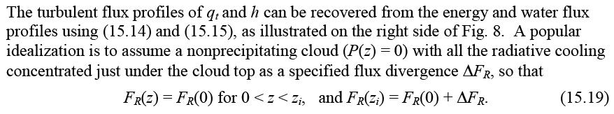
11 Atm S 547 Boundary-Layer Meteorology Bretherton (dq*/dz) da - 4 g kg -1 km -1. Hence, (15.2) simplifies to z b (q* Ms - q tm ) / dq*/dz da (15.6) If the surface air is more subsaturated, z b will be larger. A good approximation is that if the near-surface relative humidity is 80%, the cloud base (= lifted condensation level) will be about 500 m. If the near surface RH is 60%, the cloud base will be 1 km, etc. Above the cloud base, similar linearization gives the liquid water profile q l (z) = q tm - q*(p M (z), T M(z)) dq*/dz ma (z - z b ), (15.7) where (dq*/dz) ma is the rate at which saturation mixing ratio changes with height above cloud base along a moist adiabat. Typically dq*/dz ma 2 g kg -1 km -1 is about half as large as dq*/dz da in a stratocumulus layer. We see that the liquid water content is largest at the cloud top, and that the vertically-integrated cloud liquid water content, or liquid water path, is proportional to the square of the cloud layer depth. An adiabatic subtropical stratocumulus cloud about 300 m thick has a cloud-top liquid water content of 0.6 g kg -1 and a liquid water path of about 100 g m -2. Fig. 8 (left) shows how various profiles behave in a stratocumulus-capped mixed layer. MLM equations Above the boundary layer, we assume known free-tropospheric profiles q t + (z), h + (z). These affect the entrainment flux into the mixed layer: w! q t!(z i ) = "w e #q t,!q t = q + (z i ) " q tm, (15.8a) w! h!(z i ) = "w e #h,!h = h + (z i ) " h tm. (15.8b) Since stratocumulus evolve slowly, we must also consider the mean vertical velocity w (z), which is often idealized as subsidence that increases linearly with height: w (z) = -Dz, (15.9) where D is the horizontal wind divergence, typically s -1 in subtropical stratocumulus regimes. Thus, at a height of 1 km, the mean subsidence rate is around 3-6 mm s -1. This is slow but significant. Another important boundary condition is the sea-surface temperature T s, which determines the surface heat and moisture fluxes. From T s, we calculate the mixing ratio within the seasurface skin layer, q s = q*(p s, T s ) and the sea-surface moist static energy h s = c p T s + Lq s. For simplicity, we will only model the thermodynamic evolution of a SCBL, not its momentum balance, so we will just specify a mixed-layer wind speed V, and we will use bulk aerodynamic formulas with a nondimensional transfer coefficient C T (V) 10-3 to specify the surface fluxes: w! q t!(0) = C T V(q s " q tm ), w! h!(0) = C T V(h s " h tm ). (15.10a) (15.10b) Within the boundary layer, there will be a net upward radiative flux profile F R (z) (including both longwave and shortwave contributions) and a downward water flux profile P(z) due to precipitation. These fluxes must be diagnosed from the mixed layer properties, including the vertical structure of the cloud layer, following the ideas presented in Lecture 2. Here we will just assume we have some algorithm for doing this. We must also have an entrainment closure for specifying the entrainment rate w e, which we ll discuss later. Now we are finally ready to write down the governing equations for the MLM, which express conservation of mass, water, and moist static energy in the mixed layer: 15-6

12 dz i dt = w e + w(z i ), (15.11) dh M dt dq tm dt =! 1 #E " #z, (15.12) =! 1 #W " #z. (15.13) Here, d/dt is the material derivative following the boundary layer air column, which moves with the mean horizontal wind. Furthermore, W(z) = ρ w! q t!(z) " P(z) (15.14) is the upward water flux, composed of a turbulent and precipitation flux, and E(z) = ρ w! h!(z) + F R (z) (15.15) is the upward energy flux, composed of a turbulent and a radiative flux.

13 If we know w e from the entrainment closure, the MLM equations can be solved as in the dry case. Since the left hand sides of ( ) are height-independent, the same must be true of their right hand sides. Hence, the energy and water fluxes must vary linearly with height between the surface and the inversion. Defining a nondimensional height ζ = z/z i : and where W(z) = (1- ζ)w(0) + ζw(z i ), E(z) = (1- ζ)e(0) + ζe(z i ), (15.16a) (15.16b)! "W "z = W (0)! W (z i ) z i, (15.17a)! "E "z = E(0)! E(z i ) z i, (15.17b) W(0) = ρc T V(q s - q tm ) - P(0), W(z i ) = - ρw e Δq t, (15.18a) E(0) = ρc T V(h s - h tm ) + F R (0), E(z i ) = - ρw e Δh + F R (z i ). (15.18b) This completes the specification of the right-hand sides of ( ), allowing the MLM equations to be marched forward in time.

14

15

16 Parcel circuits in a Sc-capped mixed layer Note implied discontinuous increase in liquid water and buoyancy fluxes at cloud base turbulence driven from cloud, unlike dry CBL. Convective velocity w * ~ 1 m s -1 : w 3 * = 2.5 w b dz 0 z i Lecture 15, Slide

17 To mathematically express the buoyancy flux in terms of the fluxes of q t and h that are calculated by the MLM, we must express T v in terms of their perturbations q t and h. For simplicity, we will only derive this for the most important term in T v, which is the temperature perturbation T. We start by noting q t = q v + q l, h c p T + Lq v. Below cloud base in unsaturated air (q l = 0), this gives the desired relationship: T = [h - Lq t ]/c p. (below cloud base) (15.24)

18 Above cloud base, the air is saturated. Using the Clausius-Clapeyron equation, q v = q * = (dq * /dt) T = (γ c p /L) T, where γ = (L/c p ) dq * /dt = 1-3 (larger at higher temperature). Hence and h c p T + Lq v = (1 + γ ) c p T, T = h /[c p (1 + γ )]. (above cloud base) (15.25) It is also physically helpful to write T = [h - Lq t + Lq l ]/c p. Above cloud base, the latent heating due to condensation of more liquid water (q l > 0) is reflected in higher temperature (T > 0).

19 With a bit more algebra, one can generalize these formulas to T v (Randall 1981): T v = [h - µlq t ]/c p. (below cloud base) (15.26a) T v = [βh - εlq t ]/c p. (above cloud base) (15.26b) where: ε = c p T 0 /L 0.12, (15.27) µ =1 δε 0.93, (15.28) β = (1 + γε(1 + δ))/(1 + γ ) (15.29)

20

21 Entrainment Rate Parameterization in Shallow Convecting Layers Consider the TKE budget in the entrainment zone at the top of a clear convective boundary layer capped by a stable interface. In the entrainment zone, transport of TKE into the zone (and possible shear generation of TKE) must balance destruction by entrainment, dissipation, and storage (see TKE budget plot). Dimensional arguments following Tennekes (1973) suggest that for a fully turbulent boundary layer with turbulent velocity scale U and depth z i, transport, dissipation and entrainment will all be O(U 3 /z i ). For a sheardriven boundary layer, the shear production will also be of this order, while the storage term is much smaller if the entrainment zone is strongly stratified.

22 Hence the entrainment buoyancy flux (w θ v) e should scale as (w b ) e = AU 3 /z i, (1) where A is an empirical constant. For a discontinuous inversion with a buoyancy jump θ v, (w θ v) e = w e θ v. (2) By substituting (2) into (1), we obtain w e = AU 3 z i θ v, (3) which can be expressed in terms of a bulk interfacial Richardson number Ri = z i θ v /U 2 as w e U = A z i θ v /U = A 2 Ri. (4)

23

24 From the buoyancy flux profile, we calculate the convective velocity w * as for the DCBL: and then we calculate the entrainment rate as w 3 * = 2.5! B(z)dz, (15.19) 0 z i w e = A w * 3 /(z i Δb), (15.20) where the entrainment efficiency A = 0.2(1 + a 2 E). (15.21) Here E is a dimensionless parameter (see Fig. 10) that describes how much evaporation of cloud liquid water reduces the buoyancy of mixtures of mixed-layer and above-inversion air.

25 Sc MLM entrainment closure Nicholls-Turton (1986) entrainment closure Fit to aircraft and lab obs and dry CBL 3 w e = A w * z i Δb, A = 0.2(1+ a 2E), Δb = g ΔT v T 0 Evaporative enhancement: Less buoyant mixtures easier to entrain. Observational test with SE Pacific Sc diurnal cycle (Caldwell et al. 2005) NT enhancement factor E = Δ m /ΔT v a 2 = A = in typical Sc T v ρ 0 χ * 0.1 Entrained fraction χ 1 2Δ m ΔT v NT: Nicholls and Turton (1986) DL: Lilly (2002) LL: Lewellen&Lewellen (2003) Lecture 15, Slide

26 E ranges from 0 (when no cloud is present) to 0.2 or more (for a thick cloud with very dry overlying air or a weak capping inversion). The empirical constant a 2 is in the range The width of this range reflects the large measurement uncertainties for entrainment rate, and reflects studies by Nicholls and Turton (1986), Stevens et al. (2003) and Caldwell et al. (2005). The term a 2 E reflects evaporative enhancement of entrainment and raises the entrainment efficiency of typical stratocumulus into the range 0.5-2, compared to its dry value of 0.2. Lilly (2002) proposed a related entrainment closure that has some conceptual improvements over Nicholls-Turton, but probably has little practical advantage.

27 A complication with applying (15.20) is that the buoyancy flux, and hence w * 3, depends on w e. However, we can partition w * 3 into a term proportional to entrainment and a nonentrainment term due to other processes such as surface fluxes, radiative cooling, etc.: w * 3 = (w * 3 ) ne + w e dw * 3 When this is substituted into (15.20), we can solve for w e. dw e. (15.22)