A Study on the Relationship between the Air-Sea Density Flux and Isopycnal Meridional Overturning Circulation in a Warming Climate

Transcription

1 University of Miami Scholarly Repository Open Access Theses Electronic Theses and Dissertations A Study on the Relationship between the Air-Sea Density Flux and Isopycnal Meridional Overturning Circulation in a Warming Climate MyeongHee Han University of Miami, mhan@rsmas.miami.edu Follow this and additional works at: Recommended Citation Han, MyeongHee, "A Study on the Relationship between the Air-Sea Density Flux and Isopycnal Meridional Overturning Circulation in a Warming Climate" (211). Open Access Theses This Open access is brought to you for free and open access by the Electronic Theses and Dissertations at Scholarly Repository. It has been accepted for inclusion in Open Access Theses by an authorized administrator of Scholarly Repository. For more information, please contact repository.library@miami.edu.

2 UNIVERSITY OF MIAMI A STUDY ON THE RELATIONSHIP BETWEEN THE AIR-SEA DENSITY FLUX AND ISOPYCNAL MERIDIONAL OVERTURNING CIRCULATION IN A WARMING CLIMATE By MyeongHee Han A THESIS Submitted to the Faculty of the University of Miami in partial fulfillment of the requirements for the degree of Master of Science Coral Gables, Florida May 211

3 211 MyeongHee Han All Rights Reserved

4 UNIVERSITY OF MIAMI A thesis submitted in partial fulfillment of the requirements for the degree of Master of Science A STUDY ON THE RELATIONSHIP BETWEEN THE AIR-SEA DENSITY FLUX AND ISOPYCNAL MERIDIONAL OVERTURNING CIRCULATION IN A WARMING CLIMATE MyeongHee Han Approved: Igor Kamenkovich, Ph.D. Associate Professor of Meteorology and Physical Oceanography Terri A. Scandura, Ph.D. Dean of the Graduate School William E. Johns, Ph.D. Professor of Meteorology and Physical Oceanography Timour Radko, Ph.D. Professor of Physical Oceanography Naval Postgraduate School

5 HAN, MYEONGHEE (M.S., Meteorology and Physical Oceanography) A Study on the Relationship (May 211) between the Air-Sea Density Flux and Isopycnal Meridional Overturning Circulation in a Warming Climate Abstract of a thesis at the University of Miami. Thesis supervised by Professor Igor Kamenkovich. No. of pages in text. (91) The Meridional Overturning Circulation (MOC) plays an important part in the Earth s climate, but the mechanisms that determine MOC response to climate change remain unclear. In particular, the relative importance of the adiabatic and diabatic dynamics in MOC is still under debate. This study aims to explore the relationship between the airsea density flux and isopycnal MOC, and examine the possibility of diagnosing the adiabatic component of MOC from the air-sea density flux. This is done here using the concept of the push-pull mode, which consists of the adiabatic push into the deep ocean in the Northern Hemisphere and pull out of the deep ocean in the Southern Hemisphere. The evolutions of the isopycnal MOC and the push-pull mode are qualitatively similar. The maximum streamfunctions of the push-pull modes and isopycnal MOC both decrease by 3-5 Sv during 1 years, and their decrease is very similar to each other in the deep layers. In particular, the slope of the downward linear trend in the maximum is about -5 Sv per 1 years in both the push-pull modes and isopycanl MOC at the equator. The decrease in actual isopycnal MOC is faster at heavier densities than that at lighter densities. The first EOF mode of eigenvectors of the push-pull mode explains less percentage of variance than in the case of the isopycnal MOC at the equator. The

6 detection of the global changes in MOC from the surface fluxes alone is feasible, if the surface fluxes are measured with sufficient accuracy.

7 Dedicated to my parents and sisters iii

8 Acknowledgements I want to sincerely thank my advisor, Dr. Igor Kamenkovich for helping me with many things for the first 3 years studying in the United States. I also want to thank my other committee members, Dr. William E. Johns and Dr. Timour Radko for advice on my thesis. I also want to thank Dr. Dughong Min, Dr. Sang-Ki Lee, Dr. Arthur Mariano, Dr. Kevin Leaman, and all professors and students who helped me at RSMAS. Especially I want to thank my lovely parents and sisters; this thesis is dedicated to them. iv

9 TABLE OF CONTENTS Page LIST OF FIGURES... LIST OF TABLES... vi xii Chapter 1 INTRODUCTION Motivation and background METHODOLOGY Push-pull mode and isopycnal streamfunction Model output RESULTS Air-sea density flux The Atlantic Ocean Surface push-pull component Full push-pull component Interannual variability in the overturning Interdecadal variability in the overturning The Indo-Pacific Ocean Surface push-pull component Full push-pull component Interannual variability in the overturning Interdecadal variability in the overturning The World Ocean Surface push-pull component Full push-pull component Interannual variability in the overturning Interdecadal variability in the overturning SUMMARY AND CONCLUSIONS REFERENCES... 9 v

10 LIST OF FIGURES Figure Page 1.1 Evolution of the Atlantic meridional overturning circulation (MOC) at 3 N in simulations with the suite of comprehensive coupled climate models from IPCC AR4 (Meehl et al. 27) In a simplified 4 different density (σ i, i =,1,2,3,4) layer ocean, push-pull mode from 3 S to N or to N can be estimated by the air-sea volume flux of the Southern and Northern hemisphere (B s, B n ), the actual isopycnal MOC (V lat ), and cross-isopycnal volume flux (V d ). The push-pull mode starts from 3 S to avoid including the air-sea volume flux ( B s3, B s4 ) in the Antarctic Circumpolar Current (ACC), so it includes B s1 and B s2 only in the Southern Hemisphere Difference between the last five-year and first five-year averaged air-sea density fluxes in the World Ocean. Left panel: GFDL model. Right panel: NCAR model Difference of zonally averaged density flux (red), fresh water part of density flux (green), and heat flux part of density flux (blue) between the last five-year and first five-year means in the World Ocean. Left panel: GFDL model. Right panel: NCAR Potential density differences at the surface between the last five-year and first five-year means in the World Ocean. Left panel: GFDL model. Right panel: NCAR model Sea ice concentration in year 2 and 21 in the World Ocean. Left panel: GFDL model. Right panel: NCAR model The first five-year (dotted line) and last five-year (solid line) means of the surface push-pull mode (3 S to N) with density flux (red), fresh water flux part (green), and heat flux part (blue) in the Atlantic Ocean. Left column: GFDL model. Right column: NCAR model Time series of the SPP a with density flux (first row), fresh water flux part (second row), and heat flux part (third row) in the Atlantic Ocean during 1 years. Stars show the density corresponding to the maximum streamfunction in the same year. Left panel: GFDL model. Right panel: NCAR model The first five-year (dotted line) and last five-year (solid line) mean of the PP a (red), PP a (green), Ψ a, and Ψ a 26N (blue) in the Atlantic Ocean. Top row: pushpull mode and actual isopycnal MOC streamfunction (Equator). Bottom row: vi

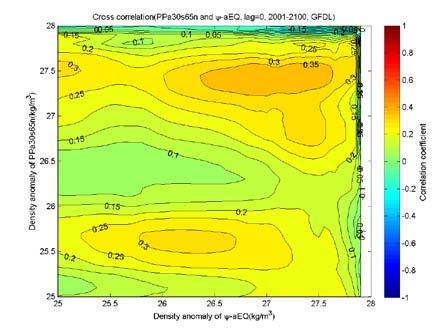
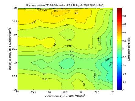
11 push-pull mode and actual isopycnal MOC streamfunction(26.5 N). Left column: GFDL model. Right column: NCAR model Time series of the PP a in the Atlantic Ocean during 1 years. Stars show the density corresponding to the maximum PP a in the same year. Left panel: GFDL model. Right panel: NCAR model Time series of the PP a in the Atlantic Ocean. Stars show the density where PP a reaches maximum in the same year. Left panel: GFDL model. Right panel: NCAR model Time series of the Ψ a in the Atlantic Ocean. Stars show the density at which the streamfunction has a maximum in the same year. Left panel: GFDL model. Right panel: NCAR model Time series of the Ψ a 26.5N in the Atlantic Ocean. Stars show the density at which the streamfunction reaches a maximum in the same year. Left panel: GFDL model. Right panel: NCAR model Time series of the maximum in the PP a, PP a, Ψ a, and Ψ a 26.5N in the Atlantic Ocean. Left panel: GFDL model. Right panel: NCAR model Slope of linear trend of the absolute PP a, PP a, and Ψ a as functions of density in the Atlantic Ocean. Left panel: GFDL model. Right panel: NCAR model Slope of the linear trend of the absolute actual isopycnal MOC as functions of density and latitude (1-degree resolution) in the Atlantic Ocean. Left panel: GFDL model. Right panel: NCAR model Cross correlation between density pairs for the push-pull mode (PP a and PP a ) and actual isopycnal MOC (Ψ a and Ψ a 26.5N ) in the Atlantic Ocean. First panel: PP a andψ a. Second panel: PP a and Ψ a 26.5N. Third panel: PP a and Ψ a. Fourth panel: PP a and Ψ a 26.5N. Left panel: GFDL model. Right panel: NCAR model Maximum cross correlation among all density pairs among PP a, PP a, Ψ a, and Ψ a 26.5N in the Atlantic Ocean, for various values of time lag. Left panel: GFDL model. Right panel: NCAR model. The values of density are reported for maximum correlations. Maximum correlation coefficient is noted by negative lag (green), lag (blue), positive lag (black) Eigenvectors of thepp a, PP a, Ψ a 3S, Ψ a, Ψ a 26.5N, Ψ a N, and Ψ a N as functions of density in the Atlantic Ocean. First mode (red), Second mode (green), Third mode (blue). Left panel: GFDL model. Right panel: NCAR model vii

12 3.18 Power Spectral Density (PSD) of the PP a, PP a, Ψ a 3S, Ψ a, Ψ a 26.5N, Ψ a N, and Ψ a N as functions of frequency(year-1) in the Atlantic Ocean. First mode (red), Second mode (green), Third mode (blue). Left panel: GFDL model. Right panel: NCAR model Cross correlation between density pairs for the low-pass filtered PP a and PP a, Ψ a, and Ψ a 26.5N in the Atlantic Ocean. First panel: PP a and Ψ a. Second panel: PP a and Ψ a 26.5N. Third panel: PP a and Ψ a. Fourth panel: PP a and Ψ a 26.5N. Left panel: GFDL model. Right panel: NCAR model Maximum cross correlation among all density pairs between the low-pass filtered PP a, PP a, Ψ a, and Ψ a 26.5N in the Atlantic Ocean, for various values of time lag. Left panel: GFDL model. Right panel: NCAR model. The values of density are reported for maximum correlations. Maximum correlation coefficient is shown with bracket The first five-year (dotted line) and last five-year (solid line) mean of the surface push-pull mode (3 S to N) with density flux (red), fresh water flux part (green), and heat flux part (blue) in the Indo-Pacific Ocean. Left column: GFDL model. Right column: NCAR model Time series of the SPP ip with density flux (first row), fresh water flux part (second row), and heat flux part (third row) in the Indo-Pacific Ocean during 1 years. Stars show the density corresponding to the maximum streamfunction in the same year. Left panel: GFDL model. Right panel: NCAR model The first five year (21~25 or 2~24, dotted line) and the last five year (296~21 or 295~299, solid line) mean of the PP ip (red), PP ip (green), and Ψ ip (blue) in the Indo-Pacific Ocean. Left panel: GFDL model. Right panel: NCAR model Time series of the PP ip in the Indo-Pacific Ocean. Stars show the density corresponding to the maximum streamfunction in the same year. Left panel: GFDL model. Right panel: NCAR model Time series of the PP ip in the Indo-Pacific Ocean. Stars show the density corresponding to the maximum streamfunction in the same year. Left panel: GFDL model. Right panel: NCAR model Time series of the Ψ ip in the Indo-Pacific Ocean. Left panel: GFDL model. Right panel: NCAR model Time series of the maximum magnitude of the PP ip (red), PP ip (green), and Ψ ip (blue) in the Indo-Pacific Ocean. Left panel: GFDL model. Right panel: NCAR model viii

13 3.28 Slope of the linear trend of the absolute PP ip, PP ip, and Ψ ip as functions of density in the Indo-Pacific Ocean. Left panel: GFDL model. Right panel: NCAR model Slope of the linear trend of the absolute actual isopycnal MOC as functions of density and latitude (1-degree resolution) in the Indo-Pacific Ocean. Left panel: GFDL model. Right panel: NCAR model Cross correlation between two density of the PP ip, PP ip, and Ψ ip in the Indo- Pacific Ocean. Upper panel: PP ip and Ψ ip. Lower panel: PP ip and Ψ ip. Left panel: GFDL model. Right panel: NCAR model Maximum cross correlation among all density pairs for the PP ip, PP ip, and Ψ ip in the Indo-Pacific Ocean for various values of time lag. Left panel: GFDL model. Right panel: NCAR model. The values of density are reported for maximum correlations. Maximum correlation coefficient is shown with bracket Eigenvectors of the PP ip, PP ip, Ψ ip 3S, Ψ ip, Ψ ip N, and Ψ ip N as functions of density in the Indo-Pacific Ocean. First mode (red), Second mode (green), Third mode (blue). Left panel: GFDL model. Right panel: NCAR model Power Spectral Density (PSD) of the PP ip, PP ip, Ψ ip 3S, Ψ ip, Ψ ip N, and Ψ ip N as functions of frequency(year-1) in the Indo-Pacific Ocean. First mode (red), Second mode (green), Third mode (blue). Left panel: GFDL model. Right panel: NCAR model Cross correlation between two density of low-pass filtered PP ip, PP ip, and Ψ ip in the Indo-Pacific Ocean. Upper panel: push-pull mode (from 3 S to N) and actual isopycnal MOC ( ). Lower panel: push-pull mode (from 3 S to N) and actual isopycnal MOC ( ). Left panel: GFDL model. Right panel: NCAR model Maximum cross correlation among all density pairs between two density for the low-pass filtered PP ip, PP ip, and Ψ ip in the Indo-Pacific Ocean for various values of time lag. Left panel: GFDL model. Right panel: NCAR model. The values of density are reported for maximum correlations. Maximum correlation coefficient is shown with bracket at zero time lag The first five-year (dotted line) and last five-year (solid line) mean of the SPP w with density flux (red), fresh water flux part (green), and heat flux part (blue) in the World Ocean. Left column: GFDL model. Right column: NCAR model ix

14 3.37 Time series of the SPP w with density flux (first row), fresh water flux part (second row), and heat flux part (third row) in the World Ocean during 1 years. Stars * show the maximum streamfunction. Left panel: GFDL model. Right panel: NCAR model The first five-year (dotted line) and last five-year (solid line) mean of the PP w (red), PP w (green), and Ψ w (blue) in the World Ocean. Left panel: GFDL model. Right panel: NCAR model. The first five year mean (21~25 or 2~24, dotted line) and the last five year mean (296~21 or 295~299, solid line) Time series of the PP w in the World Ocean during 1 years. Stars show the density corresponding to the maximum streamfunction. Left panel: GFDL model. Right panel: NCAR model Time series of the PP w in the World Ocean. Stars show the density corresponding to the maximum streamfunction in the same year. Left panel: GFDL model. Right panel: NCAR model Time series of the Ψ w in the World Ocean. Stars show the density corresponding to the maximum streamfunction in the same year. Left panel: GFDL model. Right panel: NCAR model Time series of the maximum PP w, PP w and Ψ w in the World Ocean. Left panel: GFDL model. Right panel: NCAR model Slope of the linear trend of the absolute PP w, PP w, and Ψ w as functions of density in the World Ocean. Left panel: GFDL model. Right panel: NCAR model Slopes of the linear trend in the absolute actual isopycnal MOC (3 S, 2 S, 1 S,, 1 N, 2 N, 3 N, 4 N, N, 6 N, N) as functions of density and latitude in the World Ocean. Left panel: GFDL model. Right panel: NCAR model Cross correlation between two densities of the PP w, PP w, and Ψ w in the World Ocean. First panel: push-pull mode (from 3 S to N) and isopycnal actual MOC ( ). Second panel: push-pull mode (from 3 S to N) and isopycnal actual MOC ( ). Left panel: GFDL model. Right panel: NCAR model Maximum cross correlation among all density pairs for the PP w, PP w, and Ψ w in the World Ocean, for various values of time lag. Left panel: GFDL model. Right panel: NCAR model. Maximum correlation coefficient is shown with bracket x

15 3.47 Eigenvectors of the PP w, PP w, Ψ w 3S, Ψ w, Ψ w N, and Ψ w N as functions of density in the World Ocean. First mode (red), Second mode (green), Third mode (blue). Left panel: GFDL model. Right panel: NCAR Power Spectral Density (PSD) of the PP w, PP w, Ψ w 3S, Ψ w, Ψ w N, and Ψ w N as functions of frequency(year-1) in the World Ocean. First mode (red), Second mode (green), Third mode (blue). Left panel: GFDL model. Right panel: NCAR model Cross correlation between two densities of the interdecadal anomalies in the PP w, PP w, and Ψ w in the World Ocean. First panel: PP w and Ψ w. Second panel: PP w and Ψ w. Left panel: GFDL model. Right panel: NCAR model Maximum cross correlation among all density pairs between two densities of the interdecadal anomalies in the PP w, PP w, and Ψ w in the World Ocean, for various values of time lag. Left panel: GFDL model. Right panel: NCAR model. Maximum correlation coefficient is shown with bracket xi

16 LIST OF TABLES Table Page 3.1 Changes of SPP a with density flux, fresh water flux part, and heat flux part in the Atlantic Ocean during 1 years. Red shows the maximum streamfunction in the same year Changes of PP a, PP a, Ψ a, and Ψ a 26N in the Atlantic Ocean between the first five-year mean and last five-year mean. Red shows the maximum streamfunction in the same year First five-year and last five-year mean streamfunctions of PP a, PP a, Ψ a, and Ψ a 26N as functions of density in the Atlantic Ocean Changes of the PP a in the Atlantic Ocean during 1 years. Red shows the maximum streamfunction in the same year Changes of PP a in the Atlantic Ocean during 1 years. Red shows the maximum streamfunction in the same year Changes of the Ψ a in the Atlantic Ocean during 1 years. Red shows the maximum streamfunction in the same year Changes of Ψ a 26.5N in the Atlantic Ocean during 1 years. Red shows the maximum streamfunction in the same year Changes of the SPP ip with density flux, fresh water flux part, and heat flux part in the Indo-Pacific Ocean during 1 years. Red shows the maximum streamfunction in the same year Changes in the full PP ip, PP ip, and Ψ ip in the Indo-Pacific Ocean between the first five-year mean and last five-year mean. Red shows the maximum streamfunction in the same year Changes of PP ip in the Indo-Pacific Ocean during 1 years. Red shows the maximum streamfunction in the same year Changes in the PP ip in the Indo-Pacific Ocean during 1 years. Red shows the maximum streamfunction in the same year Changes of in the Ψ ip in the Indo-Pacific Ocean during 1 years. Red shows the maximum streamfunction in the same year xii

17 3.13 Changes of the SPP w with density flux, fresh water flux part, and heat flux part in the World Ocean during 1 years. Red shows the maximum streamfunction in the same year Changes of the PP w (red), PP w (green), and Ψ w (blue) in the World Ocean between the first five-year mean and last five-year mean. Red shows the maximum streamfunction in the same year First five-year mean and last five-year mean streamfunction of the PP w (red), PP w (green), and Ψ w (blue) as functions of density in the World Ocean Changes of the PP w in the World Ocean during 1 years. Red shows the maximum streamfunction in the same year Changes of the PP w in the World Ocean during 1 years. Red shows the maximum streamfunction in the same year Changes of the Ψ w in the World Ocean during 1 years. Red shows the maximum streamfunction in the same year xiii

18 Chapter 1 Introduction 1.1 Motivation and background The Climate of the Earth is strongly affected by the ocean circulation, which carries massive amount of heat from the tropics to the poles and from the pole to the pole in the ocean (Talley et al. 23; Boccaletti et al. 25). In particular, the Meridional Overturning Circulation (MOC), zonally integrated meridional flow in the ocean (Wunsch 22), plays an important part in the Earth s climate (Stouffer et al. 26) and understanding its dynamics is crucial as the sea surface temperature increases in the 21st century (Clark et al. 22). However, the mechanisms of MOC and the response to the climate change remain largely unclear. According to the Intergovernmental Panel on Climate Change (IPCC) future climate projections, the Atlantic MOC will slow down in the 21 st century, but the magnitudes of the reduction varies between the models (Fig.1.1; Meehl et al. 27). This uncertainty outlines the importance of the studies of mechanisms of MOC dynamics and its response to changes in atmospheric conditions. Because there is temperature difference in the ocean, the thermal movement occurs between low latitudes and high latitudes, and between surface and subsurface. At the surface layer and the deep water, Walin (1982) found that the thermal circulation between the tropics and the pole is related to the thermal forcing at the sea surface and the continuity of volume and heat can be used to calculate it. The study calculated the surface forcing component of the thermohaline circulation using heat and freshwater flux in several regions of the North Atlantic. Marsh (2) found that the variability of 1

19 2 surface forcing is related to the North Atlantic Oscillation (NAO) and the Arctic Oscillation (AO). Furthermore, Grist et al. (29) used the surface thermohaline forcing to examine the variability in the Atlantic MOC, using model outputs of IPCC and linked it to the overturning circulation. Figure 1.1 Evolution of the Atlantic meridional overturning circulation (MOC) at 3 N in simulations with the suite of comprehensive coupled climate models from IPCC AR4 (Meehl et al. 27). MOC is driven by adiabatic and diabatic processes. Below the mixed layer, we can identify two main mechanisms driving MOC. In one mode, MOC is controlled by diabatic mixing, resulting in cross-isopycnal motions, such as upwelling. In the second, semi-adiabatic mode, the water is moving along isopycnals, forced by mass exchanges with the mixed layer above; the cross-isopycnal fluxes can be neglected (Radko 27). Below the mixed layer, such an adiabatic component can be diagnosed from the surface density fluxes. This is the push-pull mode whose lower branch describes the isopycnal pull in the Southern Ocean and the isopycnal push from the north. The adiabatic component in the mixed layer can, therefore, be matched to that in the deep

20 3 ocean and the variability of isopycnal subduction in the mixed layer can be related to that in the actual isopycnal MOC. The MOC can be described well by the adiabatic push-pull component of MOC if it is dominant over the diabatic component (Radko et al. 28). The push-pull MOC represents the component of MOC directly forced by the surface buoyancy fluxes, and can be computed using surface density and air-sea density flux diagnosed from surface heat and fresh water fluxes. Using the output of a numerical model, Radko et al. (28) concluded that approximately two-thirds of MOC can be driven by adabatic processes; the study suggested that the share of the adiabatic component is likely to be even bigger if the contribution of the diapycnal mixing is reduced. The main objectives of this study are to understand how and why the adiabatic MOC changes, to explore a possibility of predicting the actual isopycnal MOC using the push-pull mode, and to compare the variations in the actual isopycnal MOC with those in the push-pull mode. Because these are poorly observed fields, and this study looks into future changes in MOC, the MOC components will be diagnosed using two climatemodel simulations of the 21 st century and the effects of global warming on these components will be studied in the Atlantic, the Indo-Pacific, and the World Ocean.

21 Chapter 2 Methodology 2.1 Push-pull mode and isopycnal stramfunction The methodology for calculating the semi-adiabatic mode of circulation, the push-pull mode, described in this section is adapted from Radko et al. (28); only a brief description is given here. Air-sea density flux (B ) into the ocean can be calculated using surface temperature, salinity, and heat and fresh water fluxes and defined as below (Schmitt et al. 1989). B = αh (E P R)S + βρ C p 1 S α = ρ T β = ρ S E = Q lat L B : air-sea density flux in to the ocean (kg/m 2 s) α : thermal expansion coefficient (positive) β : haline contraction coefficient (positive) C p : specific heat capacity of seawater E, P : rates of evaporation and precipitation H : heat flux into the ocean (Q sw +Q lw +Q lat +Q sen ) L : latent heat of evaporation ( J kg -1 ) ρ : density Q lat : surface Latent Heat Flux R : runoff S : salinity T : temperature All calculations are carried in the density space, using potential density referenced to the surface. Maximum potential densities in this study are kg/m 3 in the 4

22 5 GFDL model and 128. kg/m 3 in the NCAR model, and for convenience, we use the potential density anomaly (2.5). The range of potential density anomalies ( density hereafter) used in this study is between 22. kg/m 3 and 28. kg/m 3. σ = ρ pot 1 [kg/m 3 ] 2.5 σ ρ pot : potential density anomaly : potential density The isopycnal streamfunction is calculated using the vertical integration of the meridional volume flux is as follows. v V σ x e Ψ(σ) = v(x, σ )dxdσ = V(σ )dσ [m 3 s] 2.6 σ max x w σ max : meridional velocity : meridional volume flux σ Because the volume is conserved, the convergence of air-sea volume flux (B), the cross-isopycnal volume flux, and the along-isopycnal volume flux are equal to zero. It is shown that the diabatic eddies of the air-sea density flux is smaller than other terms and can generally be neglected in the mixed layer, in most of the domain (Radko, 27). Therefore, the volume flux of fluid subducted on the bottom of mixed layer is the sum of the difference of the diapycnal advective volume flux and the air-sea volume flux. If the divergence of the diapycnal advective volume fluxes is small enough to be negligible, the subducted volume flux on the bottom of mixed layer is equal to the air-sea volume flux. Under the assumptions, the actual isopycnal volume flux in the subsurface ocean can be diagnosed from the air-sea density flux (B ). This is referred to as the push-pull mode (Fig. 2.1).

23 6 The regions south of approximately 3 S and north of approximately N present a challenge for these estimates for several reasons. Firstly, these regions are characterized by a deep mixed layer, for which the diabatic processes, not accounted for by the push-pull mode approach, are important. Secondly, the lack of meridional boundaries in the southern Atlantic Ocean significantly complicates the calculation of the push-pull mode (Radko et al. 28). Lastly, the presence of sea ice in high latitudes (Fig. 3.4) further complicates the analysis, since the ice-ocean heat/fresh water fluxes for these simulations are not available to us from data portal. To address these problems at high latitudes, the push-pull mode is calculated from the sea surface flux and density not over all latitudes, but for the region between 3 S and N (or N) in the Atlantic. The isopycnal volume fluxes into this domain from high latitudes are included into the analysis, as explained below. Fig. 2.1 illustrates the concept on the example of four isopycnal layers. Assume that the air-sea volume flux (B) into the ocean, the cross-isopycnal volume flux (V d ), and the along-isopycnal volume flux (V lat ) are known in four density layers (σ i, i=, 1, 2, 3, 4). The push-pull mode from 3 S to N can then be determined by following procedure: In the Southern Hemisphere (from 3 S to the Equator), the convergence of volume flux is equal to zero in all layers: B s (σ 1 ) + V ds (σ 1 ) V ds (σ ) V eq (σ 1 ) = 2.7 B s (σ 2 ) + V ds (σ 2 ) V ds (σ 1 ) V eq (σ 2 ) = 2.8 V 3s (σ 3 ) + V ds (σ 3 ) V ds (σ 2 ) V eq (σ 3 ) = 2.9 V 3s (σ 4 ) + V ds (σ 4 ) V ds (σ 3 ) V eq (σ 4 ) = 2.1

24 7 Figure 2.1 In a simplified 4 different density (σ i, i =, 1, 2, 3, 4) layer ocean, push-pull mode from 3 S to N or to N can be estimated by the air-sea volume flux of the Southern and Northern hemisphere (B s, B n ), the actual isopycnal MOC (V lat ), and cross-isopycnal volume flux (V d ). The push-pull mode starts from 3 S to avoid including the air-sea volume flux (B s3, B s4 ) in the Antarctic Circumpolar Current (ACC), so it includes B s1 and B s2 only in the Southern Hemisphere. If (2.7), (2.8), (2.9), and (2.1) are added, the result is as below. B s (σ 1 ) + B s (σ 2 ) + V 3s (σ 3 ) + V 3s (σ 4 ) V eq (σ 1 ) V eq (σ 2 ) V eq (σ 3 ) V eq (σ 4 ) + V ds (σ 4 ) V ds (σ ) = 2.11 The air-sea volume fluxes like B s (σ 3 ) and B s (σ 4 ) in ACC are not included. Similar to the Southern Hemisphere, we can write the following expressions in the Northern Hemisphere (from the Equator to N). B n (σ 1 ) + V eq (σ 1 ) + V dn (σ 1 ) V dn (σ ) = 2.12 B n (σ 2 ) + V eq (σ 2 ) + V dn (σ 2 ) V dn (σ 1 ) = 2.13 B n (σ 3 ) + V eq (σ 3 ) + V dn (σ 3 ) V dn (σ 2 ) = 2.14 V eq (σ 4 ) + V dn (σ 4 ) V dn (σ 3 ) V n (σ 4 ) = 2.15 If (2.12), (2.13), (2.14), and (2.15) are added, the result is as below.

25 8 B n (σ 1 ) + B n (σ 2 ) + B n (σ 3 ) + V eq (σ 1 ) + V eq (σ 2 ) + V eq (σ 3 ) + V eq (σ 4 ) V n (σ 4 ) + V dn (σ 4 ) V dn (σ ) = 2.16 If (2.11) is subtracted from (2.16), the result is as below. V eq (σ 1 ) + V eq (σ 2 ) + V eq (σ 3 ) + V eq (σ 4 ) = 1 2 {B s(σ 1 ) + B s (σ 2 ) B n (σ 1 ) B n (σ 2 ) B n (σ 3 )} {V 3s(σ 3 ) + V 3s (σ 4 ) + V n (σ 4 )} {V dn(σ ) V ds (σ ) + V ds (σ 4 ) V dn (σ 4 )} 2.17 If the contribution of the cross-isopycnal volume flux ( V dn (σ ) V ds (σ ) + V ds (σ 4 ) V dn (σ 4 )) is negligible, which can be true if the distribution of diapycnal fluxes is nearly symmetric around the Equator, (2.17) can be rewritten as the push-pull mode from 3 S to N (PP (σ)) below: PP (σ) = 1 2 {B s(σ) B n (σ)} {V 3s(σ) + V n (σ)} 2.18 The actual isopycnal MOC at the Equator (V eq (σ)) can then be expected to be close to the push-pull mode (PP (σ)) which is a combination of the air-sea volume flux (B s (σ) B n (σ)) and the actual isopycnal MOC at 3 S and N (V 3s (σ) + V n (σ)). The push-pull mode from 3 S to N (PP (σ)) can be written similarly: PP (σ) = 1 2 {B s(σ) B n (σ)} {V 3s(σ) + V n (σ)} 2.19 A number of factors can explain the difference between the push-pull mode and the actual isopycnal MOC at the Equator. Most importantly, finite cross-isopycnal volume

26 9 flux will explain the largest part of the difference. Note also that this technique formally assumes a steady state with unchanging isopycnal position. In this study, we assume that changes in the stratification are sufficiently slow; but changes in the volume of each isopycnal layer can, nevertheless, introduce additional biases. 2.2 Model output Two global-change simulations carried for the Intergovernmental Panel on Climate Change (IPCC) 4th Assessment Report (AR4) are analyzed in this study: one with the GFDL (Geophysical Fluid Dynamics Laboratory) and one with NCAR (National Center for Atmospheric Research) climate models. The scenario of output data is SRES (special Report on Emissions Scenarios) A2, which assumes that the global population will be increasing continuously and the regional economic growth will be achieved regionally. This scenario typically implies the strongest greenhouse forcing for the future (DDC 21). In the case of the GFDL model, version CM2.1 was used. To remove the spherical coordinate singularity of the Arctic Ocean, bipolar grid with singularities over Siberia and Canada was used in the Arctic north of N, so the grid is tripolar including the pole in the Antarctic. Note that our calculations are based on the fields south of this latitude. The horizontal resolutions are 1 degree longitudinal and 1 degree latitudinal with enhanced tropical latitudinal (3 S to 3 N) resolution (1/3 degree). The total size of the horizontal grid is 36 in the zonal and 2 in the meridional (81 S to 9 N) directions. The vertical grid involves 22 evenly spaced cells between the surface and

27 1 22m and 28 cells from 22m to 5m, so the total number of vertical cells is. Partial cells are used at the bottom (Griffies et al., 25). In the case of the NCAR model, the Community Climate System Model (CCSM) version 3. was used. The bipolar grid was used. The horizontal resolution is somewhat higher than in the GFDL counterpart. The longitudinal resolution is degree and the latitudinal resolution is about.5342 degree with enhanced tropical latitudinal resolution (.2671 degree). The total horizontal grids are 32 zonal and 395 meridional (79 S to 9 N) points. There are 4 vertical cells with thicknesses increasing from the surface to 5m (Smith et al., 24).

28 Chapter 3 Results 3.1 Air-sea density flux The air-sea density flux and sea surface density both change during years 2-21, with particularly significant changes in the North Atlantic. The air-sea density flux into the ocean is calculated here using the fresh water and heat fluxes (2.1). The differences in the resulting density flux between the last five-year and first five-year means are shown in Fig. 3.1 (two-dimensional) and Fig. 3.2 (zonally averaged). During the 1 years of simulations, there is an anomalous density flux into the ocean around South Africa, southeastern Australia, and northeastern United States of America and out of the ocean near the south of Greenland (Fig. 3.1). The zonally averaged density flux differences around 6 S and 6 N are negative (Fig. 3.2). The density differences between the last five-year and first five-year means (Fig. 3.3) exhibit the decreases of density in the Indian Ocean and the western tropics in the Pacific Ocean. These changes in the sea surface density and density fluxes lead to significant changes in MOC in the Atlantic basin and globally. In the following analysis, these effects will be studied using a concept of the push-pull mode, which is an estimate of the component of the MOC directly forced by the surface density input. 11

29 12 Figure 3.1 Difference between the last five-year and first five-year averaged air-sea density fluxes in the World Ocean. Left panel: GFDL model. Right panel: NCAR model. Figure 3.2 Difference of zonally averaged density flux (red), fresh water part of density flux (green), and heat flux part of density flux (blue) between the last five-year and first five-year means in the World Ocean. Left panel: GFDL model. Right panel: NCAR model. Figure 3.3 Potential density differences at the surface between the last five-year and first five-year means in the World Ocean. Left panel: GFDL model. Right panel: NCAR model.

30 The Atlantic Ocean As explained in Section 2, two choices for the northern boundary of the computational domain, N and N, are considered. The first domain, 3 S~ N, is almost ice free, whereas the second 3 S~ N includes significant amounts of sea ice in the Northern Hemisphere (Fig. 3.4), which introduces a challenge for this analysis. To examine the importance of the ice for the push-pull mode in the second domain, we compare the push-pull mode calculated from density fluxes with and without fluxes over ice-covered regions. In the first setting, for example, if the sea ice concentration is 1 % in a given grid cell, only 9 % of the surface density flux is used in (2.1). In the second setting, the density fluxes over the ice-covered regions are set to zero in (2.1). In the third setting, the density fluxes over the ice are assumed to be equal to the fluxes below the ice. The differences among the results obtained using these three methods are less than.1 %. We, therefore, conclude that the surface fluxes over ice-covered regions have a secondary importance. In the rest of the discussion, the push-pull mode are calculated from 3 S to N or from 3 S to N without considering the sea ice concentration as in the third setting. Figure 3.4 Sea ice concentration in year 2 and 21 in the World Ocean. Left panel: GFDL model. Right panel: NCAR model.

31 Surface push-pull component To determine the relative importance of heat and fresh water component in (2.1), the push-pull mode is next calculated for the full density flux (SPP D a ), and for fresh F water flux and heat flux components separately (SPP a and SPP H a ). In order to make the analysis more straightforward, the actual isopycnal MOC stramfunction is not added and the resulting function will be referred to as the surface push-pull mode. The first five-year and last five-year means of the surface push-pull mode are shown in Fig. 3.5 as functions of density. The surface push-pull mode using density flux (SPP D a ) and the surface push-pull mode using heat flux part (SPP H a ) are very close to each other in all density layers, especially for the GFDL model, and the fresh water (SPP F a ) contribution is not significant. We conclude that the surface push-pull mode is dominated by the contribution from the heat flux part rather than the fresh water flux. In D particular, there is a significant decrease in the SPP a at the densities heavier than 27. kg/m 3 during 1 years, which will influence to the reduction of the total pushpull mode. The maximum streamfunction of SPP a changes from 8.4 Sv (27. kg/ D m 3, 21~25) to 6.35 Sv (27.3 kg/m 3, 296~21) in the GFDL model and from 6.64 Sv (27.55 kg/m 3, 2~24) to 2.5 Sv (27.4 kg/m 3, 295~299) in the NCAR model among the density heavier than 27. kg/m 3. The maximum streamfunction of H SPP a changes from 9.7 Sv (27.55 kg/m 3, 21~25) to 7.6 Sv (27.25 kg/m 3, 296~21) in the GFDL model and from 6.98 Sv (27. kg/m 3, 2~24) to 2.57 Sv (27.4 kg/m 3, 295~299) in the NCAR model among the density heavier than 27. kg/m 3. The significant differences between the surface push-pull mode and the actual

32 15 isopycnal MOC at heavier density are explained by the rather limited surface are of heavy density in the 3 S- N region. Figure 3.5 The first five-year (dotted line) and last five-year (solid line) means of the surface pushpull mode (3 S to N) with density flux (red), fresh water flux part (green), and heat flux part (blue) in the Atlantic Ocean. Left column: GFDL model. Right column: NCAR model. The maximum in the SPP a decreases its magnitude and shifts to lighter densities over the course of 1 years in Fig There are decreases of 17% (GFDL) and 12% D (NCAR) of maximum SPP a during 1 years, and the density corresponding to a maximum SPP a (σ Ψmax ) shifts to lighter densities: from 27. to kg/m 3 in the GFDL model and from to kg/m 3 in the NCAR model during 1 years. In the maximum of the SPP F a, there is an increase of 4% (GFDL) and a decrease of 2% (NCAR) during 1 years. Corresponding σ Ψmax shifts to lighter densities: from 26.1 to 23.3 kg/m 3 in the GFDL model and from to 24.9 kg/m 3 in the NCAR model during 1 years. In the maximum of the SPP H a, there are decreases of 22% (GFDL) and 14% (NCAR) of maximum during 1 years, and σ Ψmax shifts to lighter densities: from 27. to 26.8 kg/m 3 in the GFDL model and from 27. to kg/m 3 in the NCAR model during 1 years (Table 3.1).

33 16 Table 3.1 Changes of SPP a with density flux, fresh water flux part, and heat flux part in the Atlantic Ocean during 1 years. Red shows the maximum streamfunction in the same year. Model GFDL NCAR Surface push-pull mode with Density (kg/m 3 ) Streamfunction (First year, Sv) Streamfunction (Last year, Sv) Density flux Fresh water flux Heat flux Density flux Fresh water flux Heat flux

34 17 Figure 3.6 Time series of the SPP a with density flux (first row), fresh water flux part (second row), and heat flux part (third row) in the Atlantic Ocean during 1 years. Stars show the density corresponding to the maximum streamfunction in the same year. Left panel: GFDL model. Right panel: NCAR model Full push-pull component Using the air-sea density flux, the full push-pull mode was calculated from SPP a and the actual isopycnal MOC at 3 S, N, and N. If the diapycnal component of MOC is small, the push-pull mode and the actual isopycnal MOC are expected to be nearly identical (Radko et al. 28). Since the diapycnal component in the real ocean and in these simulations is significant, the isopycnal MOC and the push-pull mode are different. Radko et al. (28) argued that this difference can be expected to be the smallest at the Equator, but it is highly dependent on the distribution of the diapycnal mixing in a model. In what follows, we will compare the push-pull mode to the actual isopycnal MOC at two locations: at the Equator (Ψ a ) and at 26.5 N (Ψ 26.5N a ), the latitude of the RAPID-MOCHA array. The first five-year and last five-year mean streamfunctions of push-pull mode (from 3 S to N: PP a and 3 S to N: PP a ) and actual isopycnal MOC are shown in Fig. 3.7, as functions of density. The push-pull mode and the actual isopycnal MOC both weaken in response to the change in buoyancy forcing in the model, and the degree of weakening is similar

35 18 between the two measures of AMOC (Fig. 3.7). The magnitude of this weakening is bigger in the GFDL model than in the NCAR model; there is a noticeable relative maximum around 26. kg/m 3 in the NCAR. There have been decreases of 4.2 Sv (Ψ a ), 5.1 Sv (PP a ), 5.4 Sv (PP a ), 7.3 Sv (Ψ 26.5N a ) in the GFDL model and 2.4 Sv (PP a ), 3.9 Sv (Ψ a ), 4. Sv (PP a ), 5.7 Sv (Ψ 26.5N a ) in the NCAR model between the last five-year and first five-year mean maximum streamfunctions (Table 3.2). The push-pull mode and the actual isopycnal MOC are very close to each other in the heavier density layers, especially for the GFDL model, although some differences are clearly observed. The push-pull mode is the combination of the air-sea density flux and the actual isopycnal MOC at 3 S and N or N, so the changes of the pushpull mode and the actual isopycnal MOC at the Equator and 26.5 N during 1 years can be different especially if the diapycnal component is important. In the GFDL, PP a is 12 ± 8% (mean ± standard deviation, first five-year mean) and 93 ± 1% (last fiveyear mean) of Ψ a at deep layers heavier than kg/m 3. PP a is 113 ± 4% (first fiveyear mean) and 9 ± 5% (last five-year mean) of Ψ a at the density layers heavier than kg/m 3. In the NCAR, PP a is 92 ± 8% (mean ± standard deviation, first five-year mean) and 94 ± 4% (last five-year mean) of Ψ a at deep layers heavier than kg/m 3. And PP a is 64 ± 12% (first five-year mean) and 7 ± 5% (last five-year mean) of Ψ a at the density layers heavier than kg/m 3 (Table 3.3); Between N and N, the surface region with heavier density is smaller in the NCAR than in the GFDL. In the case of the GFDL model, the streamfunctions of PP a and Ψ a look very similar at the densities heavier than 27. kg/m 3 during 21~25 and 296~21. In the case of NCAR model, PP a and Ψ a are similar at the densities heavier than 27.8 kg/m 3 during

36 N 2~24 and 295~299. PP a and Ψ a look alike at the densities heavier than 27. kg/m 3 only in the beginning of the simulation, during years In the GFDL model, the difference between PP a and Ψ a during the same years is less than 1 Sv at the densities heavier than 26.8 kg/m 3 during 21~25 and between kg/m 3 and kg/m 3 during 296~21 and less than 2 Sv at the densities heavier than 26.4 kg/m 3 during 21~25 and between kg/m 3 and kg/m 3 during 296~21. In the NCAR model, the difference between PP a and Ψ a during the same years is less than 2 Sv at the densities heavier than 27.6 kg/m 3 during 2~24 and at the densities heavier than 27.3 kg/m 3 during 295~299. Figure 3.7 The first five-year (dotted line) and last five-year (solid line) mean of the PP a (red), PP a (green), Ψ a, and Ψ a 26N (blue) in the Atlantic Ocean. Top row: push-pull mode and actual isopycnal MOC streamfunction (Equator). Bottom row: push-pull mode and actual isopycnal MOC streamfunction(26.5 N). Left column: GFDL model. Right column: NCAR model.

37 2 Table 3.2 Changes of PP a, PP a, Ψ a, and Ψ a 26N in the Atlantic Ocean between the first five-year mean and last five-year mean. Red shows the maximum streamfunction in the same year. Model Streamfunction Density (kg/m 3 ) GFDL NCAR Mean streamfunction (First 5 years, Sv) Mean streamfunction (Last 5 years, Sv) PP a PP a Ψ a N Ψ a PP a PP a Ψ a N Ψ a Table 3.3 First five-year and last five-year mean streamfunctions of PP a, PP a, Ψ a, and Ψ a 26N as functions of density in the Atlantic Ocean. Density First five-year (21~25) mean (Sv) Last five-year (296~21) mean (Sv) Model σ < PP a PP a Ψ a Ψ a 26.5N PP a PP a Ψ a Ψ a 26.5N GFDL

38 21 Density First five-year (2~24) mean (Sv) Last five-year (295~299) mean (Sv) Model σ < PP a PP a Ψ a 26.5N Ψ a PP a PP a Ψ a 26.5N Ψ a NCAR Each characteristic of MOC is now discussed individually. The maximum in the PP a decreases its magnitude and shifts to lighter density for the course of 1 years; see the push-pull mode as functions of density and time in the Atlantic Ocean in Fig Over the course of 1 years, there are decreases of 28% in the maximum PP a, from Sv at 27.8 kg/m 3 to Sv at kg/m 3, in the GFDL model and of 23%, from Sv at kg/m 3 to 11.9 Sv at 27. kg/m 3, in the NCAR model. At the same time, σ Ψmax shifts to lighter densities: from 27.8 to kg/m 3 in the GFDL model and from to 27. kg/m 3 in the NCAR model (Table 3.4), but there are more variations of σ Ψmax during the latter years (Fig. 3.8). The change in the

39 22 streamfunction at the same density is bigger than that in the absolute maximum. For example, PP a decreases from to 6.91 Sv at 27.8 kg/m 3. Table 3.4 Changes of the PP a in the Atlantic Ocean during 1 years. Red shows the maximum streamfunction in the same year. Model Density (kg/m 3 ) Streamfunction (First year, Sv) Streamfunction (Last year, Sv) GFDL NCAR Figure 3.8 Time series of the PP a in the Atlantic Ocean during 1 years. Stars show the density corresponding to the maximum PP a in the same year. Left panel: GFDL model. Right panel: NCAR model. The changes in the PP a (Fig. 3.9) in the Atlantic Ocean are very similar to those in PP a (Fig. 3.8). There are decreases of 28% in the maximum PP a (from 18.1 Sv at 27. kg/m 3 to 12.9 Sv at 27.2 kg/m 3 ) in the GFDL model and of 47% (from Sv at 27. kg/m 3 to 7.91 Sv at 27. kg/m 3 ) in the NCAR model during 1 years. Simultaneously, σ Ψmax shifts from 27. to 27.2 kg/m 3 in the GFDL model and from 27. to 27. kg/m 3 in the NCAR model (Table 3.5), but there are more variations of σ Ψmax during 1 years (Fig. 3.9). At the fixed isopycnals, changes are larger than those in the maximum. For example, the PP a decreases from 18.1 to 1.63 Sv at 27. kg/m 3 in the Atlantic in the GFDL model.

40 23 It is also noteworthy that the actual isopycnal MOC at N makes a very small contribution to the push-pull mode even at the deepest density levels in both models. This is mainly due to the fact that most of the deep water formation in these models takes place south of this latitude. Additionally the cross-sectional area at N is much smaller than that at 3 S, and much of the water which is heavier than 28. kg/m 3 do not make a significant contribution to MOC because there is no water heavier than 28. kg/m 3 at the Equator in both models. Table 3.5 Changes of the PP a in the Atlantic Ocean during 1 years. Red shows the maximum streamfunction in the same year. Model Density (kg/m 3 ) Streamfunction (First year, Sv) Streamfunction (Last year, Sv) GFDL NCAR Figure 3.9 Time series of the PP a in the Atlantic Ocean. Stars show the density where PP a reaches maximum in the same year. Left panel: GFDL model. Right panel: NCAR model. Changes in the actual isopycnal MOC at the Equator are consistent with those in the push-pull mode. Similar to the push-pull mode, the maximum Ψ a decreases its magnitude and shifts to lighter density over the course of 1 years (Fig. 3.1). In particular, maximum Ψ a decreases by 26% (from 18.1 Sv at kg/m 3 to Sv at

41 kg/m 3 ) in the GFDL model and by 25% (from 18.4 Sv at 27. kg/m 3 to Sv at kg/m 3 ) in the NCAR model. Simultaneously, σ Ψmax declines from to kg/m 3 in the GFDL model and from 27. to kg/m 3 in the NCAR model during 1 years. The change in MOC at the same density is bigger than that in the maximum. For example, Ψ a decreases from 18.1 to Sv at kg/m 3 in the GFDL model. Table 3.6 Changes of the Ψ a in the Atlantic Ocean during 1 years. Red shows the maximum streamfunction in the same year. Model Density (kg/m 3 ) Streamfunction (First year, Sv) Streamfunction (Last year, Sv) GFDL NCAR Figure 3.1 Time series of the Ψ a in the Atlantic Ocean. Stars show the density at which the streamfunction has a maximum in the same year. Left panel: GFDL model. Right panel: NCAR model. The weakening of the actual isopycnal MOC at 26.5 N is shown in Fig The 26.5N maximum Ψ a decreases by 27% (from Sv at kg/m 3 to Sv at 27.4 (kg/m 3 ) in the GFDL model and by 41% (from Sv at 27. kg/m 3 to 9.45 Sv at kg/m 3 ) in the NCAR model. Simultaneously, σ Ψmax shifts from to 27.4 kg/m 3 in the GFDL model and from 27. to kg/m 3 in the NCAR model during

42 25 1 years. The change in the streamfunction at the same density is bigger than that in the maximum. For example, Ψ a 26.5N decreases from to Sv at kg/m 3 in the GFDL model. Table 3.7 Changes of the Ψ a 26.5N in the Atlantic Ocean during 1 years. Red shows the maximum streamfunction in the same year. Model Density (kg/m 3 ) Streamfunction (First year, Sv) Streamfunction (Last year, Sv) GFDL NCAR Figure 3.11 Time series of the Ψ a 26.5N in the Atlantic Ocean. Stars show the density at which the streamfunction reaches a maximum in the same year. Left panel: GFDL model. Right panel: NCAR model. The maximum isopycnal overturning exhibits substantial interannual variability, superimposed on the nearly linear trend in time, as is seen in the time series of the maximum streamfunctions; these time series calculated for the density heavier than 27. kg/m 3 and for PP a, PP a, Ψ 26.5N a, and Ψ a in the Atlantic Ocean are shown in Fig Note that the values of these maxima do not correspond to the same density values. The slopes and values of maximum PP a, PP a and Ψ a are similar in the GFDL model. The slopes of maximum PP a, PP a and Ψ a are similar but the values of them are different in the NCAR model. The slope of maximum PP a is Sv/yr (GFDL) and -.432

43 26 Sv/yr (NCAR). The slope of maximum PP a is Sv/yr (GFDL) and Sv/yr (NCAR). The slope of maximum Ψ a is -.44 Sv/yr (GFDL) and Sv/yr 26.5N (NCAR). The slope of maximum Ψ a is Sv/yr (GFDL) and Sv/yr (NCAR). Figure 3.12 Time series of the maximum in the PP a, PP a, Ψ a, and Ψ a 26.5N in the Atlantic Ocean. Left panel: GFDL model. Right panel: NCAR model. The rate of change in MOC is quantified next by the value of a slope in the linear trend for each density. Because there are positive and negative streamfunctions, the slopes of linear trends of the PP a, PP a and Ψ a in the Atlantic Ocean were calculated using absolute values of the streamfunctions and are shown in Fig as functions of density. In particular, in the GFDL model, the slopes of PP a are negative and the largest in magnitude, indicating the largest weakening during 1 years, in the density range from 27.1 to 27.7 kg/m 3 ; the negative slopes of PP a are largest in magnitude from to kg/m 3. In the NCAR model, the negative slopes of Ψ a are the largest in magnitude from 26.7 to kg/m 3 and those of PP a are the largest from 27.8 to kg/m 3. In the GFDL model, the largest negative slopes in PP a, PP a, and Ψ a are observed at the densities higher than kg/m 3. The slopes are similar between both

44 27 push-pull modes and all measures of MOC exhibit a negative linear trend for the densities greater than kg/m 3. In the case of PP a, the slopes are the second steepest at the densities higher than kg/m 3 and stay negative to 26. kg/m 3. In the case of PP a, the slopes the steepest between kg/m 3 and 27.2 kg/m 3, and stay negative to 26. kg/m 3. In the case of Ψ a, the slopes are smaller in magnitude than in the push-pull modes for the densities between and kg/m 3, but agree well with PP a for heavier densities. The agreement between the push-pull modes and the actual overturning is poorer in the NCAR model. The slopes are negative and steeper in order of PP a, Ψ a, and PP a at the densities higher than kg/m 3. The maximum slope in PP a observed at the density of kg/m 3, is in agreement with the one in the actual overturning, but is weaker at lighter densities. The slope in PP a at deeper layers is noticeably weaker than in the other two measures of MOC, but is negative for the densities deeper kg/m 3. In the case of Ψ a, the slope is monotonically increasing in magnitude from 25.3 kg/m 3 to denser layers and reaches maximum at the density of kg/m 3. Figure 3.13 Slope of linear trend of the absolute PP a, PP a, and Ψ a as functions of density in the Atlantic Ocean. Left panel: GFDL model. Right panel: NCAR model.

45 28 How is the linear trend of the absolute actual isopycnal MOC distributed with latitude? The slopes of the linear trend of the absolute actual isopycnal MOC streamfunction as functions of density and latitude from 3 S to N in the Atlantic Ocean are shown in Fig In the GFDL model, the slopes are getting more negative at heavier density for all latitudes; the negative slopes are larger than -.2 Sv/yr at the densities heavier than 27. kg/m 3. In the NCAR model, the slopes in the deep ocean are negative but become positive in the upper ocean; the slopes are between. and.6 Sv/yr for the densities from 27. to 27.6 kg/m 3, which means that Ψ a increases during 1 years, and more negative than. Sv/yr at the densities heavier than 27.6 kg/m 3, which means that Ψ a decreases during 1 years in the Northern Hemisphere. Figure 3.14 Slope of the linear trend of the absolute actual isopycnal MOC as functions of density and latitude (1-degree resolution) in the Atlantic Ocean. Left panel: GFDL model. Right panel: NCAR model Interannual variability in the overturning As is clear from Fig , the overturning exhibits significant interannual variability. To understand the relationship between the annual anomalies in push-pull mode and actual isopycnal MOC among different density layers, the cross correlation coefficients among streamfunctions of PP a, PP a, Ψ 26.5N a, and Ψ a and all pairs of

46 29 densities in the Atlantic Ocean were calculated in Fig These values are shown at zero time lag and the linear trend is removed from the time series. For the GFDL model, the cross correlation coefficients are higher than those in the NCAR model. In general, in the GFDL model, the correlations between Ψ a and both push-pull modes, and between 26.5N Ψ a and PP a are significant (.35~.69) for several densities, but the correlations 26.5N between Ψ a and PP a are noticeably lower. In the NCAR model, the correlations of.3~.56 between PP a and Ψ 26.5N a, and between PP a and Ψ a are found in only a small part of the density range. For several density values, the correlation reaches maxima. In the GFDL model, for example, the cross correlation coefficients at zero time lag between the PP a at 27.3~27.8 kg/m 3 and Ψ a at 26.3~27.5 kg/m 3 are larger than.45 (Left picture of first row of Fig. 3.15). The cross correlation coefficients at zero time lag between the PP a at 27.7 kg/m N and Ψ a at 27.8 kg/m 3 are larger than.45 (Left panel of the second row of Fig. 3.15). In the NCAR model, the cross correlation coefficients at zero time lag between PP a and Ψ 26.5N a, and between PP a and Ψ a at 27.9 kg/m 3 are over.4 (Right panel of the first and second row of Fig. 3.15). The correlation is noticeably weaker at lighter density. The cross correlation coefficients at zero time lag between the PP a at 27.2~27.5 kg/m 3 and Ψ a at 26.5~27.5 kg/m 3 in the GFDL model are over.35 (Left picture of third row of Fig. 3.15).

47 3

48 31 Figure 3.15 Cross correlation between density pairs for the push-pull mode (PP a and PP a ) and actual isopycnal MOC (Ψ a and Ψ a 26.5N ) in the Atlantic Ocean. First panel: PP a andψ a. Second panel: PP a and Ψ a 26.5N. Third panel: PP a and Ψ a. Fourth panel: PP a and Ψ a 26.5N. Left panel: GFDL model. Right panel: NCAR model. To analyze the relationship between anomalies in the push-pull mode and the actual isopycnal MOC among different times, the maximum cross correlation coefficients among the PP a, PP a, Ψ 26.5N a, and Ψ a are shown in Fig as functions of time lag (in years) in the Atlantic Ocean. These are computed among all pairs of densities for each given time lag, and the maximum value for the given time lag is reported. The linear trend is removed from the time series. Maximum cross correlations are observed at zero time lag and are larger in the GFDL model than in the NCAR. The correlations are bigger between the PP a and Ψ a than between the PP a and Ψ a. This is partly explained N by the fact that Ψ a makes a strong contribution to PP a and is well-correlated with Ψ a N but in contrast, Ψ a is small and PP a is mostly determined by the surface processes from the north. In the GFDL model, the largest cross correlation coefficient is.7, and it is at zero time lag and between PP a and Ψ 26.5N a. The maximum cross correlation coefficient is.6 between PP a at 27.9 kg/m 3 and Ψ a at 27.9 kg/m 3 when time lag is zero. The correlations of PP a are weaker. In particular, the maximum cross correlation coefficient is.41 between PP a at kg/m 3 and Ψ a at kg/m 3 when time lag is - 6 years and is.4 between PP a at kg/m 3 and Ψ a at kg/m 3 when time lag is zero. Maximum cross correlation coefficient is.37 between PP a at kg/m 3 and 26.5N Ψ a at kg/m 3 when time lag is zero and is.48 between PP a at kg/m 3 and 26.5N Ψ a at kg/m 3 when time lag is 5 years.

49 32 In the NCAR model, the correlation between the modes is noticeably weaker than in the GFDL model. This is consistent with overall larger differences between the pushpull modes and the actual overturning. In particular, the maximum cross correlation coefficient between PP a at kg/m 3 and Ψ a at kg/m 3 is.46 when time lag is zero. Similarly, the maximum cross correlation coefficient is.48 between PP a at kg/m N and Ψ a at kg/m 3 when time lag is -2 years and is.36 between PP a at kg/m N and Ψ a at kg/m 3 when time lag is zero.

50 33 Figure 3.16 Maximum cross correlation among all density pairs among PP a, PP a, Ψ a, and Ψ a 26.5N in the Atlantic Ocean, for various values of time lag. Left panel: GFDL model. Right panel: NCAR model. The values of density are reported for maximum correlations. Maximum correlation coefficient is noted by negative lag (green), lag (blue), positive lag (black). In order to examine the dominant modes of variability in PP a and Ψ a, the Empirical Orthogonal Functions (EOFs) were computed, using detrended time series. The eigenvectors of PP a, PP a, Ψ 3S a, Ψ a, Ψ 26.5N a, Ψ N N a, and Ψ a are shown in Fig as functions of density. The first modes of PP a and PP a explain 33-51% of the total variance, whereas the first modes of Ψ a explain 6-86%. It is plausible, that this difference is explained by the fact that PP a is a combination of air-sea density flux and two Ψ a s, so the first mode percentage of PP a is lower than that of Ψ a. The first mode has a similar structure in both PP a and Ψ a. In the GFDL model, all eigenvectors of the mode 1 of PP 3S a, PP a and Ψ a have a maximum around 26.

51 34 kg/m 3. This maximum around 26. kg/m 3 means that there is a strong signal at this density, most likely related to variations around the pycnocline. In the case of mode 1 of Ψ a, the eigenvector have a maximum around 24. kg/m 3, which means that there is a strong signal at this density. In the case of mode 1 of Ψ 26.5N a, the eigenvector has a maximum around 26. kg/m 3, which means that there is a strong signal at this density, most likely related to variation around that density and the Gulf Stream. In the NCAR model, the eigenvectors of the mode 1 of PP a and PP a have a maximum and minimum around 25. kg/m 3 3S. The eigenvectors of the mode 1 of Ψ a have a minimum at the densities lighter than 26. kg/m 3 and those of the mode 1 of Ψ 26.5N N N a, Ψ a and Ψ a have minima heavier than 26. kg/m 3, whereas those of mode 1 of Ψ a have a maximum at the deepest layer.

52 35

53 36 Figure 3.17 Eigenvectors of thepp a, PP a, Ψ a 3S, Ψ a, Ψ a 26.5N, Ψ a N, and Ψ a N as functions of density in the Atlantic Ocean. First mode (red), Second mode (green), Third mode (blue). Left panel: GFDL model. Right panel: NCAR model. The dominant temporal scale of variability is analyzed here through the Power Spectral Density (PSD) of the principal components of PP a, PP a, Ψ 3S a, Ψ a, Ψ 26.5N a, Ψ N N a, and Ψ a as functions of frequency (year -1 ) in the Atlantic Ocean and are shown in Fig In the GFDL model, there are 3-4 year main periods in PP a, PP a, Ψ a, and N Ψ a in the mode 1. There are several peaks in Ψ a, most notably in Ψ 3S a, at time scale 26.5N N of 4, 1, and more than 2 years. Ψ a and Ψ a have peaks at longer time interval. Mode 1 in the NCAR model exhibits a peak at the time scale longer than 2 years in the PP a and PP 3S a. There are 2.2 and 2.7 year peaks in Ψ a and year peak in Ψ 26.5N a. The mode 2 in PP a is more important than in Ψ a, and the associated spectral peak is better pronounced than that peak in the mode 1. Unlike mode 1, this mode is primarily describes variability in the deep density layers. The dominant time scales in PP a and PP a are close to 2.5 and 5 years in the GFDL model. And in the NCAR model, the dominant time scales of PP a and PP a are also at 2.5 and 5 years coincident with those of mode 1.

54 37

55 38 Figure 3.18 Power Spectral Density (PSD) of the PP a, PP a, Ψ a 3S, Ψ a, Ψ a 26.5N, Ψ a N, and Ψ a N as functions of frequency(year -1 ) in the Atlantic Ocean. First mode (red), Second mode (green), Third mode (blue). Left panel: GFDL model. Right panel: NCAR model Interdecadal variability in the overturning To understand the relationship between the decadal anomalies in push-pull mode and actual isopycnal MOC among different density layers at longer time scales, the cross correlation coefficients were computed for the low-pass filtered (by the 11-year

56 39 moving average) values of PP a, PP a, Ψ 26.5N a, and Ψ a (Fig. 3.19). The results are also shown at zero time lag and the linear trend is removed from the time series. For the GFDL model, the cross correlation coefficients are higher than those in the NCAR model. The correlations between PP a and Ψ 26.5N a, and between PP a and Ψ a are significant and exceed.8 for several densities, especially heavier than 26.5 kg/m 3, but the correlations between PP a and Ψ 26.5N a, and between PP a and Ψ a are not that high. In the NCAR model, the correlations of -.6/.6 are found in all part of density range.

57 4 Figure 3.19 Cross correlation between density pairs for the low-pass filtered PP a and PP a, Ψ a, and Ψ a 26.5N in the Atlantic Ocean. First panel: PP a and Ψ a. Second panel: PP a and Ψ a 26.5N. Third panel: PP a and Ψ a. Fourth panel: PP a and Ψ a 26.5N. Left panel: GFDL model. Right panel: NCAR model. To analyze the relationship between anomalies in the push-pull mode and the actual isopycnal MOC among different times, the maximum cross correlation coefficients for interdecadal anomalies in PP a, PP a, Ψ 26.5N a, and Ψ a are shown in Fig. 3.2 as functions of time lag (in years) in the Atlantic Ocean. Maximum cross correlations are observed almost at zero time lag and over.9 in the GFDL model and those in the NCAR model are.71~.89. Overall, correlations between the interdecadal push-pull mode and actual isopycnal MOC are better than in the interannual streamfunctions. This is not surprising given the slow response of MOC to changes in the surface forcing.

58 41

59 Figure 3.2 Maximum cross correlation among all density pairs between the low-pass filtered PP a, PP a, Ψ a, and Ψ a 26.5N in the Atlantic Ocean, for various values of time lag. Left panel: GFDL model. Right panel: NCAR model. The values of density are reported for maximum correlations. Maximum correlation coefficient is shown with bracket. 42

60 The Indo-Pacific Ocean Surface push-pull component Similarly to the Atlantic basin, the surface push-pull mode without actual isopycnal MOC streamfunction is calculated from the air-sea density flux, fresh water flux part, and heat flux part of (2.1) in the Indo-Pacific Ocean. Once more, the differences among the results obtained with and without considering the sea ice are less than.1 % and the surface fluxes over ice-covered regions have a secondary importance. For simplicity, the fluxes over the ice are assumed to be equal to the fluxes below the ice. The first five-year and last five-year mean streamfunctions of the surface push-pull mode as functions of density are shown in Fig The surface push-pull mode using density flux (SPP D ip ) and the surface push-pull mode using heat flux part SPP H ip are close to each other. The surface push-pull mode is, therefore, dominated mainly by the surface heat flux rather than by the surface fresh. It is noteworthy that the fresh water component is weaker and is circulating in the opposite direction to the density flux. In addition, it changes very little with global warming during 1 years. The magnitude of SPP D ip at the densities heavier than 27. kg/m 3 D is small. The maximum in SPP ip changes from 7.44 Sv (26.25 kg/m 3, 21~25) to 4.59 Sv (25.75 kg/m 3, 296~21) in the GFDL model and from 5.19 Sv (26. kg/m 3, 2~24) to 5.1 Sv (25.25 kg/ m 3, 295~299) in the NCAR model. The maximum in SPP H ip changes from 9.17 Sv (26.15 kg/m 3, 21~25) to 5.97 Sv (25.75 kg/m 3, 296~21) in the GFDL model and from 7.89 Sv (25.95 kg/m 3, 2~24) to 7.94 Sv (25.25 kg/m 3, 295~299) in the NCAR model.

61 44 Figure 3.21 The first five-year (dotted line) and last five-year (solid line) mean of the surface pushpull mode (3 S to N) with density flux (red), fresh water flux part (green), and heat flux part (blue) in the Indo-Pacific Ocean. Left column: GFDL model. Right column: NCAR model. The maximum in the SPP ip D (positive value) decreases its magnitude and shifts to heavier density in the GFDL model and increases its magnitude shifts to heavier density in the NCAR model over the course of 1 years in Fig There is a decrease of 44% (GFDL) and an increase of % (NCAR) of the maximum streamfunctions during 1 years, and σ Ψmax shifts to heavier densities: from 22. to 25.8 kg/m 3 in the GFDL model and from 25.1 to kg/m 3 in the NCAR model during 1 years. The largest relative changes are in the fresh water component. In the maximum of the SPP ip F, there is a decrease of 98% (GFDL) and an increase of 2% (NCAR) of maximum streamfunctions during 1 years, and σ Ψmax shifts to heavier densities: from 22.2 to kg/m 3 in the GFDL model and from 22.3 to 23. kg/m 3 in the NCAR model during 1 years. The changes in the heat flux component are roughly consistent with the full surface push-pull mode. In the maximum of the SPP ip H, there is a decrease of 19% (GFDL) and an increase of 57% (NCAR) of maximum streamfunctions during 1 years, and σ Ψmax shifts to heavier densities: from 22. to 25.8 kg/m 3 in

62 45 the GFDL model and from 23.8 to kg/m 3 in the NCAR model during 1 years (Table 3.8). Table 3.8 Changes of the SPP ip with density flux, fresh water flux part, and heat flux part in the Indo-Pacific Ocean during 1 years. Red shows the maximum streamfunction in the same year. Model GFDL NCAR Surface push-pull mode with Density (kg/m 3 ) Streamfunction (First year, Sv) Streamfunction (Last year, Sv) Density flux Fresh water flux Heat flux Density flux Fresh water flux Heat flux

63 46 Figure 3.22 Time series of the SPP ip with density flux (first row), fresh water flux part (second row), and heat flux part (third row) in the Indo-Pacific Ocean during 1 years. Stars show the density corresponding to the maximum streamfunction in the same year. Left panel: GFDL model. Right panel: NCAR model Full push-pull component The push-pull mode and the actual overturning are close to each other at deeper layers, indicating a significant adiabatic component in the actual MOC. The first fiveyear and last five-year mean streamfunctions of PP ip, PP ip and Ψ ip are shown in Fig as functions of density. In the GFDL model, the absolute values of PP ip, PP ip and Ψ ip decrease in time; all fields become more similar to each other during the last 5 years than during the first 5 years at the heavier density. In the GFDL model, the difference between PP ip and Ψ ip is less than 1 Sv at the densities heavier than kg/m 3 during 21~25 and at the densities heavier than 26.4 kg/m 3 during 296~21 and less than 2 Sv at the densities heavier than 27.6 kg/m 3 during 21~25 and at the densities heavier than 25.2 kg/m 3 during 296~21. In the NCAR model, the difference between PP ip and Ψ ip is less than 2 Sv at the densities between 25.9 and kg/m 3 during 2~24 and at the densities between 26.4 and kg/m 3 during 295~299.

64 47 There have been changes from to.77 Sv (PP ip ), from to.84 Sv (PP ip ), from to 1.38 Sv (Ψ ip ) Sv in the GFDL model and from to -1.9 Sv (PP ip ), from to Sv (PP ip ), from to Sv (Ψ ip ) in the NCAR model from the first five-year to the last five-year mean maximum streamfunctions at σ Ψmax (Table 3.9). Table 3.9 Changes of the full PP ip, PP ip, and Ψ ip in the Indo-Pacific Ocean between the first fiveyear mean and last five-year mean. Red shows the maximum streamfunction in the same year. Model Streamfunction Density (kg/m 3 ) GFDL NCAR Mean streamfunction (First 5 years, Sv) Mean streamfunction (Last 5 years, Sv) PP ip PP ip Ψ ip PP ip PP ip Ψ ip Figure 3.23 The first five year (21~25 or 2~24, dotted line) and the last five year (296~21 or 295~299, solid line) mean of the PP ip (red), PP ip (green), and Ψ ip (blue) in the Indo-Pacific Ocean. Left panel: GFDL model. Right panel: NCAR model.

65 48 The PP ip as functions of density and time in the Indo-Pacific Ocean is shown in Fig The maximum in the PP ip decreases its magnitude in both models, but shifts to heavier density in the GFDL model and to lighter density in the NCAR model. There is a decrease of 66% during 99 years (GFDL) and an increase of 8% (NCAR) of maximum streamfunctions during 1 years, and σ Ψmax increased from 26.4 to 27. kg/m 3 during 99 years in the GFDL model and decreased from to 27.2 kg/m 3 in the NCAR model during 1 years. The magnitude of PP ip is weaker than that of PP a and the MOC is not well-pronounced in the Indo-Pacific Ocean. As in the Atlantic basin, the changes on the same isopycnals are larger than the changes in the maximum overturning. There has been a decrease from 5.42 (year 22) to.56 Sv at 26.4 kg/m 3 during 99 years and an increase from -.78 to 1.85 Sv, which means the volume transport changes the direction, at 27. kg/m 3 during 1 years in the GFDL model. There has also been an increase from 3.29 to 4.18 Sv at 27.2 kg/m 3 and an increase from 3.86 to 4.9 Sv at kg/m 3 during 1 years in the NCAR model. The maximum PP ip decreases from 5.42 Sv at 26.4 kg/m 3 to 1.85 Sv at 27.kg/m 3 (GFDL) and increase from 3.86 Sv at kg/m 3 to 4.18 Sv at 27.2 kg/m 3 (NCAR). Table 3.1 Changes of PP ip in the Indo-Pacific Ocean during 1 years. Red shows the maximum streamfunction in the same year. Model Density (kg/m 3 ) Streamfunction (First year, Sv) Streamfunction (Last year, Sv) GFDL NCAR

66 49 Figure 3.24 Time series of the PP ip in the Indo-Pacific Ocean. Stars show the density corresponding to the maximum streamfunction in the same year. Left panel: GFDL model. Right panel: NCAR model. There are some differences between the two definitions of the push-pull mode. The push-pull mode computed over 3 S- N (PP ip ) in the Indo-Pacific Ocean is shown in Fig In contrast to PP ip, the maximum in the PP ip increases its magnitude and shifts to lighter density in the GFDL model and it decreases its magnitude and shifts to heavier density in the NCAR model. This difference most likely indicates the significance of diapycnal processes in the N- N region. There is 82% increase in the maximum streamfunction (from 1.67 Sv at kg/m 3 to 3.4 Sv at kg/m 3 ) in the GFDL model and a negligible change in the NCAR model. During the course of 1 years, σ Ψmax shifts to deeper density in the GFDL model and lighter density in the NCAR model. The magnitude of PP ip is weaker than that of PP a and the MOC is not well-pronounced in the Indo-Pacific Ocean. As in the Atlantic basin, the changes on the same isopycnals are larger, than changes in the maximum overturning. There has been an increase from -1.3 to 3.4 Sv at kg/m 3 and little change from 1.67 to 1.68 Sv at kg/m 3 during 1 years in the GFDL model.

67 Table 3.11 Changes of the PP ip in the Indo-Pacific Ocean during 1 years. maximum streamfunction in the same year. Red shows the Model Density(kg/m 3 ) Streamfunction (First year, Sv) Streamfunction (Last year, Sv) GFDL NCAR Figure 3.25 Time series of the PP ip in the Indo-Pacific Ocean. Stars show the density corresponding to the maximum streamfunction in the same year. Left panel: GFDL model. Right panel: NCAR model. The actual isopycnal MOC at the Equator (Ψ ip ) in the Indo-Pacific Ocean are shown in Fig The maximum Ψ ip, similar to PP ip, increases its magnitude and shifts to lighter density in the GFDL model and decreases its magnitude and shifts to heavier density in the NCAR model. There is a 213% increase in the maximum streamfunction (from Sv at kg/m 3 to 3.7 Sv at 25.8 kg/m 3 ), corresponding to the change in the direction of the volume transport, in the GFDL model and a 18% (from 2.22 Sv at kg/m 3 to 1.83 Sv at 27.4 kg/m 3 ) in the NCAR model. At the same time, σ Ψmax shifts to lighter density (from to 27.8 kg/m 3 ) in the GFDL model and to heavier density (from to 27.4 kg/m 3 ) in the NCAR model. The magnitude of Ψ ip is smaller than that of Ψ a and the MOC is not well-

68 51 pronounced in the Indo-Pacific Ocean. At the same density, the changes are bigger. For example, MOC changes from to 3.7 Sv at 27.8 kg/m 3 and from to. Sv at kg/m 3 ; the latter change implies that there is no water denser than kg/m 3 in year 21. There have been decreases from 2.22 to 1.71 Sv at kg/m 3 and from 1.98 to 1.83 Sv at 27.4 kg/m 3 in the NCAR model. Table 3.12 Changes of the Ψ ip in the Indo-Pacific Ocean during 1 years. Red shows the maximum streamfunction in the same year. Model Density (kg/m 3 ) Streamfunction (First year, Sv) Streamfunction (Last year, Sv) GFDL NCAR Figure 3.26 Time series of the Ψ ip in the Indo-Pacific Ocean. Left panel: GFDL model. Right panel: NCAR model. The time series of maximum in the magnitude of PP ip, PP ip, and Ψ ip in the Indo- Pacific Ocean are shown in Fig The evolutions of maximum PP ip, PP ip, and Ψ ip are more similar to each other in the GFDL model than those in the NCAR model. The linear trend is, however, significantly smaller in the GFDL model than in the NCAR one. In particular, the slope of maximum PP ip is -.7 Sv/yr (GFDL) and Sv/yr (NCAR). The slope of maximum PP ip is -.58 Sv/yr (GFDL) and Sv/yr

69 52 (NCAR). The slope of maximum Ψ ip is Sv/yr (GFDL) and Sv/yr (NCAR). Figure 3.27 Time series of the maximum magnitude of the PP ip (red), PP ip (green), and Ψ ip (blue) in the Indo-Pacific Ocean. Left panel: GFDL model. Right panel: NCAR model. The slopes of the linear trends of the magnitude of PP ip, PP ip and Ψ ip in the Indo-Pacific Ocean are shown in Fig as functions of density. Note that these variables can underestimate the change in the MOC if the flow reverses its direction with time. In the GFDL model, the slopes of PP ip are mostly negative at the densities heavier than 25.7 kg/m 3 and the slopes of Ψ ip are negative at the densities heavier than 24.6 kg/m 3. The slopes of Ψ ip are steeper than those of PP ip, which means that the strength of Ψ ip decreases faster than that of PP ip at the densities heavier than kg/m 3 except at the densities between kg/m 3. In the NCAR model, the slopes of PP ip are negative at the densities heavier than kg/m 3 and the slopes of Ψ ip are negative at the densities heavier than 27.6 kg/m 3. The slopes of Ψ ip are steeper than those of PP ip, which means that the magnitude of Ψ ip decreases faster than that of PP ip at the densities heavier than kg/m 3.

70 53 Figure 3.28 Slope of the linear trend of the absolute PP ip, PP ip, and Ψ ip as functions of density in the Indo-Pacific Ocean. Left panel: GFDL model. Right panel: NCAR model. The distribution of the linear trends in the absolute actual isopycanl MOC streamfunction with density and latitude are shown in Fig for the Indo-Pacific basin between 3 S and N. In the GFDL model, the slopes are negative at almost all densities and latitudes, especially at the deep layers denser than 27. kg/m 3, and the actual isopycnal MOC streamfunctions decrease during 1 years. In the NCAR model, the slopes are negative at all densities and latitudes except kg/m 3 in the Southern Hemisphere. The actual isopycnal MOC streamfunctions decrease at the deep layers heavier than 27.6 kg/m 3 at almost all latitudes. Figure 3.29 Slope of the linear trend of the absolute actual isopycnal MOC as functions of density and latitude (1-degree resolution) in the Indo-Pacific Ocean. Left panel: GFDL model. Right panel: NCAR model.

71 Interannual variability in the overturning The cross correlation coefficients between streamfunctions of the PP ip, PP ip, and Ψ ip as functions of density in the Indo-Pacific Ocean are shown in Fig The cross correlation coefficients are higher in the GFDL model than those in the NCAR model relatively. The correlation coefficients larger than.6 are observed for some densities between streamfunctions of PP ip and Ψ ip in the GFDL model; the correlations are noticeably lower in the NCAR model. In the GFDL model, the cross correlation coefficients at zero time lag are larger than.6 between PP ip at 26.~27.5 kg/m 3 and Ψ ip at 26.7~27.15 kg/m 3. In the NCAR model, the cross correlation coefficients at zero time lag are over.4 between streamfunction of PP ip at 25.3~25.4 kg/m 3 and Ψ ip at 27.8~27.85 kg/m 3 and over.35 between streamfunction of PP ip at 27.75~27.8 kg/m 3 and Ψ ip at 27.85~27.9 kg/m 3. The cross correlation coefficients at zero time lag are larger than.3 between streamfunction of PP ip at 25.1~25.45 kg/m 3 and Ψ ip at 27.8~27.85 kg/m 3 in the NCAR model.

72 55 Figure 3.3 Cross correlation between two density of the PP ip, PP ip, and Ψ ip in the Indo-Pacific Ocean. Upper panel: push-pull mode (from 3 S to N) and actual isopycnal MOC ( ). Lower panel: push-pull mode (from 3 S to N) and actual isopycnal MOC ( ). Left panel: GFDL model. Right panel: NCAR model. Maximum cross correlation coefficients between the PP ip, PP ip, and Ψ ip as functions of time lag (year) in the Indo-Pacific Ocean are shown in Fig Maximum cross correlations in the GFDL model are larger than those in the NCAR model. The maximum of the maximum cross correlation coefficients is.63 and it is between PP ip and Ψ ip in the GFDL model; in the NCAR model, the correlation reaches a maximum of only.41. More specifically, the maximum cross correlation coefficient is.63 between streamfunctions of PP ip at 26.8 kg/m 3 and Ψ ip at kg/m 3 when time lag is year in the GFDL model. Maximum cross correlation coefficient of.42 is found to be between streamfunctions of PP ip at 22.2 kg/m 3 and Ψ ip at 23.8 kg/m 3 when time lag is year in the NCAR model. Maximum cross correlation coefficient of.63 is found to be between streamfunctions of PP ip at kg/m 3 and Ψ ip at kg/m 3 when time lag is year in the GFDL model. Maximum cross correlation coefficient of.41 is found to be between streamfunctions of PP ip at kg/m 3 and Ψ ip at kg/m 3 when time lag is year in the NCAR model.

73 56 Figure 3.31 Maximum cross correlation among all density pairs for the PP ip, PP ip, and Ψ ip in the Indo-Pacific Ocean for various values of time lag. Left panel: GFDL model. Right panel: NCAR model. The values of density are reported for maximum correlations. Maximum correlation coefficient is shown with bracket. Empirical Orthogonal Functions (EOFs) analysis was carried for the detrended streamfunctions, and eigenvectors of the PP ip, PP ip, Ψ 3S ip, Ψ ip, Ψ N ip, and Ψ N ip are shown as functions of density in the Indo-Pacific Ocean in Fig Mode 1 of PP ip and PP ip describes 28-37% of the total variance; mode 1 of the actual isopycnal MOC describes 74-86% because push-pull mode is a combination of air-sea density flux and two actual isopycnal MOC. In the GFDL model, eigenvector of the mode 1 of PP ip and PP ip change sign at kg/m 3.

74 57

75 58 Figure 3.32 Eigenvectors of the PP ip, PP ip, Ψ ip 3S, Ψ ip, Ψ ip N, and Ψ ip N as functions of density in the Indo-Pacific Ocean. First mode (red), Second mode (green), Third mode (blue). Left panel: GFDL model. Right panel: NCAR model. Power Spectral Density (PSD) of the principal components of detrended PP ip, PP ip, Ψ 3S ip, Ψ ip, Ψ N ip, and Ψ N ip as functions of frequency (year -1 ) in the Indo-Pacific Ocean are shown in Fig All spectra exhibit multiple peaks. In the GFDL model, for example, the main periods of the first mode of PP ip and PP ip are approximately 3 and 5 years. The dominant timescales in the actual isopycnal MOC the change with latitude, in particular, Ψ 3S ip exhibit peaks at 4~5 years, and Ψ ip at 2.3~2.7 years, and Ψ N ip at 5~15 years, and Ψ N ip exhibit various peaks. In the NCAR model, the main periods of the first mode of PP ip and PP ip are 2.7~4.4 years. For the actual overturning, there are multiple peaks and no dominating scale.

76 59

77 6 Figure 3.33 Power Spectral Density (PSD) of the PP ip, PP ip, Ψ ip 3S, Ψ ip, Ψ ip N, and Ψ ip N as functions of frequency(year -1 ) in the Indo-Pacific Ocean. First mode (red), Second mode (green), Third mode (blue). Left panel: GFDL model. Right panel: NCAR model Interdecadal variability in the overturning The cross correlation coefficients between low-pass filtered (by the 11-year moving average) streamfunctions of the PP ip, PP ip, and Ψ ip are shown in Fig as functions of density. The cross correlation coefficients are lower than those in the interannual components in the GFDL model and are negative in the NCAR model.

78 61 Figure 3.34 Cross correlation between two density of low-pass filtered PP ip, PP ip, and Ψ ip in the Indo-Pacific Ocean. Upper panel: push-pull mode (from 3 S to N) and actual isopycnal MOC ( ). Lower panel: push-pull mode (from 3 S to N) and actual isopycnal MOC ( ). Left panel: GFDL model. Right panel: NCAR model. Maximum cross correlation coefficients between interdecadal anomalies in the PP ip, PP ip, and Ψ ip as functions of time lag (year) in the Indo-Pacific Ocean are shown in Fig Maximum cross correlations in the GFDL model are at 7-8 years lag and are at zero time lag in the NCAR model. The maximums of the maximum cross correlation coefficients are larger than those in the interannual components in both GFDL and NCAR models.

79 Figure 3.35 Maximum cross correlation among all density pairs between two density for the low-pass filtered PP ip, PP ip, and Ψ ip in the Indo-Pacific Ocean for various values of time lag. Left panel: GFDL model. Right panel: NCAR model. The values of density are reported for maximum correlations. Maximum correlation coefficient is shown with bracket at zero time lag. 62

80 The World Ocean Surface push-pull component The surface push-pull mode without actual isopycnal MOC is calculated from the air-sea density flux, fresh water flux part, and heat flux part of (2.1) in the World Ocean. The first five-year and last five-year mean streamfunctions of the surface pushpull mode as functions of density with them are shown in Fig The surface pushpull mode using density flux (SPP D w ) and the surface push-pull mode using heat flux part (SPP H w ) are very close to each other in all density layers than two other cases, like the results in the Atlantic and Indo-Pacific. As in each individual basin, the surface push-pull mode in the World Ocean is dominated by surface heat flux rather than by D the fresh water flux. The maximum SPP w change from 9.77 Sv (26.25 kg/m 3, 21~25) to 8.29 Sv (25.9 kg/m 3, 296~21) in the GFDL model and from 16. Sv (26. kg/m 3, 2~24) to 14.6 Sv (25.9 kg/m 3, 295~299) in the NCAR H model. The maximum SPP w change from Sv (26.25 kg/m 3, 21~25) to 1.55 Sv (25.9 kg/m 3, 296~21) in the GFDL model and from 17.2 Sv (26.5 kg/ m 3, 2~24) to Sv (25.9 kg/m 3, 295~299) in the NCAR model. Figure 3.36 The first five-year (dotted line) and last five-year (solid line) mean of the surface pushpull mode (3 S to N) with density flux (red), fresh water flux part (green), and heat flux part (blue) in the World Ocean. Left column: GFDL model. Right column: NCAR model.

81 64 D The maximum SPP w decreases its magnitude and shifts to lighter density over the course of 1 years (Fig. 3.37). During 1 years, the maximum exhibits increases of 7% (GFDL; 17% decrease in the Atlantic) and 1% (NCAR; 12% decrease in the Atlantic) in the World Ocean, and σ Ψmax shifts to lighter densities: from 26.2 to kg/m 3 in the GFDL model and from to kg/m 3 in the NCAR mode. The F maximum SPP w (the surface push-pull mode using fresh water flux part) decreases by 1% (GFDL; 4% increase in the Atlantic) and 44% (NCAR; 2% decrease in the Atlantic), and σ Ψmax shifts to heavier density from 22.2 to kg/m 3 in the GFDL model and to lighter density from to 24.9 kg/m 3 in the NCAR model. The H maximum SPP w increases by 9% (GFDL; 22% decrease in the Atlantic) and 18% (NCAR; 14% decrease in the Atlantic), and σ Ψmax shifts to lighter densities: from 26.1 to kg/m 3 in the GFDL model and from to 25. kg/m 3 in the NCAR model (Table 3.13). Table 3.13 Changes of the SPP w with density flux, fresh water flux part, and heat flux part in the World Ocean during 1 years. Red shows the maximum streamfunction in the same year. Model GFDL NCAR Surface push-pull mode with Density (kg/m 3 ) Streamfunction (First year, Sv) Streamfunction (Last year, Sv) Density flux Fresh water flux Heat flux Density flux Fresh water flux Heat flux

82 Figure 3.37 Time series of the SPP w with density flux (first row), fresh water flux part (second row), and heat flux part (third row) in the World Ocean during 1 years. Stars * show the maximum streamfunction. Left panel: GFDL model. Right panel: NCAR model Full push-pull component The push-pull mode and actual isopycnal MOC both weaken in response to the change in buoyancy forcing in the model, but the magnitude of Ψ w in the GFDL model and that of PP w in the NCAR model change very little and only their σ Ψmax shifts to

83 66 lighter densities; see the first five-year and last five-year means of PP w, PP w, and Ψ w are shown in Fig The weakening in the Atlantic PP a is clearly compensated by the changes in the Indo-Pacific basin in these two cases. In the GFDL model, for example, the maximum PP w decreases from 18.4 Sv (27.45 kg/m 3, 21~25) to Sv (27.2 kg/m 3, 296~21), but the Ψ w has a practically unchanged maximum magnitude of Sv that shifs from 27.8 kg/m 3 (21-25) to 27.2 kg/m 3 (296-21). In the NCAR model, the maximum PP w decreases from Sv (27. kg/m 3, 2-24) to Sv (27. kg/m 3, ), and the maximum Ψ a decrease from Sv (27.35 kg/m 3, 2~24) to Sv (27.45 kg/m 3, 295~299) (Table 3.14). In the GFDL, PP w is 19 ± 1% (mean ± standard deviation, first five-year mean) and 88 ± 8% (last five-year mean) of Ψ w at deep layers heavier than kg/m 3. And PP w is 111 ± 7% (first five-year mean) and 87 ± 4% (last five-year mean) of Ψ w at deep layers heavier than kg/m 3. In the NCAR, PP w is 19 ± 11% (first five-year mean) and 11 ± 8% (last five-year mean) of Ψ w at deep layers heavier than kg/m 3. And PP w is 78 ± 5% (first five-year mean) and 8 ± 4% (last five-year mean) of Ψ w at deep layers heavier than kg/m 3 (Table 3.15). The change of the maximum magnitude in the Ψ w in the Global Ocean is much different to that in the Ψ a in the Atlantic in the GFDL model and the change of maximum magnitude and pattern in the PP w and Ψ w in the Global Ocean is different to that in the PP a and Ψ a in the Atlantic in the NCAR model.

84 67 Figure 3.38 The first five-year (dotted line) and last five-year (solid line) mean of the PP w (red), PP w (green), and Ψ w (blue) in the World Ocean. Left panel: GFDL model. Right panel: NCAR model. The first five year mean (21~25 or 2~24, dotted line) and the last five year mean (296~21 or 295~299, solid line). Table 3.14 Streamfunction changes of the PP w (red), PP w (green), and Ψ w (blue) in the World Ocean between the first five-year mean and last five-year mean. Red shows the maximum streamfunction in the same year. Model GFDL NCAR Streamfunction Density (kg/m 3 ) Mean streamfunction (First 5 years, Sv) Mean streamfunction (Last 5 years, Sv) PP w PP w Ψ w PP w PP w Ψ w

85 68 Table 3.15 First five-year mean and last five-year mean streamfunction of the PP w (red), PP w (green), and Ψ w (blue) as functions of density in the World Ocean. Density First five-year (21~25) mean (Sv) Last five-year (296~21) mean (Sv) Model σ < PP w PP w Ψ w PP w PP w Ψ w GFDL Density First five-year (2~24) mean (Sv) Last five-year (295~299) mean (Sv) Model σ < PP w PP w Ψ w PP w PP w Ψ w NCAR

86 69 The maximum PP w decreases its magnitude and shifts to lighter density over the course of 1 years; see the push-pull mode as functions of density and time in the World Ocean in Fig There has been an increase from to Sv at kg/m 3 and a decrease from to 4.2 Sv at kg/m 3 in the World Ocean in the GFDL model during 1 years. There have been decreases from to Sv at 27. kg/m 3 and from 16.4 to Sv at 27. kg/m 3 in the World Ocean in the NCAR model during 1 years. Overall, the maximum streamfunction decreases by 2% (GFDL; 28% in the Atlantic) and 5% (NCAR; 23% in the Atlantic) of maximum streamfunctions in the World Ocean during 1 years, and σ Ψmax shifts to lighter densities: from to kg/m 3 in the GFDL model and from 27. to 27. kg/m 3 in the NCAR model (Table 3.16), but there are more variations of σ Ψmax during 1 years in the GFDL model (Fig. 3.39). Table 3.16 Changes of thepp w in the World Ocean during 1 years. Red shows the maximum streamfunction in the same year. Model Density (kg/m 3 ) Streamfunction (First year, Sv) Streamfunction (Last year, GFDL NCAR Figure 3.39 Time series of the PP w in the World Ocean during 1 years. Stars show the density corresponding to the maximum streamfunction. Left panel: GFDL model. Right panel: NCAR model.

87 7 The changes in the PP w in the World Ocean are shown in Fig As in the individual basins, the changes are larger at the same isopycnals. There has been an increase from to Sv at kg/m 3 and a decrease from to 12.6 Sv at kg/m 3 in the GFDL model. There has been a decrease from 17.8 to Sv at 27. kg/m 3 in the NCAR model. Overall, the PP w decreases by 1% (GFDL; 28% in the Atlantic) and 44% (NCAR; 47% in the Atlantic) of maximum streamfunction in the World Ocean during 1 years, and the σ Ψmax changes from to kg/m 3 in the GFDL model and stays at 27. kg/m 3 in the NCAR model during 1 years (Table 3.17), but the variations in the σ Ψmax are large (Fig. 3.4). Table 3.17 Changes of the PP w in the World Ocean during 1 years. Red shows the maximum streamfunction in the same year. Model Density (kg/m 3 ) Streamfunction (First year, Sv) Streamfunction (Last year, Sv) GFDL NCAR Figure 3.4 Time series of the PP w in the World Ocean. Stars show the density corresponding to the maximum streamfunction in the same year. Left panel: GFDL model. Right panel: NCAR model. Changes in the actual isopycnal MOC are consistent with those in the push-pull mode. The maximum in the actual isopycnal MOC decreases its magnitude and shifts to lighter density over the course, similar to the push-pull mode. The Ψ w in the World

88 71 Ocean are shown in Fig The Ψ w changes from 2.96 to Sv at 27.2 kg/m 3 and from to 4.45 Sv at kg/m 3 in the World Ocean in the GFDL model. There has also been a decrease from to Sv at kg/m 3 in the NCAR model. There is an increase of 2% (GFDL; 26% in the Atlantic) and a decrease of 22% (NCAR; 25% in the Atlnatic) of maximum streamfunction in the World Ocean, and the σ Ψmax changes from to 27.2 kg/m 3 in the GFDL model and stays at kg/m 3 in the NCAR model. Table 3.18 Changes of the Ψ w in the World Ocean during 1 years. Red shows the maximum streamfunction in the same year. Model Density (kg/m 3 ) Streamfunction (First year, Sv) Streamfunction (Last year, Sv) GFDL NCAR Figure 3.41 Time series of the Ψ w in the World Ocean. Stars show the density corresponding to the maximum streamfunction in the same year. Left panel: GFDL model. Right panel: NCAR model. The evolution of the maximum isopycnal transport in Ψ w and PP w is qualitatively similar in both models (Fig. 3.42). In particular, the slopes and values of maximum PP w, PP w and Ψ w are similar in the GFDL model. In the NCAR model, the slopes of maximum PP w, PP w, and Ψ w are similar, but the values of maximum overturning are different. The slope of maximum PP w is -.4 Sv/yr (GFDL) and Sv/yr

89 72 (NCAR). The slope of maximum PP w is Sv/yr (GFDL) and -.14 Sv/yr (NCAR). The slope of maximum Ψ w is Sv/yr (GFDL) and Sv/yr (NCAR). In generally, the slopes in the World Ocean are similar to those in the Atlantic in the GFDL model, but different in the NCAR model. Figure 3.42 Time series of the maximum PP w, PP w and Ψ w in the World Ocean. Left panel: GFDL model. Right panel: NCAR model. The rate of change in MOC is quantified by the value of a linear trend as functions of density (Fig. 3.43). The slopes of PP w and PP w are very close to each other at lighter densities, but they are different in the deeper layers. In the GFDL model, the slopes of PP w are negative and the steepest at 27.9 kg/m 3. In the NCAR model, the slopes of PP w are negative and the steepest and those of Ψ w are negative and the second steepest, among all three curves, from to 28. kg/m 3. In the GFDL model, the slopes are negative and steeper in order of PP w, Ψ w, and PP w at the densities higher than kg/m 3 and in order of PP w, PP w, and Ψ w at the densities higher than kg/m 3 and in order of PP w, PP w and Ψ w at the densities higher than 27.2 kg/m 3. In the NCAR mode, the slopes are negative and steeper in order of PP w, Ψ w, and PP w at the densities higher than kg/m 3.

90 73 Figure 3.43 Slope of the linear trend of the absolute PP w, PP w, and Ψ w as functions of density in the World Ocean. Left panel: GFDL model. Right panel: NCAR model. The distributions of the linear trend of the actual isopycnal MOC with density and latitude are shown in Fig between 3 S and N in the World Ocean. In the GFDL model, the slopes are getting steeper and negative for the densities heavier than 27. kg/m 3. In the NCAR model, the slopes in the deep ocean are generally negative, but some positive values are also found. In the case of GFDL, the slopes are less than -.1 Sv/yr at the densities heavier than kg/m 3 which implies that MOC weakens with time. In the case of NCAR, the slopes are positive and less than.6 Sv/yr at the densities between 27. and 27.6 kg/m 3, but become negative at the densities heavier than 27.6 kg/m 3 at the north of 25 N.

91 74 Figure 3.44 Slopes of the linear trend in the absolute actual isopycnal MOC (3 S, 2 S, 1 S,, 1 N, 2 N, 3 N, 4 N, N, 6 N, N) as functions of density and latitude in the World Ocean. Left panel: GFDL model. Right panel: NCAR model Interannual variability in the overturning To understand the relationship between the push-pull mode and the actual isopycnal MOC among different density layers, the cross correlation coefficients between pairs of density and PP w and Ψ w, and between PP w and Ψ w were calculated (Fig. 3.45). These values are shown at zero time lag and the linear trend is removed from time series. The cross correlation coefficients are higher in the GFDL model than in the NCAR model. In the GFDL model, the cross correlation coefficients between PP w at densities kg/m 3 and Ψ w at densities kg/m 3 are larger than.. The cross correlation coefficients between PP w at 26.3 and 27.4 kg/m 3 and Ψ w at 27. kg/m 3 are also larger than.. In the NCAR model, the cross correlation between PP w and Ψ w, and between PP w and Ψ w at 27.9 kg/m 3 are almost under.3. In generally, the distribution of correlation in the World Ocean is different to that in the Atlantic.

92 75 Figure 3.45 Cross correlation between two densities of the PP w, PP w, and Ψ w in the World Ocean. First panel: push-pull mode (from 3 S to N) and isopycnal actual MOC ( ). Second panel: push-pull mode (from 3 S to N) and isopycnal actual MOC ( ). Left panel: GFDL model. Right panel: NCAR model. To analyze the time lag between the anomalies in the push-pull mode and actual isopycnal MOC, the maximum cross correlation coefficients between PP w and Ψ w, and between PP w and Ψ w in the World Ocean are shown in Fig as functions of time lag (in years). Maximum cross correlations in the GFDL model are larger than those in the NCAR model. The maximum cross correlation coefficients among all four pairs range between.59 (zero time lag) for PP w and Ψ w in the GFDL model and the smallest maximum of them is.34 at year time lag between PP w and Ψ w in the NCAR model. More specifically, the maximum cross correlation coefficient is.59 between PP w at 27.9 kg/m 3 and Ψ w at 27.9 kg/m 3 when time lag is zero in the GFDL model. The

93 76 maximum cross correlation coefficient is.39 between PP w at 24.7 kg/m 3 and Ψ w at kg/m 3 when time lag is zero in the NCAR model. Maximum cross correlation coefficient is.54 between PP w at kg/m 3 and Ψ w at 27.1 kg/m 3 when time lag is zero in the GFDL model. And maximum cross correlation coefficient is.34 between PP w at 24.7 kg/m 3 and Ψ w at kg/m 3 when time lag is zero in the NCAR model. Figure 3.46 Maximum cross correlation among all density pairs for the PP w, PP w, and Ψ w in the World Ocean, for various values of time lag. Left panel: GFDL model. Right panel: NCAR model. Maximum correlation coefficient is shown with bracket. The Empirical Orthogonal Functions (EOFs), computed using detrended PP w, PP w, Ψ 3S w, Ψ w, Ψ N N w, and Ψ w are shown in Fig as functions of density. The first modes of PP w explain 25-36% of total variance, whereas the first modes of Ψ w do 68~85%. Once again, this is also because the PP w is a combination of air-sea density flux and two Ψ w, so the first mode percentage of PP w is lower than that of Ψ w. In the

94 77 GFDL model, for the first mode of PP w and PP w, all eigenvectors have a maximum at the densities kg/m 3. In the NCAR model, the eigenvectors change the sign at kg/m 3 in the first mode of PP w. The first mode in Ψ w is different from that in PP w.

95 78 Figure 3.47 Eigenvectors of the PP w, PP w, Ψ w 3S, Ψ w, Ψ w N, and Ψ w N as functions of density in the World Ocean. First mode (red), Second mode (green), Third mode (blue). Left panel: GFDL model. Right panel: NCAR model. The dominant temporal scale is analyzed here through the Power Spectral Density (PSD) of the principal components of detrended PP w, PP w, Ψ 3S w, Ψ w, Ψ N N w, and Ψ w (Fig. 3.48). Similar to the Atlantic and Indo-Pacific, there are several peaks in the PC of the first mode, of both the push-pull mode and the actual isopycnal MOC. In the case

96 79 of GFDL, the main periods of the first mode of the PP w, PP 3S w, and Ψ w are N N years, those of Ψ w are around 2.5 years, and those of the Ψ w and Ψ w are around 1 years. In the case of NCAR, the main periods of the first mode of the PP w and PP w are 3S 5 years, those of Ψ w are around 15 years, those of Ψ w are 4 and 2 years, and those of N the Ψ w and Ψ N w are longer than 2 years. There are multiple peaks in the second and third modes of the push-pull mode are several but those of actual isopycnal MOC are hard to recognize because of less power spectral density. In generally, the periods of principal components in the World Ocean are more complex than those in the Atlantic because of a summation of those in the Atlantic and Indo-Pacific.

97 8

98 81 Figure 3.48 Power Spectral Density (PSD) of the PP w, PP w, Ψ w 3S, Ψ w, Ψ w N, and Ψ w N as functions of frequency(year -1 ) in the World Ocean. First mode (red), Second mode (green), Third mode (blue). Left panel: GFDL model. Right panel: NCAR model Interdecadal variability in the overturning To understand the relationship between the push-pull mode and the actual isopycnal MOC among different density layers at longer time scales, the cross correlation coefficients between the lower-pass filtered (by the 11 year moving average) PP w and Ψ w, and between PP w and Ψ w were calculated (Fig. 3.49). These values are shown at zero time lag and the linear trend is removed from time series. The cross correlation coefficients are higher in the GFDL model than those in the NCAR model. In the GFDL model, the cross correlation coefficients between PP w at kg/m 3 and Ψ w at kg/m 3 are larger than.6. The cross correlation coefficients between PP w at kg/m 3 and Ψ w at kg/m 3 are also larger than.. In the NCAR model, the cross correlation coefficients between PP w at kg/m 3 and Ψ w at kg/m 3 are larger than. and between PP w at kg/m 3 and Ψ w at kg/m 3 are under than -.. The magnitudes of coefficients in the World Ocean are a little smaller than those in the Atlantic.

99 82 Figure 3.49 Cross correlation between two densities of the interdecadal anomalies in the PP w, PP w, and Ψ w in the World Ocean. First panel: PP w and Ψ w. Second panel: PP w and Ψ w. Left panel: GFDL model. Right panel: NCAR model. To analyze the time lag between changes in push-pull mode and actual isopycnal MOC, the maximum cross correlation coefficients between interdecadal anomalies in the PP w and Ψ w, and PP w and Ψ w in the World Ocean are shown in Fig. 3. as functions of time lag (in years). Maximum cross correlations in the GFDL model are larger than those in the NCAR model. The largest maximum cross correlation coefficients among all four pairs is.91 at zero time lag between PP w and Ψ w in the GFDL model and the smallest maximum of them is.66 at year time lag between PP w and Ψ w in the NCAR model. The magnitudes of coefficients in the World Ocean are a little smaller than those in the Atlantic.