Finite Difference Methods (FDMs) 1

Transcription

1 Finite Difference Methods (FDMs) 1

2 1 st - order Approxima9on Recall Taylor series expansion: Forward difference: Backward difference: Central difference:

3 2 nd - order Approxima9on Forward difference: Backward difference: Central difference:

4 2D Ellip9c PDEs The general elliptic problem that is faced in 2D is to solve (14.1) where is gradient of u in x direction is gradient of u in y direction is the Laplacian Equation (14.1) is to be solved on some bounded domain D in 2-dimensional Euclidean space with boundary that has conditions (14.2)

5 The 2D Poisson equation is given by (14.3) with boundary conditions (14.4) There is no initial condition, because the equation does not depend on time, hence it becomes boundary value problem. Suppose that the domain is and equation (14.3) is to be solved in D subject to Dirichlet boundary conditions. The domain is covered by a square grid of size

6 Step 1: Generate a grid. For example, a uniform Cartesian grid can be generated as

7 Generating grids in MATLAB: % Define domain a = 0; b = 1; c = 0; d = 1; % Define grid sizes M = 50; % number of points N = 50; % number of points hx = (b-a)/m; % length of sub-intervals in x-axis hy = (d-c)/n; % length of sub-intervals in y-axis % Generate 2D arrays of grids [X,Y] = meshgrid(a:hx:b,c:hy:d);

8 We denote by U a grid function whose value at a typical point in domain D is intended to approximate the exact solution at that point. The solution at the boundary nodes (blue dots) is known from the boundary conditions (BCs) and the solution at the internal grid points (black dots) are to be approximated. Step 2: At a typical internal grid point we approximate the partial derivatives of u by second order central difference,, which is second order accurate since the remainder term is

9 Then the Poisson equation is approximated as (14.5) where

10 The local truncation error satisfies where. The finite difference discretization is consistent if We ignore the error term and replace the exact solution values at the grid points with the approximate solution values, that is

11 (14.6) The finite difference equation at the grid point involves five grid points in a five-point stencil:,,,, and. The center is called the master grid point, where the finite difference equation is used to approximate the PDE.

12 Suppose that rearranged into, then equation (14.6) can be (14.7) The difference replacement (14.7) is depicted as in the fivepoint stencil:

13 Step 3: Solve the linear system of algebraic equations (14.7) to get the approximate values for the solution at all grid points. Step 4: Error analysis, implementation, visualization, etc. The linear system of equations (14.7) will transform into a matrix-vector form: (14.8) where, from 2D Poisson equations, the unknowns 2D array which we will order into a 1D array. are a

14 While it is conventional to represent systems of linear algebraic equations in matrix-vector form, it is not always necessary to do so. The matrix-vector format is useful for explanatory purposes and (usually) essential if a direct linear equation solver is to be used, such as Gaussian elimination or LU factorization. For particularly large systems, iterative solution methods are more efficient and these are usually designed so as not to require the construction of a coefficient matrix but work directly with approximation (14.7). Since and suppose that Hence, there are 9 equations and 9 unknowns. The first decision to be taken is how to organize the unknowns into a vector.

15 The equations are ordered in the same way as the unknowns so that each row of the matrix of coefficients representing the left of (14.7) will contain at most 5 non-zero entries with the coefficient 4 appearing on the diagonal. When (14.7) is applied at points adjacent to the boundary, one or more of the neighboring values will be known from the BCs and the corresponding term will be moved to the right side of the equations. For example, when : The values of are known from the BCs, hence they are on the right side of the equations. Then the first row of the matrix will contain only three non-zero entries.

16 Inner grid points are to be approximated Arranging into a vector:

17 Outer grid points are known from the boundary conditions.

18 Working on the first column of the inner grid points gives us Arranging in matrix-vector form yields

19 The second column of the inner grid points gives Arranging in matrix-vector form yields:

20 The third column gives Arranging in matrix-vector form yields

21 Top BC Le# BC Bo/om BC Right BC

22 For general case, we focus on the equations on the i-th column of the grid. Since the unknowns in this column are linked only to unknowns on the two neighboring columns, these can be expressed as where B is the tridiagonal matrix,

23 Methods to generate tridiagonal matrix in MATLAB % (1) Use for loop D = zeros(m-1,m-1); D(1,1) = beta; D(1,2) = -alpha; for i=2:m-2 D(i,i) = beta; D(i,i-1) = -alpha; D(i,i+1) = -alpha; end D(M-1,M-2) = -alpha; D(M-1,M-1) = beta; % (2) Use built-in function diag r2 = beta*ones(m-1,1); r = -alpha*ones(m-1,1); A = diag(r2,0) + diag(r(1:m-2),1) + diag(r(1:m-2),-1); % or s2 = beta*ones(m-1,1); s = -alpha*ones(m-2,1); B = diag(s2,0) + diag(s,1) + diag(s,-1);

24 The vector arises from the top and bottom boundaries. Also, when i = 1 or M 1, boundary conditions from the vertical edges are applied, so that

25 The difference equation can now be expressed as a system of the form where A is an matrix and the unknowns and the right hand side vector. A has the tridiagonal matrix structure:

26 where I is the right hand side vector F: identity matrix, and the It is essential to store matrices A, B, and I as sparse matrices, only the non-zero entries are stored.

27 Generating matrices B and A in MATLAB % Build matrix B r2 = 2*ones(M-1,1); r = -ones(m-2,1); B = diag(r2,0) + diag(r,1) + diag(r,-1); % Sparse matrix B B = sparse(b); % Build sparse identity matrix I = speye(m-1); % Build tridiagonal block matrix A A = kron(b,i) + kron(i,b);

28 Solve the BVP defined by: Example on a unit square with boundary conditions: using second order approximation (central finite difference).

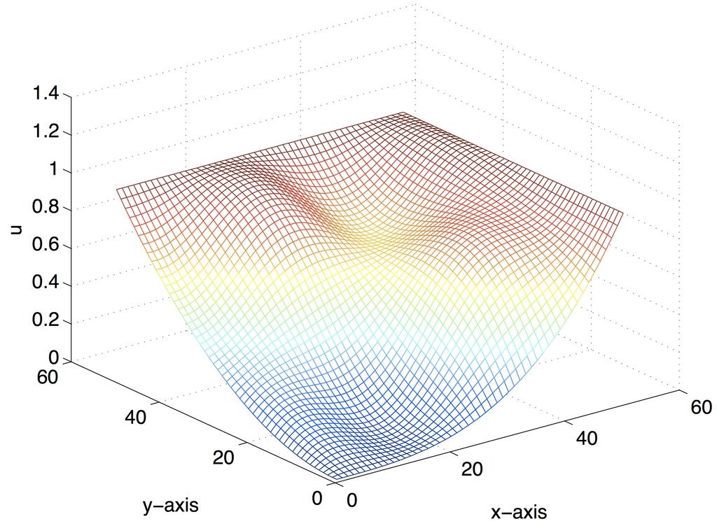
29 Example

30 2D Poisson Equa9on The right hand side function in MATLAB function f = poisson_rhs(x,y) f = 20*cos(3*pi*X).*sin(2*pi*Y); Dirichlet BCs in MATLAB function G = poisson_bcs(x,y,m) G(:,1) = Y(:,1).^2; % left G(:,M+1) = ones(m+1,1); % right G(1,:) = X(1,:).^3; % bottom G(M+1,:) = ones(1,m+1); % top

31 Neumann Problem Poisson equation (14.3) is to be solved on the square domain subject to Neumann boundary condition where denotes differentiation in the direction of the outward normal to The normal is not well defined at corners of the domain and need not be continuous there. To generate a finite difference approximation of this problem we use the same grid as before and Poisson equation (14.3) is approximated at internal grid points by the five-point stencil.

32 Neumann Problem At vertical boundaries, where Taylor expansions, subtracting the gives us Rearrange to get (14.9)

33 Neumann Problem Along the boundary where (note the negative sign appropriate for the outward normal on this boundary), when this is applied at the grid point and we neglect the remainder term, we obtain or (14.10) This approximation involves the value of U at the fictitious grid point which lies outside the domain D. We write the approximation (14.7) at the boundary points (14.11)

34 Neumann Problem We may eliminate between (14.10) and (14.11) to obtain a difference formula with a four point stencil by rearranging the formula in (14.10) into and substitute this into (14.11) to get (14.12) or (14.13)

35 Neumann Problem Along the boundary or at where now the outward normal is positive or, we obtain (14.14) where we have substitution for the fictitious grid point that lies outside the domain D: (14.15) Similar to the left boundary, the approximation (14.7) at the right boundary becomes (14.16)

36 Neumann Problem = fic44ous point

37 Neumann Problem Equation (14.13) also holds with where we also have which is approximated by at the corner (note the positive sign) (14.17) Combining (14.17) with (14.13) at we find Hence, for the corner point on the left boundary (14.18)

38 Neumann Problem For the bottom point at where the outward normal becomes, the approximation is represented by to get the fictitious point (14.19) Hence at the corner bottom point on the left boundary, substituting (14.12) and (14.19) into (14.7) we get (14.20)

39 Neumann Problem In summary, for Neumann BC we need approximation for for the corner points, which, from the approximation at point

40 Neumann Problem The points outside the boundary on the left are approximated using (14.12). The points outside the boundary on the right are approximated using (14.15). The points outside the boundary on the bottom are approximated using (14.19). The points outside the boundary on the top are approximated using (14.17).

41 Neumann Problem Proceeding in this manner for each of the boundary segments and each corner, we arrive at linear equations for the values of U in the domain and on boundaries. We then should assemble the equations into a matrix form (14.16) where we use the same column-wise ordering as before.

42 where Neumann Problem

43 Neumann Problem The right hand side for F actually is approximated in matrix form where

44 Solve the BVP defined by: Example on a unit square with zero-flux on all boundaries: using second order approximation (central finite difference).

45 Example