INVESTIGATION INTO THE EFFECTS OF VARIABLE ROW SPACING IN BOLTED TIMBER CONNECTIONS SUBJECTED TO REVERSE CYCLIC LOADING CALEB JESSE KNUDSON

Transcription

1 INVESTIGATION INTO THE EFFECTS OF VARIABLE ROW SPACING IN BOLTED TIMBER CONNECTIONS SUBJECTED TO REVERSE CYCLIC LOADING By CALEB JESSE KNUDSON A thesis submitted in partial fulfillment of the requirements for the degree of MASTER OF SCIENCE IN CIVIL ENGINEERING WASHIGNTON STATE UNIVERSITY Department of Civil and Environmental Engineering DECEMBER 26

2 To the Faculty of Washington State University: The members of the Committee appointed to examine the thesis of CALEB JESSE KNUDSON find it satisfactory and recommend that it be accepted. Chair ii

3 ACKNOWLEDGEMENT This research was made possible by financial support provided by the National Research Initiative of the United States Department of Agriculture Cooperative State Research, Education, and Extension Service, grant number In addition, I would like to extend my gratitude to the staff of the Wood Materials and Engineering Lab at Washington State University, in particular David Carradine, who was always willing to drop whatever he was doing and lend his help. I would like to thank my committee chair, Dr. J.D. Dolan, who gave me the opportunity to explore timber engineering, and has always put trust in my ability. Furthermore, I would like to thank my other committee members, Dr. David Pollock and Dr. David Carradine, who have made themselves available throughout this research for the many questions that I ve had along the way. I would also like to thank my parents, Ron and Carol, for their support, and Walt and Dixie Bird, who always kept my pantry stocked with their homemade jam. Very special thanks go to Raney Elaine Folland, who has both put up with me, and given her unwavering love and support throughout my career as a student and the creation of this thesis. iii

4 INVESTIGATION INTO THE EFFECTS OF VARIABLE ROW SPACING IN BOLTED TIMBER CONNECTIONS SUBJECTED TO REVERSE CYCLIC LOADING Abstract by Caleb Jesse Knudson, M.S. Washington State University December 26 Chair: J. Daniel Dolan The effects of variable row spacing in single-shear bolted timber connections subjected to reverse cyclic loading have been determined through this experimental research. A variety of performance characteristics including 5% offset yield strength, capacity and ductility have been examined for tested connections as row spacing varied; their results are addressed herein. Statistical analyses were conducted to determine whether inferences could be made regarding mean values for the ductility ratio, 5% offset yield strength and capacity of tested multiple-bolt connections, as row spacing was increased from 2D to 3D. Bolted connections utilizing three different bolt diameters, four unique connection geometries, and variable row spacing within each connection geometry, were subjected to a displacement controlled loading protocol. The protocol used, which was developed by the CUREE-Caltech Wood frame Project is representative of natural hazard loading. Connections were fabricated in order to achieve specific yield modes based on predictions of the Yield Limit Model in order to determine the validity of this model as row spacing was varied. iv

5 The primary conclusion drawn from the results of this research addresses the current design recommendation for row spacing in bolted timber connections. The 21 NDS (AF&PA, 21) states within the provisions of the Geometry factor (C ) that the minimum row spacing in bolted connections shall be 1.5D. This provision should first, be modified to require minimum row spacing for full design value of 3D. Additionally, a linear reduction should be applied in the same manner as current NDS reductions for end distance and bolt spacing, with minimum row spacing for reduced design value of 1.5D. The predictions provided by the Yield Model were, in many cases, inaccurate. Several factors unaccounted for in the model including end fixity caused by the nut and washer, sliding friction between the members, and bolt tensioning, greatly influence connection yield behavior. The derivation of the model should be expanded to include these factors. v

6 Table of Contents List of Figures...ix List of Tables...xxiii Introduction Background Objectives Significance Thesis Overview... 3 Literature Review Introduction Background Yield Limit Model Group Action Factor Brittle Failure Modes Effects of Row Spacing Cyclic Loading Methods and Materials Introduction Specimen Identification Materials Connection Design Test Equipment Apparatus Design vi

7 3.7 - Test Procedures Cyclic Connection Tests Dowel Embedment Tests Bolt bending Yield Strength Moisture Content Tests Specific Gravity Tests Test Data Analysis Results and Discussion General Mode II Yield Cyclic Test Results Mode III s Yield Cyclic Test Results Mode IV Yield Cyclic Test Results Effects of Row Spacing Ductility Ratio % Offset Yield Connection Capacity Yield Limit Model Mode IV-Yield Limit Model Mode III s -Yield Limit Model Mode II-Yield Limit Model vii

8 NDS Appendix E Comparisons Summary, Conclusions, and Recommendations Summary Conclusions Row Spacing Effects % Offset Yield Strength and Connection Capacity Inferences Connection Ductility Inferences Observed Trends as Row Spacing Increases Yield Limit Model Predictions Yield Limit Model Discussion Appendix E Predictions Design Recommendations Limitations of Research Recommendations for Future Research References Appendix A Cyclic Connection Tests A A1.1 - Predicted Yield Mode IV Configurations A1.2 - Predicted Yield Mode III s Configurations A1.3 - Predicted Yield Mode II Configurations Vita viii

9 List of Figures Figure 2.1: Proportional limit defined in a sample load-displacement plot... 5 Figure 2.2: Single shear yield modes Figure 2.3: Definition of 5% offset yield load Figure 2.4: Illustration of minimum row spacing based on critical section... 2 Figure 3.1: Description of reference system Figure 3.2: Specimen dimension definitions Figure 3.3: String potentiometer placement Figure 3.4: Existing steel test frame Figure 3.5: AutoCAD representation of all fixture elements Figure 3.6: Wood specimen-to-steel side plate connection using Simpson S series screws...35 Figure 3.7: Modified CUREE protocol used for cyclic testing of bolted connections Figure 3.8: Dowel embedment cut-off segment from cyclic testing specimens Figure 3.9: Half-hole (right) and full-hole (left) dowel embedment specimens Figure 3.1: Three-point bolt bending test set-up Figure 3.11: Cantilever bolt bending test set-up Figure 3.12: Bi-linear and envelope curves shown on a typical specimen Figure 3.13: Hysteretic energy and strain energy Figure 4.1: Photograph of Mode II splitting/plug shear failure Figure 4.2: Typical load-deflection plot. Mode II yield; single bolt... 5 Figure 4.3: Photograph of different types of row splitting for a single specimen. Mode II yield; three rows of one bolt ix

10 Figure 4.4: Typical load-deflection plot. Mode II yield; three rows of one bolt Figure 4.5: Photograph of group tear-out. Mode II yield; three rows of three bolts Figure 4.6: Typical load-deflection plot. Mode II yield; three rows of three bolts Figure 4.7: Photograph of typical splitting failure. Mode III s yield; one row of three bolts Figure 4.8: Typical load-deflection plot. Mode III s yield; single bolt Figure 4.9: Photograph of typical splitting. Mode III s yield; three rows of one bolt Figure 4.1: Typical load-deflection plot. Mode III s yield; three rows of one bolt Figure 4.11: Photograph of group tear-out. Mode III s yield, three rows of three bolts Figure 4.12: Typical load-deflection plot. Mode III s yield, three rows of three bolts Figure 4.13: Photograph of necking. Mode IV yield; single bolt Figure 4.14: Typical load-deflection plot. Mode IV Yield; single bolt Figure 4.15: Photograph of bolt failure. Mode IV yield; three rows of one bolt Figure 4.16: Typical load-deflection plot. Mode IV yield; three rows of one bolt Figure 4.17: Photograph of spitting. Mode IV yield; three rows of three bolts Figure 4.18: Typical load-deflection plot. Mode IV yield; three rows of three bolts Figure 4.19: Normalized ductility ratio; 6.4 mm (¼ in.) diameter bolt series Figure 4.2: Normalized ductility ratio; 12.7 mm (½ in.) diameter bolt series Figure 4.21: Normalized ductility ratio; 19.1 mm (¾ in.) diameter bolt series Figure 4.22: Normalized 5% offset yield strength; 6.4 mm (¼ in.) diameter bolt series.. 89 Figure 4.23: Normalized 5% offset yield strength; 12.7 mm (½ in.) diameter bolt series x

11 Figure 4.24: Normalized 5% offset yield strength; 19.1 mm (¾ in.) diameter bolt series Figure 4.25: Normalized connection capacity; 6.4 mm (¼ in.) diameter bolt series Figure 4.26: Normalized connection capacity; 12.7 mm (½ in.) diameter bolt series Figure 4.27: Normalized connection capacity; 19.1 mm (¾ in.) diameter bolt series Figure 4.28a: Mode IV experimental/predicted YLM comparison plot: C1 (SI) Figure 4.28b: Mode IV experimental/predicted YLM comparison plot: C1 (Std.) Figure 4.29a: Mode IV experimental/predicted YLM comparison plot: C2 (SI) Figure 4.29b: Mode IV experimental/predicted YLM comparison plot: C2 (Std.) Figure 4.3a: Mode IV experimental/predicted YLM comparison plot: C4 (SI) Figure 4.3b: Mode IV experimental/predicted YLM comparison plot: C4 (Std.) Figure 4.31a: Mode IV experimental/predicted YLM comparison plot: C5 (SI) Figure 4.31b: Mode IV experimental/predicted YLM comparison plot: C5 (Std.) Figure 4.32a: Mode IV experimental/predicted YLM comparison plot: C8 (SI) Figure 4.32b: Mode IV experimental/predicted YLM comparison plot: C8 (Std.) Figure 4.33a: Mode IV experimental/predicted YLM comparison plot: C9 (SI) Figure 4.33b: Mode IV experimental/predicted YLM comparison plot: C9 (Std.) Figure 4.34a: Mode III s experimental/predicted YLM comparison plot: C11 (SI) Figure 4.34b: Mode III s experimental/predicted YLM comparison plot: C11 (Std.) Figure 4.35a: Mode III s experimental/predicted YLM comparison plot: C12 (SI) Figure 4.35b: Mode III s experimental/predicted YLM comparison plot: C12 (Std.) Figure 4.36a: Mode III s experimental/predicted YLM comparison plot: C14 (SI) Figure 4.36b: Mode III s experimental/predicted YLM comparison plot: C14 (Std.) xi

12 Figure 4.37a: Mode III s experimental/predicted YLM comparison plot: C15 (SI) Figure 4.37b: Mode III s experimental/predicted YLM comparison plot: C15 (Std.) Figure 4.38a: Mode III s experimental/predicted YLM comparison plot: C16 (SI) Figure 4.38b: Mode III s experimental/predicted YLM comparison plot: C16 (Std.) Figure 4.39a: Mode III s experimental/predicted YLM comparison plot: C18 (SI) Figure 4.39b: Mode III s experimental/predicted YLM comparison plot: C18 (Std.) Figure 4.4a: Mode III s experimental/predicted YLM comparison plot: C19 (SI) Figure 4.4b: Mode III s experimental/predicted YLM comparison plot: C19 (Std.) Figure 4.41a: Mode II experimental/predicted YLM comparison plot: C21 (SI) Figure 4.41b: Mode II experimental/predicted YLM comparison plot: C21 (Std.) Figure 4.42a: Mode II experimental/predicted YLM comparison plot: C22 (SI) Figure 4.42b: Mode II experimental/predicted YLM comparison plot: C22 (Std.) Figure 4.43a: Mode II experimental/predicted YLM comparison plot: C24 (SI) Figure 4.43b: Mode II experimental/predicted YLM comparison plot: C24 (Std.) Figure 4.44a: Mode II experimental/predicted YLM comparison plot: C25 (SI) Figure 4.44b: Mode II experimental/predicted YLM comparison plot: C25 (Std.) Figure 4.45a: Mode II experimental/predicted YLM comparison plot: C28 (SI) Figure 4.45b: Mode II experimental/predicted YLM comparison plot: C28 (Std.) Figure 4.46a: Mode II experimental/predicted YLM comparison plot: C29 (SI) Figure 4.46b: Mode II experimental/predicted YLM comparison plot: C29 (Std.) Figure 4.47a: Mode II experimental/predicted YLM comparison plot: C3 (SI) Figure 4.47b: Mode II experimental/predicted YLM comparison plot: C3 (Std.) Figure A.1: Mean envelope curve: Configuration xii

13 Figure A.2: Load-Deflection plot: C Figure A.3: Load-Deflection plot: C Figure A.4: Load-Deflection plot: C Figure A.5: Load-Deflection plot: C Figure A.7: Load-Deflection plot: C Figure A.8: Load-Deflection plot: C Figure A.9: Load-Deflection plot: C Figure A.1: Load-Deflection plot: C Figure A.11: Load-Deflection plot: C Figure A.12: Mean envelope curve: Configuration Figure A.13: Load-Deflection plot: C Figure A.14: Load-Deflection plot: C Figure A.15: Load-Deflection plot: C Figure A.16: Load-Deflection plot: C Figure A.17: Load-Deflection plot: C Figure A.18: Load-Deflection plot: C Figure A.19: Load-Deflection plot: C Figure A.2: Load-Deflection plot: C Figure A.21: Load-Deflection plot: C Figure A.22: Load-Deflection plot: C Figure A.23: Mean envelope curve: Configuration Figure A.24: Load-Deflection plot: C Figure A.25: Load-Deflection plot: C xiii

14 Figure A.26: Load-Deflection plot: C Figure A.27: Load-Deflection plot: C Figure A.28: Load-Deflection plot: C Figure A.29: Load-Deflection plot: C Figure A.3: Load-Deflection plot: C Figure A.31: Load-Deflection plot: C Figure A.32: Load-Deflection plot: C Figure A.33: Load-Deflection plot: C Figure A.34: Mean envelope curve: Configuration Figure A.35: Load-Deflection plot: C Figure A.36: Load-Deflection plot: C Figure A.37: Load-Deflection plot: C Figure A.38: Load-Deflection plot: C Figure A.39: Load-Deflection plot: C Figure A.4: Load-Deflection plot: C Figure A.41: Load-Deflection plot: C Figure A.42: Load-Deflection plot: C Figure A.43: Load-Deflection plot: C Figure A.44: Load-Deflection plot: C Figure A.45: Mean envelope curve: Configuration Figure A.46: Load-Deflection plot: C Figure A.47: Load-Deflection plot: C Figure A.48: Load-Deflection plot: C xiv

15 Figure A.49: Load-Deflection plot: C Figure A.5: Load-Deflection plot: C Figure A.51: Load-Deflection plot: C Figure A.52: Load-Deflection plot: C Figure A.53: Load-Deflection plot: C Figure A.54: Load-Deflection plot: C Figure A.55: Load-Deflection plot: C Figure A.56: Mean envelope curve: Configuration Figure A.57: Load-Deflection plot: C Figure A.58: Load-Deflection plot: C Figure A.59: Load-Deflection plot: C Figure A.6: Load-Deflection plot: C Figure A.61: Load-Deflection plot: C Figure A.62: Load-Deflection plot: C Figure A.63: Load-Deflection plot: C Figure A.64: Load-Deflection plot: C Figure A.65: Load-Deflection plot: C Figure A.66: Load-Deflection plot: C Figure A.67: Mean envelope curve: Configuration Figure A.68: Load-Deflection plot: C Figure A.69: Load-Deflection plot: C Figure A.7: Load-Deflection plot: C Figure A.71: Load-Deflection plot: C xv

16 Figure A.72: Load-Deflection plot: C Figure A.73: Load-Deflection plot: C Figure A.74: Load-Deflection plot: C Figure A.75: Load-Deflection plot: C Figure A.76: Load-Deflection plot: C Figure A.77: Load-Deflection plot: C Figure A.78: Mean envelope curve: Configuration Figure A.79: Load-Deflection plot: C Figure A.8: Load-Deflection plot: C Figure A.81: Load-Deflection plot: C Figure A.82: Load-Deflection plot: C Figure A.83: Load-Deflection plot: C Figure A.84: Load-Deflection plot: C Figure A.85: Load-Deflection plot: C Figure A.86: Load-Deflection plot: C Figure A.87: Load-Deflection plot: C Figure A.88: Load-Deflection plot: C Figure A.89: Mean envelope curve: Configuration Figure A.9: Load-Deflection plot: C Figure A.91: Load-Deflection plot: C Figure A.92: Load-Deflection plot: C Figure A.93: Load-Deflection plot: C Figure A.94: Load-Deflection plot: C xvi

17 Figure A.95: Load-Deflection plot: C Figure A.96: Load-Deflection plot: C Figure A.97: Load-Deflection plot: C Figure A.98: Load-Deflection plot: C Figure A.99: Load-Deflection plot: C Figure A.1: Mean envelope curve: Configuration Figure A.11: Load-Deflection plot: C Figure A.12: Load-Deflection plot: C Figure A.13: Load-Deflection plot: C Figure A.14: Load-Deflection plot: C Figure A.15: Load-Deflection plot: C Figure A.16: Load-Deflection plot: C Figure A.17: Load-Deflection plot: C Figure A.18: Load-Deflection plot: C Figure A.19: Load-Deflection plot: C Figure A.11: Load-Deflection plot: C Figure A.111: Mean envelope curve: Configuration Figure A.112: Load-Deflection plot: C Figure A.113: Load-Deflection plot: C Figure A.114: Load-Deflection plot: C Figure A.115: Load-Deflection plot: C Figure A.116: Load-Deflection plot: C Figure A.117: Load-Deflection plot: C xvii

18 Figure A.118: Load-Deflection plot: C Figure A.119: Load-Deflection plot: C Figure A.12: Load-Deflection plot: C Figure A.121: Load-Deflection plot: C Figure A.122: Mean envelope curve: Configuration Figure A.123: Load-Deflection plot: C Figure A.124: Load-Deflection plot: C Figure A.125: Load-Deflection plot: C Figure A.126: Load-Deflection plot: C Figure A.127: Load-Deflection plot: C Figure A.128: Load-Deflection plot: C Figure A.129: Load-Deflection plot: C Figure A.13: Load-Deflection plot: C Figure A.131: Load-Deflection plot: C Figure A.132: Load-Deflection plot: C Figure A.133: Mean envelope curve: Configuration Figure A.134: Load-Deflection plot: C Figure A.135: Load-Deflection plot: C Figure A.136: Load-Deflection plot: C Figure A.137: Load-Deflection plot: C Figure A.138: Load-Deflection plot: C Figure A.139: Load-Deflection plot: C Figure A.14: Load-Deflection plot: C xviii

19 Figure A.141: Load-Deflection plot: C Figure A.142: Load-Deflection plot: C Figure A.143: Mean envelope curve: Configuration Figure A.144: Load-Deflection plot: C Figure A.145: Load-Deflection plot: C Figure A.146: Load-Deflection plot: C Figure A.147: Load-Deflection plot: C Figure A.148: Load-Deflection plot: C Figure A.149: Load-Deflection plot: C Figure A.15: Load-Deflection plot: C Figure A.151: Load-Deflection plot: C Figure A.152: Load-Deflection plot: C Figure A.153: Load-Deflection plot: C Figure A.154: Mean envelope curve: Configuration Figure A.155: Load-Deflection plot: C Figure A.156: Load-Deflection plot: C Figure A.157: Load-Deflection plot: C Figure A.158: Load-Deflection plot: C Figure A.159: Load-Deflection plot: C Figure A.16: Load-Deflection plot: C Figure A.161: Load-Deflection plot: C Figure A.162: Load-Deflection plot: C Figure A.163: Load-Deflection plot: C xix

20 Figure A.164: Load-Deflection plot: C Figure A.165: Mean envelope curve: Configuration Figure A.166: Load-Deflection plot: C Figure A.167: Load-Deflection plot: C Figure A.168: Load-Deflection plot: C Figure A.169: Load-Deflection plot: C Figure A.17: Load-Deflection plot: C Figure A.171: Load-Deflection plot: C Figure A.172: Load-Deflection plot: C Figure A.173: Load-Deflection plot: C Figure A.174: Load-Deflection plot: C Figure A.175: Load-Deflection plot: C Figure A.176: Mean envelope curve: Configuration Figure A.177: Load-Deflection plot: C Figure A.178: Load-Deflection plot: C Figure A.179: Load-Deflection plot: C Figure A.18: Load-Deflection plot: C Figure A.181: Load-Deflection plot: C Figure A.182: Load-Deflection plot: C Figure A.183: Load-Deflection plot: C Figure A.184: Load-Deflection plot: C Figure A.185: Load-Deflection plot: C Figure A.186: Load-Deflection plot: C xx

21 Figure A.187: Mean envelope curve: Configuration Figure A.188: Load-Deflection plot: C Figure A.189: Load-Deflection plot: C Figure A.19: Load-Deflection plot: C Figure A.191: Load-Deflection plot: C Figure A.192: Load-Deflection plot: C Figure A.193: Load-Deflection plot: C Figure A.194: Load-Deflection plot: C Figure A.195: Load-Deflection plot: C Figure A.196: Load-Deflection plot: C Figure A.197: Load-Deflection plot: C Figure A.198: Mean envelope curve: Configuration Figure A.199: Load-Deflection plot: C Figure A.2: Load-Deflection plot: C Figure A.21: Load-Deflection plot: C Figure A.22: Load-Deflection plot: C Figure A.23: Load-Deflection plot: C Figure A.24: Load-Deflection plot: C Figure A.25: Load-Deflection plot: C Figure A.26: Load-Deflection plot: C Figure A.27: Load-Deflection plot: C Figure A.28: Load-Deflection plot: C Figure A.29: Mean envelope curve: Configuration xxi

22 Figure A.21: Load-Deflection plot: C Figure A.211: Load-Deflection plot: C Figure A.212: Load-Deflection plot: C Figure A.213: Load-Deflection plot: C Figure A.214: Load-Deflection plot: C Figure A.215: Load-Deflection plot: C Figure A.216: Load-Deflection plot: C Figure A.217: Load-Deflection plot: C Figure A.218: Load-Deflection plot: C Figure A.219: Load-Deflection plot: C xxii

23 List of Tables Table 3.1: Summary of joint assemblies tested Table 3.2: Summary of specimen dimensions Table 4.1a: Average connection performance results for Mode II yield predictions (SI).55 Table 4.1b: Average connection performance results for Mode II yield predictions (Std.) Table 4.2a: Average connection material properties for Mode II yield predictions (SI)..57 Table 4.2b: Average connection material properties for Mode II yield predictions (Std.) Table 4.3a: Average connection performance results for Mode III s yield predictions (SI) Table 4.3b: Average connection performance results for Mode III s yield predictions (Std.) Table 4.4a: Average connection material properties for Mode III s yield predictions (SI) Table 4.4b: Average connection material properties for Mode III s yield predictions (Std.) Table 4.5a: Average connection performance results for Mode IV yield predictions (SI) Table 4.5b: Average connection performance results for Mode IV yield predictions (Std.) Table 4.6a: Average connection material properties for Mode IV yield predictions (SI).77 xxiii

24 Table 4.6b: Average connection material properties for Mode IV yield predictions (Std.) Table 4.7: Tested and normalized ductility ratio data; predicted Mode IV yield Table 4.8: Statistical inferences concerning means; predicted Mode IV yield Table 4.9: Tested and normalized ductility ratio data; predicted Mode III s yield Table 4.1: Statistical inferences concerning means; predicted Mode III s yield Table 4.11: Tested and normalized ductility ratio data; predicted Mode II yield Table 4.12: Statistical inferences concerning means; predicted Mode II yield Table 4.13a: Tested 5% offset yield data; predicted Mode IV yield (N) Table 4.13b: Tested 5% offset yield data; predicted Mode IV yield (lbs) Table 4.13c: Normalized 5% offset yield data; predicted Mode IV yield Table 4.14: Statistical inferences concerning means; predicted Mode IV yield Table 4.15a: Tested 5% offset yield data; predicted Mode III s yield (N) Table 4.15b: Tested 5% offset yield data; predicted Mode III s yield (lbs) Table 4.15c: Normalized 5% offset yield data; predicted Mode III s yield... 9 Table 4.16: Statistical inferences concerning means; predicted Mode III s yield Table 4.17a: Tested 5% offset yield data; predicted Mode II yield (N) Table 4.17b: Tested 5% offset yield data; predicted Mode II yield (lbs.) Table 4.17c: Normalized 5% offset yield data; predicted Mode II yield Table 4.18: Statistical inferences concerning means; predicted Mode II yield Table 4.19a: Tested connection capacity data; predicted Mode IV yield (N) Table 4.19b: Tested connection capacity data; predicted Mode IV yield (lbs.) Table 4.19c: Normalized connection capacity data; predicted Mode IV yield xxiv

25 Table 4.2: Statistical inferences concerning means; predicted Mode IV yield Table 4.21a: Tested connection capacity data; predicted Mode III s yield (N) Table 4.21b: Tested connection capacity data; predicted Mode III s yield (lbs.) Table 4.21c: Normalized connection capacity data; predicted Mode III s yield Table 4.22: Statistical inferences concerning means; predicted Mode III s yield Table 4.23a: Tested connection capacity data; predicted Mode II yield (N) Table 4.23b: Tested connection capacity data; predicted Mode II yield (lbs.) Table 4.23c: Normalized connection capacity data; predicted Mode II yield Table 4.24: Statistical inferences concerning means; predicted Mode II yield Table 4.25a: Dowel embedment experimental/predicted results (kpa)...14 Table 4.25b: Dowel embedment experimental/predicted results (psi) Table 4.26a: F yb Results (SI)...15 Table 4.26b: F yb Results (Std.) Table 4.27a: Mode IV experimental/predicted YLM comparison: C1 (SI) Table 4.27b: Mode IV experimental/predicted YLM comparison: C1 (Std.) Table 4.28: Inferences concerning means, predicted Mode IV yield: C Table 4.29a: Mode IV experimental/predicted YLM comparison: C2 (SI) Table 4.29b: Mode IV experimental/predicted YLM comparison: C2 (Std.) Table 4.3: Inferences concerning means, predicted mode IV yield: C Table 4.31a: Mode IV experimental/predicted YLM comparison: C4 (SI) Table 4.31b: Mode IV experimental/predicted YLM comparison: C4 (Std.) Table 4.32: Inferences concerning means, predicted mode IV yield: C Table 4.33a: Mode IV experimental/predicted YLM comparison: C5 (SI) xxv

26 Table 4.33b: Mode IV experimental/predicted YLM comparison: C5 (Std.) Table 4.34: Inferences concerning means, predicted mode IV yield: C Table 4.35a: Mode IV experimental/predicted YLM comparison: C8 (SI) Table 4.35b: Mode IV experimental/predicted YLM comparison: C8 (Std.) Table 4.36: Inferences concerning means, predicted mode IV yield: C Table 4.37a: Mode IV experimental/predicted YLM comparison: C9 (SI) Table 4.37b: Mode IV experimental/predicted YLM comparison: C9 (Std.) Table 4.38: Inferences concerning means, predicted mode IV yield: C Table 4.39a: Mode III s experimental/predicted YLM comparison: C11 (SI) Table 4.39b: Mode III s experimental/predicted YLM comparison: C11 (Std.) Table 4.4: Inferences concerning means, predicted Mode III s yield: C Table 4.41a: Mode III s experimental/predicted YLM comparison: C12 (SI) Table 4.41b: Mode III s experimental/predicted YLM comparison: C12 (Std.) Table 4.42: Inferences concerning means, predicted Mode III s yield: C Table 4.43a: Mode III s experimental/predicted YLM comparison: C14 (SI) Table 4.43b: Mode III s experimental/predicted YLM comparison: C14 (Std.) Table 4.44: Inferences concerning means, predicted Mode III s yield: C Table 4.45a: Mode III s experimental/predicted YLM comparison: C15 (SI) Table 4.45b: Mode III s experimental/predicted YLM comparison: C15 (Std.) Table 4.46: Inferences concerning means, predicted Mode III s yield: C Table 4.47a: Mode III s experimental/predicted YLM comparison: C16 (SI) Table 4.47b: Mode III s experimental/predicted YLM comparison: C16 (Std.) Table 4.48: Inferences concerning means, predicted Mode III s yield: C xxvi

27 Table 4.49a: Mode III s experimental/predicted YLM comparison: C18 (SI) Table 4.49b: Mode III s experimental/predicted YLM comparison: C18 (Std.) Table 4.5: Inferences concerning means, predicted Mode III s yield: C Table 4.51a: Mode III s experimental/predicted YLM comparison: C19 (SI) Table 4.51b: Mode III s experimental/predicted YLM comparison: C19 (Std.) Table 4.52: Inferences concerning means, predicted Mode III s yield: C Table 4.53a: Mode II experimental/predicted YLM comparison: C21 (SI) Table 4.53b: Mode II experimental/predicted YLM comparison: C21 (Std.) Table 4.54: Inferences concerning means, predicted Mode II yield: C Table 4.55a: Mode II experimental/predicted YLM comparison: C22 (SI) Table 4.55b: Mode II experimental/predicted YLM comparison: C22 (Std.) Table 4.56: Inferences concerning means, predicted Mode II yield: C Table 4.57a: Mode II experimental/predicted YLM comparison: C24 (SI) Table 4.57b: Mode II experimental/predicted YLM comparison: C24 (Std.) Table 4.58: Inferences concerning means, predicted Mode II yield: C Table 4.59a: Mode II experimental/predicted YLM comparison: C25 (SI) Table 4.59b: Mode II experimental/predicted YLM comparison: C25 (Std.) Table 4.6: Inferences concerning means, predicted Mode II yield: C Table 4.61a: Mode II experimental/predicted YLM comparison: C28 (SI) Table 4.61b: Mode II experimental/predicted YLM comparison: C28 (Std.) Table 4.62: Inferences concerning means, predicted Mode II yield: C Table 4.63a: Mode II experimental/predicted YLM comparison: C29 (SI) Table 4.63b: Mode II experimental/predicted YLM comparison: C29 (Std.) xxvii

28 Table 4.64: Inferences concerning means, predicted Mode II yield: C Table 4.65a: Mode II experimental/predicted YLM comparison: C3 (SI) Table 4.65b: Mode II experimental/predicted YLM comparison: C3 (Std.) Table 4.66: Inferences concerning means, predicted Mode II yield: C Table 4.67a: Appendix E results (SI) Table 4.67b: Appendix E results (Std.) Table 5.1: Optimal connection performance Table 5.2: Summary of YM predictions and observed yield modes Table A.1a: Connection performance properties (SI), Configuration Table A.1b: Connection performance properties (Std.), Configuration Table A.2a: Member properties (SI), Configuration Table A.2b: Member properties (Std.), Configuration Table A.3a: Hysteretic connection properties (SI), Configuration Table A.3b: Hysteretic connection properties (Std.), Configuration Table A.4a: Connection performance properties (SI), Configuration Table A.4b: Connection performance properties (Std.), Configuration Table A.5a: Member properties (SI), Configuration Table A.5b: Member properties (Std.), Configuration Table A.6a: Hysteretic connection properties (SI), Configuration Table A.6b: Hysteretic connection properties (Std.), Configuration Table A.7a: Connection performance properties (SI), Configuration Table A.7b: Connection performance properties (Std.), Configuration Table A.8a: Member properties (SI), Configuration xxviii

29 Table A.8b: Member properties (Std.), Configuration Table A.9a: Hysteretic connection properties (SI), Configuration Table A.9b: Hysteretic connection properties (Std.), Configuration Table A.1a: Connection performance properties (SI), Configuration Table A.1b: Connection performance properties (Std.), Configuration Table A.11a: Member properties (SI), Configuration Table A.11b: Member properties (Std.), Configuration Table A.12a: Hysteretic connection properties (SI), Configuration Table A.12b: Hysteretic connection properties (Std.), Configuration Table A.13a: Connection performance properties (SI), Configuration Table A.13b: Connection performance properties (Std.), Configuration Table A.14a: Member properties (SI), Configuration Table A.14b: Member properties (Std.), Configuration Table A.15a: Hysteretic connection properties (SI), Configuration Table A.15b: Hysteretic connection properties (Std.), Configuration Table A.16a: Connection performance properties (SI), Configuration Table A.16b: Connection performance properties (Std.), Configuration Table A.17a: Member properties (SI), Configuration Table A.17b: Member properties (Std.), Configuration Table A.18a: Hysteretic connection properties (SI), Configuration Table A.18b: Hysteretic connection properties (Std.), Configuration Table A.19a: Connection performance properties (SI), Configuration Table A.19b: Connection performance properties (Std.), Configuration xxix

30 Table A.2a: Member properties (SI), Configuration Table A.2b: Member properties (Std.), Configuration Table A.21a: Hysteretic connection properties (SI), Configuration Table A.21b: Hysteretic connection properties (Std.), Configuration Table A.22a: Connection performance properties (SI), Configuration Table A.22b: Connection performance properties (Std.), Configuration Table A.23a: Member properties (SI), Configuration Table A.24a: Hysteretic connection properties (SI), Configuration Table A.24b: Hysteretic connection properties (Std.), Configuration Table A.25a: Connection performance properties (SI), Configuration Table A.25b: Connection performance properties (Std.), Configuration Table A.26a: Member properties (SI), Configuration Table A.26b: Member properties (Std.), Configuration Table A.27a: Hysteretic connection properties (SI), Configuration Table A.27b: Hysteretic connection properties (Std.), Configuration Table A.28a: Connection performance properties (SI), Configuration Table A.28b: Connection performance properties (Std.), Configuration Table A.29a: Member properties (SI), Configuration Table A.29b: Member properties (Std.), Configuration Table A.3a: Hysteretic connection properties (SI), Configuration Table A.3b: Hysteretic connection properties (Std.), Configuration Table A.31a: Connection performance properties (SI), Configuration Table A.31b: Connection performance properties (Std.), Configuration xxx

31 Table A.32a: Member properties (SI), Configuration Table A.32b: Member properties (Std.), Configuration Table A.33a: Hysteretic connection properties (SI), Configuration Table A.33b: Hysteretic connection properties (Std.), Configuration Table A.34a: Connection performance properties (SI), Configuration Table A.34b: Connection performance properties (Std.), Configuration Table A.35a: Member properties (SI), Configuration Table A.35b: Member properties (Std.), Configuration Table A.36a: Hysteretic connection properties (SI), Configuration Table A.36b: Hysteretic connection properties (Std.), Configuration Table A.37a: Connection performance properties (SI), Configuration Table A.37b: Connection performance properties (Std.), Configuration Table A.38a: Member properties (SI), Configuration Table A.38b: Member properties (Std.), Configuration Table A.39a: Hysteretic connection properties (SI), Configuration Table A.39b: Hysteretic connection properties (Std.), Configuration Table A.4a: Connection performance properties (SI), Configuration Table A.4b: Connection performance properties (Std.), Configuration Table A.41a: Member properties (SI), Configuration Table A.41b: Member properties (Std.): Configuration Table A.42a: Hysteretic connection properties (SI), Configuration Table A.42b: Hysteretic connection properties (Std.), Configuration Table A.43a: Connection performance properties (SI), Configuration xxxi

32 Table A.43b: Connection performance properties (Std.), Configuration Table A.44a: Member properties (SI), Configuration Table A.44b: Member properties (Std.), Configuration Table A.45a: Hysteretic connection properties (SI), Configuration Table A.45b: Hysteretic connection properties (Std.), Configuration Table A.46a: Connection performance properties (SI), Configuration Table A.46b: Connection performance properties (Std.), Configuration Table A.47a: Member properties (SI), Configuration Table A.47b: Member properties (Std.), Configuration Table A.48a: Hysteretic connection properties (SI), Configuration Table A.48b: Hysteretic connection properties (Std.), Configuration Table A.49a: Connection performance properties (SI), Configuration Table A.49b: Connection performance properties (Std.), Configuration Table A.5a: Member properties (SI), Configuration Table A.5b: Member properties (Std.), Configuration Table A.51a: Hysteretic connection properties (SI), Configuration Table A.51b: Hysteretic connection properties (Std.), Configuration Table A.52a: Connection performance properties (SI), Configuration Table A.52b: Connection performance properties (Std.), Configuration Table A.53a: Member properties (SI), Configuration Table A.53b: Member properties (Std.), Configuration Table A.54a: Hysteretic connection properties (SI), Configuration Table A.54b: Hysteretic connection properties (Std.), Configuration xxxii

33 Table A.55a: Connection performance properties (SI), Configuration Table A.55b: Connection performance properties (Std.), Configuration Table A.56a: Member properties (SI), Configuration Table A.56b: Member properties (Std.), Configuration Table A.57a: Hysteretic connection properties (SI), Configuration Table A.57b: Hysteretic connection properties (Std.), Configuration Table A.58a: Connection performance properties (SI), Configuration Table A.58b: Connection performance properties (Std.), Configuration Table A.59a: Member properties (SI), Configuration Table A.59b: Member properties (Std.), Configuration Table A.6a: Hysteretic connection properties (SI), Configuration Table A.6b: Hysteretic connection properties (Std.), Configuration xxxiii

34 Introduction Background Bolted connections are very common in wood design. They are straight forward to design, and relatively simple to install on site. The responses of single-bolt timber connections to monotonic loading conditions are well understood, however, the behavior of bolted timber connections utilizing multiple-bolt configurations is not as well defined, particularly for connections subjected to cyclic loading conditions, such as those imposed by hurricane and earthquake forces. Traditionally, bolted connection design has been based on monotonic load application and working stress levels. More specifically, designs were conducted so that the load induced would not exceed the proportional limit of a connection. Monotonic loading is representative of the type of load experienced during sustained dead or live loads. It has been assumed in design that a structure will respond in much the same manner when exposed to events such as high wind or earthquake as it will to sustained loading. Current design criterion for dowel-type connection design in the 21 National Design Specification (NDS (AF&PA, 21)) is based on the Yield Model, which was developed by European researchers in the mid-twentieth century. The minimum requirement for row spacing in bolted timber connections loaded parallel to grain is one and a half times the bolt diameter (1.5D) as recommended by early researchers. Over the past two decades, much research has been conducted in order to achieve a better understanding of the behavior of bolted connections when exposed to natural hazard loading. Technology had governed earlier research; however, recently, methods 1

35 have been developed to allow simulated testing of dynamic forces imposed by earthquakes and high wind in a controlled laboratory environment. To gain better understanding of multiple-bolt connection behavior under natural hazard loading, the primary objective of this research is to determine the effects of row spacing on the performance of bolted timber connections when subjected to cyclic loading conditions. Additionally, it is of interest to determine if current NDS recommendations for row spacing are adequate Objectives The objectives of this research include: Quantifying the effect of variable row spacing on bolted connection strength characteristics including connection capacity, 5% offset yield strength, and ductility ratio. Identifying any apparent trends in connection performance as row spacing is varied and either proving or disproving them with statistical analyses. Determining the validity of the Yield Model s strength and yield mode predictions for variable row spacing in multiple-bolt connections exposed to cyclic loading. Quantifying additional connection performance parameters including stiffness, equivalent elastic plastic yield, equivalent viscous damping, hysteretic energy, displacement capacity, and strain energy for different multiple-bolt configurations. 2

36 1.3 - Significance The current minimum row spacing recommended by the NDS (AF&PA, 21) is one and a half times the diameter of the bolt (1.5D). This research will determine if the recommended row spacing is acceptable for multiple-bolt connections subjected to earthquake or high wind loading, or if alternate minimum row spacing should be considered for multiple-bolt connections Thesis Overview Chapter Two presents a literature review of past research conducted, which is considered relative to multiple-bolt connections subjected to reverse cyclic loading. The experimental procedures used in this research concerning full connection tests and all secondary testing are described in Chapter Three. Chapter Four presents and discusses results of this research based on raw data and statistical analyses; followed by Chapter Five which presents a summary of this research and conclusions drawn from its results. Finally, Appendix A presents load-deflection plots from cyclic testing along with raw data from a variety of strength and serviceability parameter analyses. 3

37 Literature Review Introduction Forces imposed on timber structures from wind and earthquake events are the primary sources of lateral loading, and in timber construction, the majority of lateral loads are resisted by the connections. There is a large degree of uncertainty when addressing earthquakes pertaining to their magnitude and manner in which the resulting force is applied to a structure. Since it is not possible to control natural hazards, we must attain a better understanding of timber structure behavior when subjected to seismic loading, so that the design process considers a careful balance of strength, stiffness, and ductility (Popovski et al., 22). Relatively inexpensive and easy to install, bolts are a common fastener type used in timber connections. The behavior of bolted joints is highly variable based on the number of members connected, total bolt quantity, and connection geometry. The connection may be described as either a single-shear or a multiple-shear configuration, depending on the number of member interfaces. Bolted timber connections utilize either a single-bolt or multiple-bolt configuration. Single-bolt connections consist of a single bolt, whereas multiple-bolt connections feature multiple rows and/or multiple-bolts per row, with a row of bolts being defined as a line of bolts, parallel to the direction of the applied load. Connection geometry is based not only on the total number of bolts used, but on edge distance, end distance, bolt spacing, and row spacing of a connection. 4

38 2.2 - Background The basis for recommendations used in current United States connection design philosophies can be traced back to research conducted by George Trayer (1932). Trayer performed several hundred connection tests utilizing different hardwood and softwood species with various bolt diameters and lengths. Additionally, load was applied both parallel and perpendicular to grain with varied connection geometries. From these tests, Trayer made recommendations for various connection parameters, and defined the proportional limit as the average stress under the bolt when the slip ceases to be proportional to the load being applied (Trayer, 1932). This concept is illustrated in Figure 2.1. Trayer s research is significant because it formed the basis for allowable bolt strengths used in U.S. timber design codes for many years to come (Moss, 1996). Load Proportional Limit Load Displacement (Slip) Figure 2.1: Proportional limit defined in a sample load-displacement plot. The proportional limit load, as defined by Trayer, was the basis for allowable bolted timber connection design loads starting with the National Design Specification for 5

39 Stress Grade Lumber and its Fasteners (NLMA, 1944), continuing through the 1986 National Design Specification for Wood Construction (AF&PA, 1986). In the 1991 National Design Specification for Wood Construction (AF&PA, 1991), a mechanics based set of equations developed by European researchers was adopted to calculate bolted timber connection design values. The equations, referred to as the Yield Model, predict yield strength for dowel type connections based on dowel bearing strength of the wood, and fastener bending yield strength (Soltis and Wilkinson, 1991). The Yield Model is the current basis for determining bolted timber connection yield strength in the National Design Specification for Wood Construction (AF&PA, 21) and will be discussed in detail in the following section. The Yield Model is limited however, in that it only considers yielding of connections containing a single bolt, and does not consider brittle failure modes of single or multiple-bolt connections such as splitting or group tear-out. The 21 National Design Specification does however include provisions to address the issue of failure in bolted timber connections. Non-mandatory Appendix E, Local Stresses in Fastener Groups (AF&PA, 21) provides a series of equations based on mechanical strength properties of wood members and connection geometry to determine the ultimate capacity of multiple-bolt timber connections. The appendix equations provide a means of determining capacities for net-section tension rupture, row tear-out, and group tear-out, and will be discussed in detail later in this chapter. 6

40 2.3 - Yield Limit Model The NDS Yield Model (YM) is derived from the European Yield Model (EYM) introduced by Johansen (1949), and predicts the lateral strength of a single dowel-type fastener connection (McLain, 1991). The YM also provides a description of possible bolt yield modes that can occur in timber connections. Yield strengths for the different modes are based on equilibrium equations resulting from free body diagrams of a bolt in a wood member. The yield mode resulting in the lowest yield load for a given connection will be the yield load for that connection (Patton-Mallory, 1991) and (Wilkinson, 1993). The four possible single-shear yield modes are shown in Figure 2.2 Yield Mode I Yield Mode II Yield Mode III Yield Mode IV Figure 2.2: Single shear yield modes. 7

41 The four yield modes illustrated in Figure 2.2 encompass a total of six descriptions and design equations. Yield Mode I, and Yield Mode III have slight differences according to which member experiences yielding, and are subdivided into either side or main member yield. The 21 NDS (AF&PA, 21) Yield Limit modes are described as follows: Yield Mode I Yield Mode II Wood crushing in either the main or the side member. Localized wood crushing near the faces of the wood members based on rotation of a rigid fastener about the shear plane. Yield Mode III - Fastener yield in bending at one plastic hinge point per shear plane and associated localized wood crushing. Yield Mode IV Fastener yield in bending at two plastic hinge points per shear plane and associated localized wood crushing. Equations for the yield limit modes as used in the 21 NDS (AF&PA, 21) are presented below. The yield load of a connection is taken as the lowest value calculated from each equation. A subscript of m denotes yielding occurring in the main member, and a subscript of s denotes yielding in the side member. Yield Modes: Z Im Dlm F R d em (2.1) Z Is Dls F R d es (2.2) 1 ZII k Dls F R d es (2.3) 8

42 Z IIIm k2dlm Fem (1 2R ) R e d (2.4) Z IIIs k3dls Fem (2 R ) R e d (2.5) Z IV D R 2 d 2F 3(1 em F yb R ) e (2.6) where: k 1 R e 2R 2 e (1 R t (1 R 2 t ) R ) e R 2 t R 3 e R (1 e R ) t (2.7) k 2 1 2(1 R e ) 2F yb (1 3F 2R e 2 emlm ) D 2 (2.8) k 3 1 2(1 R R e e ) 2F yb (2 3F R ) D e 2 emls 2 (2.9) D = Fastener diameter, in.. F yb = Dowel bending yield strength, psi. F em = Main member dowel bearing strength, psi. F es = Side member dowel bearing strength, psi. l m = Main member dowel bearing length, in.. l s = Side member dowel bearing length, in.. R e = F em /F es. R t = l m /l s. R d = Reduction term based on yield mode and dowel angle to grain. 9

43 Yield Model predictions have been compared to previous experimental research performed by Trayer (1932), Soltis and Wilkinson (1986), and McLain and Thangjtham (1983). Good agreement has been found between the data sets, with the Yield Model predicting slightly conservative values for yield strength in bolted timber joints loaded parallel to grain considering that friction in the joints is neglected. Inherent to the model was the assumption that yield strength would be reached when either the compressive strength of the wood beneath the bolt was exceeded, or one or more plastic hinges formed in the fastener. Several other underlying assumptions have been built into the YM as stated by McLain and Thangjtham (1983), and are listed below: The joint resists an externally applied lateral load through fastener bending resistance, and bearing resistance of the wood member. Bolts and any steel side plates used are homogeneous, isotropic, and elasto-plastic. Wood members are homogeneous, orthotropic and behave elastoplastically when loaded parallel to grain. The effects of shear and tensile stresses in the development of plastic moments are neglected. The ends of the bolts are free to rotate, and bearing stress under the bolt is uniformly distributed with the bolt fitting tightly in the hole. Friction between the members is ignored. Since the development of the YM, modifications have been proposed to allow the model to account for conditions that are more likely to occur in practice. McLain and Thangjtham (1983) proposed modifications that would account for end fixity imposed by 1

44 nuts and washers at the surfaces of timber members. Larsen (1973) introduced a modification to the model that would account for the sliding friction between the timber members of the connection. As listed above, the YM assumes a well-manufactured joint with a nearly perfect fit of the holes. United States design philosophies allow for a maximum bolt-hole over-drill of 1.6 mm (.625 in.) accounting for construction tolerances, which are unaccounted for in the YM. However, a study conducted by Wilkinson (1993) found that increased bolt-hole size had little effect on yield load or maximum load, but generally increased deformation for single-bolt connections. Connection yield strength has been defined differently by various researchers. Prior to U.S. adoption in the 1991 NDS (AF&PA, 1991), the YM predicted that yield strength could potentially be any load on the load-deformation curve (Wilkinson, 1993). This definition of yield strength was not appropriate for the U.S. approach, which was to define a yield strength that enabled repeatability of results (Wilkinson, 1991). The yield load definition adopted into the 21 NDS (AF&PA, 21) is illustrated in Figure 2.3. Yield Load Load 5% of Bolt Diameter Displacement (Slip) Figure 2.3: Definition of 5% offset yield load. 11

45 As illustrated in the previous figure, the yield load is the point at which the load- displacement curve intersects a straight line parallel to the initial linear portion of the curve. This line is offset by 5% of the fastener diameter from the origin of the load- displacement curve (Harding and Fowkes, 1984). Occasionally, when using larger diameter bolts, catastrophic failure will preclude this defined yield point from occurring, in which case, the 5% offset yield strength defines the ultimate load. The same definition is applied to determine dowel bearing yield strength and fastener bending yield strength as stated in ASTM D5764 ASTM (24), and ASTM F1575 ASTM (24) respectively. The yield point as defined above will fall between the proportional limit and the maximum load on the load-displacement curve for all components considered Group Action Factor According to Cramer (1968), Milton in 1885 was the first to note an unequal load distribution in a row of fasteners. He stated that the outermost and innermost rivets of double-butt strap joints transmit a greater proportion of the load than did the intermediate rivets. Doyle and Scholten (1963) expanded this research to include timber joints, and found that the bearing stress in multiple-bolt joints was less on a per-bolt basis than that of single-bolt joint. In 1968, Cramer developed a linear-elastic analytical model to determine load distribution in a row of bolts. His model assumed a frictionless joint with non-uniform stress distribution through the cross-section of the members. Cramer verified this model by testing perfectly machined, butt-type timber joints with varying bolt spacing and number of bolts per row. Fairly good agreement was found between theoretical results 12

46 and experimental results (Cramer, 1968). Cramer did note that bolt-hole misalignment between the main member and splice plates, which was not accounted for in his model, produced an unpredictable load distribution in a row of bolts. Lantos (1969) developed a similar linear-elastic analytical model to determine the load distribution within a row of bolts in timber connections. His model varied from Cramer s in that uniform stress distribution was assumed through the cross-section of a member. It was also assumed that a linear relationship existed between fastener deformation and load (Lantos, 1969). Lantos did not verify his model with experimental testing. In their research, Lantos and Cramer made similar observations regarding rows of bolts. It was assumed that rows of bolts spaced far enough apart would act independently of each other (Cramer, 1968). Lantos (1969) noted that as the number of fasteners per row increases, the proportion of load to a single bolt decreases. Additionally, Lantos found that as the number of rows increased, there was a proportional increase in the strength of the joint. Wilkinson (198) expanded on the research conducted by Lantos and Cramer in an effort to develop a procedure that would account for single-bolt load-slip behavior and fabrication tolerances when determining load distribution in a row of bolts. He compared the model developed by Lantos to his own experimental data, finding that the model gave an accurate prediction of the proportional limit load for a row of fasteners. However, because the model did not consider non-linear behavior, capacity was overestimated. Wilkinson arrived at a similar conclusion to Cramer regarding fastener-hole misalignment between main and side members, stating that any bolt in a row may 13

47 transmit the largest percentage of load on the joint as capacity is approached, or virtually no load (Wilkinson, 198). Prior to the 1973 NDS (AF&PA, 1973), multiple-bolt connection design stated that the allowable load on a group of fasteners is the product of the single-bolt design value and the number of fasteners in the group (Lantos, 1969). Based on research conducted by Lantos (1969), row modification factors were introduced into the 1973 National Design Specification (AF&PA, 1973) to account for load reduction as the number of bolts per row was increased. Zahn (1991) reduced the Lantos model to a single equation, first present in the 1991 NDS (AF&PA, 1991), currently referred to as the group action factor, C g, in the 21 NDS (AF&PA, 21). Current design recommendations by the NDS for multiple-fastener connections utilize the group action factor in conjunction with the nominal design value (Z) as shown in Equation 2.1. Z = n Z C g (2.1) where: C g = [m(1-m 2n 2)] n m m ) [1+R 1 R EA ] (2.11) n[(1+r EA n ) (1+m)-1+m 2n EA Cg n 2] n [1-m] n (1 R m )(1 m) 1 m 1 m EA C g = 1. for dowel type fasteners with D < ¼ in. n = Number of fasteners in row. Es As Em Am R EA = Lesser of or (2.12) E A E A m m E m = Main member modulus of elasticity. E s = Side member modulus of elasticity. A m = Main member gross cross-sectional area. A s = Side member gross cross-sectional area. s s 14

48 m = u-sqrt(u u ( u 2 2-1) 1) (2.13) = + s [ _ _ 1 u 1 2 [ E m A m E s A s (2.14) m m s s s = Center to center spacing between fasteners in a row. = Load/slip modulus; calculated as: [(18.)(D 1.5 )] (lbs. /in.). D = Fastener diameter, in Brittle Failure Modes Current U.S. design philosophies utilize the Yield Model, which is based on 5% offset yield strength. This model has been shown to accurately predict the yield load in single-bolt connections when the joint does not fail from axial load on the net section, and when the edge and end distances are sufficient to prevent failure due to shear or splitting (McLain and Thangjtham, 1983). However, when multiple-bolt connections are considered, the ultimate mode of failure observed could be much different based on the tendency of multiple-bolt timber connections to display brittle failure modes. Considering the Yield Model s inability to accurately predict strength connections displaying brittle failure behavior, it is desirable to evolve toward a capacity based design procedure (Anderson, 21). Capacity is currently defined as the load at which rupture occurs, or the load at a displacement of one inch, whichever occurs first as stated by ASTM D Test Method for Mechanical Fasteners in Wood (ASTM, 24). Connection capacity is affected not only by the wood members physical and mechanical properties, but by the connection geometry as well. Recent research performed by Gutshall (1994), Anderson (21), and Dodson (23) have shown that brittle failure 15

49 modes, including splitting, tension rupture, and group-tear-out are all influenced by connection geometry. The 21 NDS (AF&PA, 21) includes a non-mandatory provision providing capacity checks for connections displaying brittle failure modes including net-section tension rupture, row tear-out, and group tear-out. The non-mandatory provision in the most recent edition of the NDS (AF&PA, 21) takes into account the effects of bolt spacing and row spacing on multiple-bolt connection capacity, and provides a more accurate representation of connection behavior. The brittle failure modes are used much in the same manner as the Yield Model in that the lowest calculated capacity will govern the connection displaying the associated mode of failure. Failure modes, as outlined in the 21 NDS (AF&PA, 21), are described and defined as follows: Net section tension capacity: Occurs when a tension failure perpendicular to the direction of loading occurs at the critical cross-section of the bolted joint. Z ' NT where: F ' t A net Z NT = Allowable tension capacity of net section area. F t = Allowable tension design value parallel to grain. A net = Net cross-sectional area of critical section. (2.15) Row tear-out capacity for a single row of fasteners: Occurs when two shear lines form tangent to the row of bolts parallel to grain. Z ' RTi n F ts i ' v critical (2.16) 16

50 where: Z RTi = Allowable row tear-out capacity of row i. F v = Allowable shear design value parallel to grain. t = Thickness of member. n i = Number of fasteners in row i. s critical = Minimum spacing in row i taken as the lesser of the end distance for the spacing between fasteners in row i. Row tear-out capacity for multiple rows of fasteners: Occurs in the same manner as row tear-out for a single row, but multiple rows are considered. ' n row Z RT Z RTi i 1 ' (2.17) where: Z RT = Allowable row tear-out capacity of connection. n row = Number of rows. Group tear-out capacity: Occurs due to tension rupture perpendicular to the direction of the applied load in the critical section between the two or more rows of bolts in combination with a shear failure line tangent to the outer rows of bolts parallel to the grain of the member. (This type of failure would be analogous to a block shear failure in steel design.) Z ' GT Z RT 2 1' Z RT 2 n' F ' t A group net (2.18) 17

51 where: Z GT = Allowable group tear-out capacity. Z RT-1 = Allowable row tear-out capacity of row 1 of fasteners bounding the critical group area. Z RT-n = Allowable row tear-out capacity of row n of fasteners bounding the critical group area. A group-net = Critical group net-section area between row 1 and row n. Doyle (1964) first noted that multiple-bolt connections loaded in tension would fail by splitting, row tear-out, and group tear-out. While multiple-bolt connections often display brittle failure modes, it should be noted that single-bolt connections may also display brittle failure modes in addition to the ductile failure modes predicted by the YM (Jorissen, 1998). Jorissen (1998) developed a fracture mechanics based model to predict the ultimate load carrying capacity for double-shear joints producing brittle failure. Inherent to the model were the effects of tension parallel and perpendicular to grain, and shear parallel to grain. These factors were found to greatly influence capacity in connections displaying brittle failures. Quenneville and Mohammad (2) tested multiple-bolt connections with variable end distances, bolt spacing and number of bolts per row, row spacing and number of rows, member thickness, and member species. Brittle failure modes including row tear-out, group tear-out, and splitting were observed in connection tests loaded monotonically in tension. Quenneville and Mohammad (2) derived from test 18

52 observations that the most significant material property influencing the capacity of multiple-bolt connections was the member s shear strength. As the above research suggests, shear and tension strengths both perpendicular and parallel to grain have been shown to influence the behavior of bolted connections. It is important note that both single and multiple-bolt connections can display either ductile or brittle failure modes. The YM has been shown to compare favorably with experimental results from single-bolt connection tests displaying ductile behavior, but overestimates the capacities of connections displaying brittle failure. Furthermore, considering that the non-mandatory Appendix E of the NDS (AF&PA, 21) has been shown to underestimate the capacity of a brittle connection as stated by Dodson (23), despite being dependent on the row spacing and bolt spacing of a connection, a better understanding of connection behavior displaying brittle failure is vital Effects of Row Spacing The current recommendation for row spacing in U.S. design philosophies is based on research conducted by Trayer (1932). Based on the results of several hundred tests, Trayer stated that the center-to-center spacing between adjacent rows of bolts was controlled by the reduction in area at the critical section. It was recommended that the net tension area remaining at the critical section, when coniferous woods were used, should be at least 8% of the total area in bearing under all the bolts in the particular timber in question (Trayer, 1932). To better understand the definition that Trayer has given, see Figure

53 Bearing area under bolts: (4) 12.7 mm (½ in.) diameter bolts x 76.2 mm (3 in.) member thickness results in an area of 387 mm 2 (6 in. 2 ). Critical net section area: [Gross width of 11.6 mm (4 in.) - (2) x 12.7 mm (½ in.) diameter bolts] x 76.2 mm (3 in.) thickness results in an area of 586 mm 2 (9 in. 2 ). The connection illustrated below is adequate because the critical net section area is equal to or greater than 8% of the total area in bearing under the bolts. All holes have (½ in.) diameter 4 in. 3 in. Figure 2.4: Illustration of minimum row spacing based on critical section. Trayer s recommendation for row spacing was adopted into the first National Design Specification released (NLMA, 1944). Row spacing requirements were adapted in the 1971 National Design Specification (AF&PA, 1971) to provide an explicit center- 2

54 to-center row spacing for multiple rows connection loaded parallel to grain of not less than one and one half times the diameter of the bolt (1.5D). Quenneville and Mohammad (2) tested 46 steel-wood-steel double-shear tension connections using two different row spacings. It was noted that when a row spacing of 3D was used, the predominant mode of failure was group tear-out, and when a row spacing of 5D was used, the predominant mode of failure was row tear-out. Based on their results, the influence of row spacing on the failure mode and strength of the connection was argued to be very significant (Quenneville and Mohammad, 2). Dodson (23) tested 27 steel-wood-steel double-shear tension connections loaded monotonically parallel to grain. All wood members used in Dodson s testing were Douglas fir glued laminated lumber (glulam). Row spacing was among the connection parameters varied within the different configurations. He found that the relative effects of row spacing appeared to be properly addressed in the NDS 21 Appendix E provisions. Furthermore, failure modes as predicted by Appendix E provisions in the NDS (AF&PA, 21) were predicted with a higher level of accuracy for multiple-bolt connections with larger row spacings when compared to those with smaller row spacings. NDS 21 Appendix E equations did, however, over-predict the ultimate connection capacity. Ultimate test loads were, on average, only half of predicted capacities (Dodson, 23) Cyclic Loading The traditional method for testing timber joints with dowel type fasteners has typically been to apply a monotonic load to the joint in tension. This loading condition, 21

55 referred to as pseudo-static, simulates a static load over a small period of time, by applying a slow load at a constant rate (Anderson, 21). Monotonic tests, however, do not provide adequate information about the behavior of bolted connections based on all loading conditions that they may be exposed to. Earthquake forces and high wind conditions such as hurricanes, may load a structure in an infinite number of planes in alternating directions, resulting in alternating tension and compression forces on a connection. To achieve a better understanding of the behavioral response of bolted timber connections when exposed to wind or earthquake forces, a testing method representative of those forces must be considered. Several cyclic loading protocols have been reviewed and considered for standardization. All protocols described below feature loading patterns that cycle through zero and fully-reverse the force in the member from tension to compression. The Sequential Phased Displacement Protocol (SPD), used by Gutshall (1994), is a proposed ASTM draft standard according to Anderson (21) which employs a loading pattern intended to define conservative estimates for performance and design (Dolan, 1994). The International Standards Organization (ISO) published a standard in 23 entitled Timber Structures Joints made with Mechanical Fasteners Quasi-Static Reversed Cyclic Test Method according to Billings (24). The loading protocol used by Anderson (21), Billings (24), and in the present research was a displacement based protocol developed by the Consortium of Universities for Research in Earthquake Engineering (CUREE) (Krawinkler et. al., 21). The CUREE Protocol was developed to establish common testing protocols for all component tests of the CUREE/Caltech Woodframe Project. The CUREE loading protocol employs cumulative damage concepts to transform time history 22

56 responses into a representative deformation controlled loading history. It is based on a collection of twenty ordinary ground motions recorded in southern California whose probability of exceedance in 5 years is 1 percent (Krawinkler et. al., 21). This allows the seismic performance of a structure to be evaluated based on ordinary ground motions which may precede the capacity level event in addition to ordinary ground motions of the capacity level event. Several studies have been performed to determine the specific influences of dynamic loading relative to pseudo-static loading on the behavior of bolted timber connections. Dynamic loading has been shown to produce load-displacement plots displaying pinched, degrading hysteretic loops (Chun et al., 1996). The hysteretic loops may be used to characterize the performance of a bolted timber connection by the amount of energy that has been dissipated. This characteristic can be obtained from the loaddisplacement plot from a connection test, and is defined as the area enclosed by each hysteresis loop. Popovski et al. (22) tested a variety of timber connections under monotonic and quasi-static cyclic loading. Their study characterized the seismic behavior and failure modes of a variety of connections used in braced timber frames. They found that the behavior in bolted connections was dependent on the slenderness ratio of the bolt. Bolts with low slenderness ratios (length in bearing/bolt diameter) resulted in rigid connections with high local stresses in the wood and, ultimately, brittle failure mechanisms. Conversely, bolts with high slenderness ratios (smaller relative diameter bolts) resulted in more ductile connections. Additionally, energy dissipation in bolted connections with 23

57 small diameter bolts was much greater than for large diameter bolts, which suggested small diameter bolts were more desirable in seismic design (Popovski et al., 22). Quenneville and Mohammad (1998) developed a load driven ramped cyclic loading protocol with a frequency of one cycle per minute. The loading pattern was applied to Spruce-Lodgepole Pine glued laminated timber loaded parallel and perpendicular to grain. Similar failure modes were observed for specimens subjected to cyclic or monotonic loading, however, a larger degree of ductility and associated energy dissipation, defined as the area enclosed by the hysteretic loops, was observed in connections subjected to ramped cyclic loading. Higher residual strength values and lower maximum deflections were observed in connections subjected to the ramped cyclic loading protocol relative to those loaded monotonically. Additionally, the differences in loading regime were less significant when considering single-bolt connections as opposed to multiple-bolt connections (Quenneville and Mohammad, 1998). 24

58 Methods and Materials Introduction In an effort to quantify the effects of row spacing on a variety of strength and serviceability parameters, single-shear multiple-bolt timber connections were subjected to reverse cyclic loading parallel to grain until catastrophic failure occurred in one or both of the members. Twenty connection configurations with different characteristics were considered. Variables within the different connection configurations included bolt diameter, member thickness, number of rows, bolts per row, and row spacing. A summary of the joint assemblies tested is given in Table 3.1. Table 3.1: Summary of joint assemblies tested. Configuration Main Side Bolt Number Bolts Row Member* Member* Diameter Of Rows Per Row Spacing 1 4x4 4x x4 4x mm 4 4x4 4x D (¼ in.) 5 4x4 4x D 8 4x4 4x D 9 4x4 4x D 11 4x4 2x x4 2x x6 2x mm 3 1 2D 15 4x6 2x6 (½ in.) 3 1 3D 16 4x6 2x D 18 4x6 2x D 19 4x6 2x D 21 2x4 2x x4 2x x8 2x mm 3 1 2D 25 2x1 2x1 (¾ in.) 3 1 3D 28 2x8 2x D 29 2x1 2x D 3 2x8 2x D Expected Yield Mode IV III S II *Nominal member dimensions in inches 25

59 Test geometries were selected in order to achieve Yield Modes II, III S, and IV based on 21 NDS (AF&PA, 21) Yield Limit equations. Yield Mode I was excluded from this research as it is only likely to occur if the dowel is tightly fitted, which is not typical in bolted timber construction. Connection capacities were calculated for comparison with test results based on the equations for local stresses in fastener groups given in Appendix E of the 21 NDS (AF&PA, 21). These equations are based on the capacity of the wood surrounding the connection, and include considerations for net section tension capacity, row tear-out capacity, and group tear-out capacity. Secondary tests were conducted in order to obtain dowel embedment strength, bolt bending yield strength, moisture content, and specific gravity. All secondary tests were performed in accordance with ASTM standards as discussed in later sections Specimen Identification The identification reference system used was consistent for both the primary connection and secondary testing. Specimens were identified based on their configuration number from Table 3.1, rather than joint assembly specifics. An example of the reference system is shown in the Figure 3.1 below. C11M5 Configuration Member Specimen Number M = Main S = Side Figure 3.1: Description of reference system. 26

60 3.3 - Materials Lumber used to fabricate all test specimens was kiln dried Douglas Fir-Larch purchased from local suppliers. All 51mm (2-inch) nominal thickness lumber and 12 mm (4-inch) by 152 mm (6-inch) nominal dimension lumber was graded Number 2 and Better, and 12 mm (4-inch) by 12 mm (4-inch) nominal dimension lumber was graded Number 1 and Better. Upon delivery and sizing of each specimen, the lumber was placed in a conditioning chamber for a minimum of 9 days, where the temperature was held at 24 C 1.1 C (75 F 2 F) and 64% 2% relative humidity to equilibrate to approximately 12 % moisture content. Whenever possible, specimens were cut so that main and side members would be cut from the same board and end matched. In doing this, the strength properties and physical characteristics of each member would be similar so that the strength of one member would not necessarily govern over the other in an effort to minimize the effects of local variations within the board. Bolt-holes were drilled 1.6 mm (.625 in.) larger than the bolt diameter using a drill press. The drill press provided an efficient and relatively accurate means for producing the holes, however, due to cupping of some boards, they were not able to rest flush against the surface of the drill press table causing holes to be drilled at a slight angle and bolt-hole misalignment to occur. Where specimens experienced bolt misalignment, the bolts were driven by force as would be done in actual construction. All specimens were cut and bolt-hole locations chosen in order to minimize the effect of knots, checks, splits, etc. in critical sections of the connection. A critical section was defined as any location in which a defect in the wood might significantly reduce the 27

61 strength of the connection. While it was the intent to minimize the occurrence of defects adjacent to the bolt-hole locations and misalignment between the members, neither could be completely eliminated. The error resulting from each was not considered in the analysis or test results. It was assumed that these types of fabrication errors in multiplebolted connections would approximate field conditions Connection Design All members tested were sized so that the 21 NDS (AF&PA, 21) recommendations for distances and spacing were met or exceeded. Bolt spacing and end distance were set at 7D based on preliminary results obtained from an associated project investigating the effect of bolt spacing within a row (Billings, 24). Member widths were chosen so that the edge distance would be equal to or greater than the row spacing, while maintaining the 21 NDS (AF&PA, 21) minimum requirement of 1.5D. All bolts used in the connection tests were ASTM A37 bolts purchased though local suppliers. Bolts with a diameter of 6.4 mm (¼ in.) were used in configurations predicted to yield in Mode IV; bolts with a diameter of 12.7 mm (½ in.) were used in configurations predicted to yield in Mode III S, and bolts with a diameter of 19.1 mm (¾ in.) were used for configurations predicted to yield in Mode II. Bolt lengths were selected so that the threaded portion of the bolt was excluded from the shear plane in all tests. The minimum row spacing for this study was 2D. When considering 6.4 mm (¼ in.) and 12.7 mm (½ in.) bolts in configurations with three rows, the clearance between the rows of bolts was not adequate to accommodate the center row of washers on either side of the connection. 28

62 The washers had to be ground down on opposite sides in order to fit into the connection. Dimensions of a typical connection are shown in Figure 3.2, and a summary of all configuration dimensions is presented in Table D Connection Length 7D 7D 7D Clearance Fixture Length Figure 3.2: Specimen dimension definitions. 29

63 Table 3.2: Summary of specimen dimensions. Bolt Config. Diameter Number Of Rows Bolts Per Row Fixture Length Connection Length Clearance Length Member Length mm (3.5 in.) 273 mm (1.75 in.) 845 mm (33.25 in.) mm (7 in.) 229 mm (9 in.) 889 mm (35 in.) 6.4 mm 483 mm mm (3.5 in.) 273 mm (1.75 in.) 845 mm (33.25 in.) (¼ in.) (19 in.) mm (3.5 in.) 273 mm (1.75 in.) 845 mm (33.25 in.) mm (7 in.) 229 mm (9 in.) 889 mm (35 in.) mm (7 in.) 229 mm (9 in.) 889 mm (35 in.) mm (7 in.) 229 mm (9 in.) 889 mm (35 in.) mm (14 in.) 14 mm (5.5 in.) 978 mm (38.5 in.) mm mm 178 mm (7 in.) 229 mm (9 in.) 889 mm (35 in.) 15 (½ in.) 3 1 (19 in.) 178 mm (7 in.) 229 mm (9 in.) 889 mm (35 in.) mm (7 in.) 229 mm (9 in.) 889 mm (35 in.) mm (14 in.) 14 mm (5.5 in.) 978 mm (38.5 in.) mm (14 in.) 14 mm (5.5 in.) 978 mm (38.5 in.) mm (1.5 in.) 184 mm (7.25 in.) 933 mm (36.75 in.) mm (21 in.) 51 mm (2 in.) 167 mm (42 in.) mm mm 267 mm (1.5 in.) 184 mm (7.25 in.) 933 mm (36.75 in.) 25 (¾ in.) 3 1 (19 in.) 267 mm (1.5 in.) 184 mm (7.25 in.) 933 mm (36.75 in.) mm (21 in.) 51 mm (2 in.) 167 mm (42 in.) mm (21 in.) 51 mm (2 in.) 167 mm (42 in.) mm (21 in.) 51 mm (2 in.) 167 mm (42 in.) Test Equipment All tests for this study were conducted at the Wood Materials and Engineering Laboratory (WMEL), at Washington State University (WSU). All necessary steel fixtures for the study were fabricated by the Technical Services Instrument Shop on the WSU campus using A36 Steel with a minimum yield stress of 248 MPa (36 ksi), and a minimum ultimate stress of 4 MPa (58 ksi). Full connection tests were performed using a servo-hydraulic 45 kn (1, lbf) capacity Materials Testing System (MTS) actuator with a displacement range of 254 mm (1 in.). An MTS 47 digital controller was used in conjunction with a servohydraulic manifold to control to hydraulic fluid pressure in the actuator. A string 3

64 potentiometer with a displacement range of mm-254 mm ( in.-1 in.) served as the actuator feedback. Two different load cells were used in this study to record applied load levels. For configurations in which the ultimate load was predicted to exceed 111 kn (25, lb), an Interface load cell with a 222 kn (5, lb) capacity was used to monitor loads. For all other configurations, an Interface load cell with a 111 kn (25, lb) capacity was used to monitor applied loads. Two additional string potentiometers with displacement ranges of mm-254 mm ( in.-1 in.) were used to measure relative slip between the main member and side member. Potentiometer placement and connectivity are shown in Figure 3.3. Using this string-potentiometer configuration, the slip in the connection was measured as the displacement of potentiometer one (SP1) subtracted from the displacement of potentiometer two (SP2). String Potentiometers Attached to Test Frame SP2 SP1 SP1 1 in. 1 in. String-pot offset from the vertical centerline by the diameter of the bolt Figure 3.3: String potentiometer placement. 31

65 3.6 - Apparatus Design The test apparatus used in this study was designed so that the only appreciable forces induced would be shear, parallel to the direction of the applied load. As a result, the effects moments in the connection and load cell caused by the eccentricity of the connection would be minimized. To reduce the moments experienced in the connection and load cell, a side bracing system was used in conjunction with bracing applied directly to the face of the actuator. Both systems inhibited actuator movement perpendicular to the face of the connection. W14x9 W1x45 W14x9 Front Elevation Side Elevation Plan Figure 3.4: Existing steel test frame. 32

66 The test fixture was designed around the existing steel frame shown in Figure 3.4. The members at the base of the frame were rectangular HSS sections oriented parallel to each other and to the shear plane of the connection, and were directly attached to the strong-floor. Two W14x9 sections, with a length of 1.2 m (4 in.) each, were oriented perpendicular to the HSS sections and connected using eight 2.6 mm (13/16 in.) diameter ASTM A325 bolts each. A W1x45 column with a one-inch thick base plate welded through the web and flange was attached to each of the two horizontal W sections using four 2.6 mm (13/16 in.) diameter ASTM A325 bolts. Providing additional rigidity and a location to attach the actuator, a W14x9 section with base plates welded to each end of the beam through the web and flanges was connected to the column using six 19.1 mm (¾ in.) diameter ASTM A325 bolts per base plate. An AutoCAD illustration of all elements used in the fixture design is shown in Figure 3.5. The bottom fixture of the designed apparatus was a 25.4 mm (1 in.) thick rectangular steel plate with four 27. mm (1-1/16 in.) diameter holes, which would receive 25.4 mm (1 in.) diameter all-thread rods for the fixture to frame connection. A 19.1 mm (¾ in.) steel plate was welded perpendicular to the horizontal plate, and was diagonally braced by two 12.7 mm (½ in.) steel plates. Four 17.5 mm (11/16 in.) diameter holes running vertically were drilled in both edges of the 19.1 mm (¾ in.) steel plate, to receive the bolts for the main member steel side plate. The top fixture, which was fabricated using 19.1 mm (¾ in.) steel plates, was directly attached to the load cell inline with the actuator. Its vertical plate was identical to the vertical plate of the bottom fixture considering both dimensional properties and bolt-hole location. 33

67 The side bracing system, also shown in Figure 3.5, consisted of 19.1 mm (¾ in.) steel plates fastened to the W section columns. The plates had a.36 m (14 in.) long slot with a 2.6 mm (13/16 in.) width. Each slot received a system of three 6.4 mm (¼ in.) ball bearings used in series with a total thickness, and outer diameter equal to 19.1 mm (¾ in.), or the thickness of the side plate. The ball bearings served to reduce friction forces in the side bracing system. Top fixture/ Steel side plate Test specimens Side bracing system Side bracing system Bottom fixture/ Steel side plate Figure 3.5: AutoCAD representation of all fixture elements. 34

68 All wood members were attached to 12.7 mm (½ in.) steel side plates with predrilled holes with an adequate number of 6.4 mm (¼ in.) diameter wood screws to prevent any appreciable slippage in the side plate-specimen connection as shown in Figure 3.6. Figure 3.6: Wood specimen-to-steel side plate connection using Simpson S series screws. Wood screws used were Simpson Strong-Tie Self-Tapping Strong Drive S series screws, SDS 6.4 mm (¼ in) x 38.1 mm (1 ½ in.). Steel side plates with attached wood members were bolted to the top and bottom fixtures using eight 15.9 mm (5/8 in.) diameter grade 8 bolts. Spacers with a depth 1.6 mm (1/16 in.) greater than the nominal depth of the member were placed between the steel plate and fixture to prevent wood member crushing. 35

69 3.7 - Test Procedures In this section, testing procedures for single and multiple-bolt cyclic connection tests, bolt bending tests, dowel embedment tests, moisture content tests, and specific gravity tests are described. Errors and inconsistencies encountered during testing will also be discussed in this section Cyclic Connection Tests All full-connection tests were subjected to fully reverse cyclic loading. The CUREE deformation controlled quasi-static cyclic protocol, based on loading history for ordinary ground motions, was used for all cyclic tests (Krawinkler, et. al., 2). This protocol was chosen primarily for its ability to simulate cumulative ordinary ground motions. To utilize the CUREE testing protocol, a reference deformation ( ) must be determined. This variable is based on results from monotonic testing and is recommended to be 6% of the monotonic deformation capacity ( m ), with m defined as the deformation corresponding to 8% of the maximum load, after the maximum load has been reached (Krawinkler, et. al., 2). Monotonic tests were excluded from this study; instead, necessary reference deformations based on the bolt diameter, and the number of bolts comprising a specific connection configuration, were extrapolated from monotonic tests performed by Anderson (21). The protocol is defined by a series of triangular waveforms consisting of initiation, primary, and trailing cycles whose amplitudes are multiples of. 36

70 The CUREE loading protocol is defined as follows: Six initiation cycles with amplitude of.5* Primary cycle 1 with amplitude of.75* Six trailing cycles with amplitude of.75*(.75* ) Primary cycle 2 with amplitude of.1* Six trailing cycles with amplitude of.75*(.1* ) Primary cycle 3 with amplitude of.2* Three trailing cycles with amplitude of.75*(.2* ) Primary cycle 4 with amplitude of.3* Three trailing cycles with amplitude of.75*(.3* ) Primary cycle 5 with amplitude of.4* Two Trailing cycles with amplitude of.75*(.7* ) Primary cycle 6 with amplitude of.7* Two Trailing cycles with amplitude of.75*(.7* ) Primary cycle 7 with amplitude of 1.* Two Trailing cycles with amplitude of.75*(.7* ) Primary cycle i with amplitude equal to amplitude of (i-1) +.5* Two trailing cycles with amplitude of.75*(amplitude of primary cycle i) Cyclic testing was generally terminated when the load had dropped below 8% of maximum load achieved, or when catastrophic failure occurred, whichever occurred first. 37

71 The CUREE protocol was assigned a constant displacement rate. To be consistent with testing performed by Anderson (21), and Billings (24), a displacement rate of 12 mm/min. (4.72 in./min.) was assigned to the protocol with a data acquisition rate of 2 Hz. Considering the limitations of equipment available at the WMEL, modifications were made within the Labview program which dictated the loading protocol and data acquisition. A triangular waveform was considered in the construction of the computer program, implying that to maintain a constant load rate, the frequency (Hz) of the protocol was variable. It was later discovered that the MTS 47 controller was limited to a minimum frequency of.1 Hz. In light of this, the protocol was adjusted so that when cycle amplitude required a frequency of less than.1 Hz; a constant frequency of.1 Hz was utilized rather than a constant displacement rate. The modified protocol is illustrated in Figure 3.7. Displacement Time Figure 3.7: Modified CUREE protocol used for cyclic testing of bolted connections. 38

72 Additional problems also arose during testing. Error developed in communication between the computer and the MTS 47 controller resulting in inconsistencies between the intended displacement protocol and the actual displacement protocol. The error resulted in either the addition of half cycles to the protocol or the exclusion of half cycles from the protocol displacement sequence, effectively reversing the direction of cycle initiation. The error was sporadic throughout testing and when present, usually affected only trailing cycles. Certain aspects of the data analysis were problematic as a result of these errors, and will be discussed in the data analysis section of this chapter Dowel Embedment Tests Dowel embedment testing was performed in accordance with ASTM D a, Standard Test Method for Evaluating Dowel-Bearing Strength of Wood and Wood-Based Products (ASTM, 24). A dowel embedment specimen was cut from each of the two members comprising a full-connection test. Dowel embedment testing was performed prior to full-connection tests, making it necessary to use the cut-off end portion taken from the end of the full-connection tests in which the bolts were to be placed as shown in Figure 3.8. Dowel embedment specimen Full connection specimen Figure 3.8: Dowel embedment cut-off segment from cyclic testing specimens. 39

73 Full-hole configurations were used for dowel embedment testing of 12.7 mm (½ in.) bolts, and 19.1 mm (¾ in.) diameter bolts. The total length of each specimen was mm (4 ½ in.), with a loaded length of 76.2 mm (3 in.) The width and thickness of each specimen was 76.2 mm (3 in.) and 38.1 mm (1 ½ in.), respectively. Half-hole configurations were used for dowel embedment testing of 6.4 mm (¼ in.) diameter bolts. Specimen lengths and widths were both 76.2 mm (3 in.), and specimen thickness was 38.1 mm (1 ½ in.). Examples of full-hole and half-hole specimens are shown in Figure 3.9. A 134 kn (3, lb.) capacity Instron testing machine was used for testing, with a constant displacement rate of 2. mm/min. (.8 in./min), so that maximum load was reached in 2 to 6 minutes. Figure 3.9: Half-hole (right) and full-hole (left) dowel embedment specimens. The full-hole configuration was used when the slenderness ratio ( ) of the bolt, defined as l/d, (l equal to the dowel bearing length, and D equal to the bolt diameter), was sufficiently small to prevent excessive bolt bending. The full-hole configuration was used for the 12.7 mm (½ in.) and 19.1 mm (¾ in.) diameter bolts as the bolts were stiff enough 4

74 to prevent excessive bolt bending, consistent with the assumption built into the method that the bolt remains perfectly rigid. The configuration was advantageous because the extra material provided by the un-loaded length helped to resist splitting in the specimen prior to reaching ultimate capacity. The half-hole configuration was necessary for the 6.4 mm (¼ in.) diameter bolts to prevent bolt bending resulting from the high aspect ratio. This methodology allowed for a uniform stress distribution across the thickness of the sample Bolt bending Yield Strength Bolt bending yield strength tests for ASTM A37 bolts were performed in accordance with ASTM F1575-3, Standard Test Method for Determining Bending Yield Moment of Nails (ASTM, 24). The procedure is outlined specifically for nails, but can be applied to bolts, provided that the threaded portion of the bolt is not included in the span length between the bearing points. Ten replications for each bolt diameter were tested. The results were used to provide the bolt bending yield strength, a necessary input for the Yield Model. Testing was performed using a screw driven 134 kn (3, lb.) capacity Instron testing machine with a displacement rate of 1. mm/min (.4 in/min). A three point bending configuration with a span of 12 mm (4 in.) was used for testing 6.4 mm (¼ in.), and 12.7 mm (½ in.) diameter bolts. A cantilever configuration, with a cantilever length of 57.2 mm (2 ¼ in.), was used for testing 19.1 mm (¾ in.) diameter bolts. The supports for the three point bending configuration had diameters of 19.1 mm (3/4 in.), and the load head used for both configurations had a diameter of 12.7 mm (½ in.). The apparatuses used for the three-point configuration and the cantilever configuration, are shown in Figures 3.1 and 3.11 respectively. 41

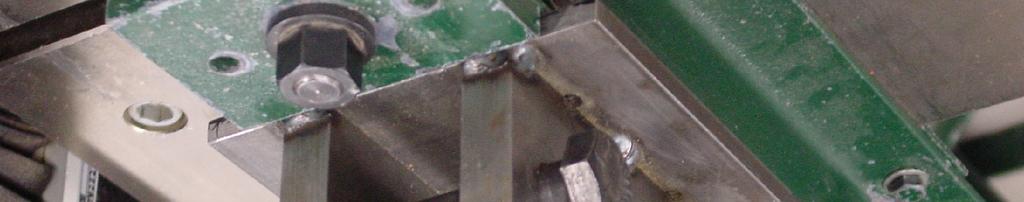
75 Figure 3.1: Three-point bolt bending test set-up. Figure 3.11: Cantilever bolt bending test set-up. 42

76 Moisture Content Tests Moisture content tests were performed in accordance with ASTM D Standard Test Method for Direct Moisture Content Measurement of Wood and Wood- Based Materials (ASTM, 24). Specimens were obtained from previously tested dowel embedment specimens, which had been returned to the conditioning chamber following testing to ensure equilibration. Method B for oven drying was the desirable method for determining the moisture content for each specimen. Specimens were placed in an oven at a temperature of approximately 12 ºC (215 ºF) until mass had stabilized as determined by intermediate measurements. Moisture content was calculated as follows: MC% = (A-B)/B * 1 (3.1) A = Original mass (g). B = Oven-dry mass (g) Specific Gravity Tests Specific gravity tests were performed in accordance with ASTM D Standard Test Methods for Specific Gravity of Wood and Wood-Based Products (ASTM, 24). Specimens tested were previously used to determine moisture content, providing specific gravity (SG) results for oven-dry volume. Method B for determining volume by water immersion was chosen for precision considering the irregular surface of the specimens. Specific gravity was calculated as follows: SG = W/V (3.2) W = Weight of specimen at approximately 12% moisture content. V = Oven-dry volume of specimen at approximately 12% moisture content. 43

77 3.8 - Test Data Analysis Strength and serviceability parameters of full-connection cyclic testing were obtained based on the Proposed Test Method for Dynamic Properties of Connections Assembled with Mechanical Fasteners (Dolan, 1994). Primary parameters included connection capacity, equivalent elastic-plastic (E.E.P.) yield load, and ductility. To evaluate the above parameters, the maximum load and corresponding displacement for each successive hysteretic loop were used to create an envelope curve similar to that of a monotonic test. The parameters and points of interest used to determine the desired connection characteristics are illustrated in Figure 3.12 and defined below. E.E.P Yield Load E.E.P. Yield Displacement Connection Capacity E.E.P. Failure Displacement Envelope curve 4% Max Load Figure 3.12: Bi-linear and envelope curves shown on a typical specimen. A bi-linear curve was produced for each specimen to evaluate parameters of interest. An initial diagonal region originating at the point on the horizontal axis where slack in the 44

78 connection had been taken up passes through the point on the envelope curve corresponding to 4% of the maximum load. The horizontal region representing equivalent elastic-plastic (E.E.P.) yield load intersected the initial diagonal line, and extended until failure displacement. Failure displacement was the displacement corresponding to failure, which occurred at 8% of ultimate capacity. The E.E.P. yield load, by definition, falls between the maximum load and 8% of the maximum load, and was defined such that the area under the bi-linear curve was equal to the area under the envelope curve up to failure displacement. Ductility ( ) was then defined as failure/ yield. Strain energy, hysteretic energy, equivalent viscous damping, and cyclic stiffness are all determined on a cycle-by-cycle basis for each tested specimen. Definitions are provided below and illustrated in Figure The strain energy for a given cycle was defined as the sum of the areas enclosed by the triangles CJK and REK. Hysteretic energy for a given cycle was defined as the sum of the areas enclosed by the load-deflection curve (the shaded portion on Figure 3.13). Cyclic stiffness for a given cycle was defined as the slope of the line EJ. The equivalent viscous damping ratio ( for a given cycle is defined as hysteretic energy/2 *strain energy. Figure 3.13: Hysteretic energy and strain energy. 45

79 When evaluating the energy-based parameters on a cycle-by-cycle basis, it was necessary to address the previously noted errors occurring within the protocol. When analyzing the data, it was not possible to strictly adhere to the prescribed protocol due to the potential addition or exclusion of half cycles. When a half cycle was erroneously added to the protocol, it was excluded in data analysis, and the following primary cycle experienced reversal in the direction of initiation. When a half cycle was erroneously excluded from the protocol, the previous half cycle was multiplied by two to account for the total energy of the cycle, and the following primary cycle experienced the same phenomenon as before. Refer to Figure 3.14 for an example time-displacement plot of the erroneous half cycles. Exclusion of Half-Cycle Displacement Additional Half-Cycle Time Figure 3.14: Time-displacement plot with erroneous half cycles. 46

80 Results and Discussion General The present study is comprised of two hundred single and multiple-bolt connection tests subjected to reverse cyclic loading. Bolt diameter, member dimensions, joint geometry, and row spacing were varied to produce desired connection yield modes. This chapter provides cyclic test results. Typical load-displacement plots for each series are presented in this chapter, and full results are available in Appendix A. Results of connection performance characteristics including connection capacity, 5% offset yield, equivalent elastic plastic yield, elastic stiffness, displacement at failure, and ductility ratio are listed for each configuration. Values for each series were divided by the number of bolts in the connection and then compared with the mean value for the single-bolt series. The ratio developed is analogous to the group action factor, with a value of 1. assigned to single-bolt connection means. This comparison was made for the 5% offset yield strength and connection capacity and will be referred to as the normalized value throughout this discussion. A similar approach was taken for connection ductility ratio; however the value was not divided by the number of bolts in the connection. The 5% offset yield and capacity values from testing were compared with values predicted using the Yield Model (YM). The YM does not, however, account for brittle failure mechanisms such as splitting, net-section tension rupture, and group tear-out. The capacity and failure mode from tested specimens were compared to those determined using Appendix E of the 21 NDS (AF&PA, 21). Appendix E provides capacities and failure modes based on the local stresses in the wood member being considered. 47

81 Statistical analyses were performed to make inferences regarding the relative effects of row spacing on connection ductility ratio, connection capacity, and 5% offset yield strength, and to determine the ability of the YM to accurately predict the 5% offset yield strength and capacity of bolted connections subjected to the prescribed cyclic loading. It was assumed that the data was normally distributed, and the mean and population variances were equal. Two-sample t-tests, with a significance level of =.5, were performed to test the null hypothesis that any two population means are equal. Values for the t-statistic were generated based on equation 4.1 and compared with t- critical values obtained from an elementary statistics tables (Johnson, 1976) based on, and number of degrees of freedom. It was assumed that a normal data distribution as chosen for analysis would be sufficiently accurate based on sample size, and that alternative methods of data distribution would likely have yielded similar results. x t statistic s / n (4.1) where: x = Sample mean. = Population mean. s n = Sample standard deviation. = Square root of sample size. Throughout this discussion, I will refer to failures modes either as ductile or brittle. These failure modes, or mechanisms as often referred to, are subjectively assigned based primarily on test observations and their subsequent load-displacement 48

82 plots. Tests experiencing ductile failure mechanisms typically exhibited relatively large displacements prior to failure. Furthermore, failure was characterized by a gradual loss of strength following maximum load. Conversely, a brittle failure was characterized by a sudden catastrophic failure such as splitting, group tear-out or tension failures in which the load resisted as displacement increased was significantly below the connection s maximum load Mode II Yield Connections expected to display Yield Mode II were fabricated using two-inch thick nominal lumber for both members, with 19.1 mm (¾ in.) diameter bolts. The width of the members was varied to accommodate the number of rows and row spacing. Additional information regarding specific configurations may be found in Table Cyclic Test Results Single row configurations consisting of single-bolt and three-bolt arrangements were subjected to a displacement controlled cyclic protocol as described in Chapter 3. The reference deformation was equal to 11.4 mm (.45 in.) for single-bolt tests, and 1.7 mm (.42 in.) for three-bolt tests. All bolts remained straight and pivoted about the member interface, consistent with Mode II yield behavior. The primary mode of failure observed was splitting through the centerline of the bolt row, however, a combination of splitting on the compression stroke and plug shear on the tension stroke was also observed as illustrated in Figure 4.1. A typical load-deflection plot for the single-row configuration is shown in Figure

83 Figure 4.1: Photograph of Mode II splitting/plug shear failure Figure 4.2: Typical load-deflection plot. Mode II yield; single bolt. 5

84 Three rows of one bolt-per-row arrangements consisting of 2D and 3D row spacings were subjected to a displacement controlled cyclic protocol as described in Chapter 3. The reference deformation was equal to 1.2 mm (.4 in.) for both sets. All bolts remained straight and pivoted about the member interface, consistent with Mode II yield behavior. There was an even distribution of group tear-out and splitting failures with the 2D spacing, while splitting through the centerline of the bolt rows was the dominant mode of failure with the 3D spacing. Splitting failures usually featured either splitting of all three rows of one member, or splitting of one row of a member and the opposite rows in the other member. Figure 4.3 illustrates splitting through the centerline of the outer two bolt rows of the main member, and center bolt row of the side member. A typical load-deflection plot for the above configurations is shown in Figure 4.4. Figure 4.3: Photograph of different types of row splitting for a single specimen. Mode II yield; three rows of one bolt. 51

85 Figure 4.4: Typical load-deflection plot. Mode II yield; three rows of one bolt. Three rows of three bolts-per-row arrangements consisting of 2D, 2.5D, and 3D row spacings were subjected to a displacement controlled cyclic protocol as described in Chapter 3. The reference deformation was equal to 8.9 mm (.35 in.) for all three sets. All bolts remained straight and pivoted about the member interface, consistent with Mode II yield behavior. There was an even distribution of group tear-out and splitting through the centerline of the bolt row failures with the 2D spacing, and a relatively even distribution of splitting through the centerline and group tear-out failures seen in the 2.5D and 3D spacing. Typically, the splitting failures occurred in the same manner as described for three rows of one bolt-per-row splitting failures. An example of group tearout failure is shown in Figure 4.5. A typical load-deflection plot for the three rows of three configurations is shown in Figure

86 Figure 4.5: Photograph of group tear-out. Mode II yield; three rows of three bolts Figure 4.6: Typical load-deflection plot. Mode II yield; three rows of three bolts. 53

87 Connection performance results and material properties are displayed in Tables 4.1 and 4.2 respectively. Results were based on ten replications per configuration, unless otherwise noted. Configurations predicted to display Mode II yield generally displayed brittle failure modes occurring at displacement levels near or just above capacity. As row spacing increased from 2D to 3D, the mode of failure progressed towards splitting through the centerline of the bolt row rather than by group tear-out or net-section tension rupture. This trend was likely due to the decreased local stresses in the wood between rows of bolts. 54

88 Table 4.1a: Average connection performance results for Mode II yield predictions (SI). C21(1R1) C22(1R3) C24(3R1 2D) C25(3R1 3D) Mean COV (%) Mean Max Load (N) (mm) COV (%) Mean COV (%) Mean Load/Bolt (N) Failure Load (N) (mm) Load/Bolt (N) % Max (N) (mm) E.E.P. Yield (N)* (mm) Load/Bolt (N) % Offset Yield (N) (mm) Load/Bolt (N) Elastic Stiff. (N/mm) E.E.P. Energy (N*m)** Ductility Ratio COV (%) C28(3R3 2D) C3(3R3 2.5D) C29(3R3 3D) Mean COV (%) Mean COV (%) Mean COV (%) Max Load (N) (mm) Load/Bolt (N) Failure Load (N) (mm) Load/Bolt (N) % Max (N) (mm) E.E.P. Yield (N)* (mm) Load/Bolt (N) % Offset Yield (N) (mm) Load/Bolt (N) Elastic Stiff. (N/mm) E.E.P. Energy (N*m)** Ductility Ratio *E.E.P. Yield: Equivalent Elastic-Plastic Yield **E.E.P. Energy: Equivalent Elastic-Plastic Energy 55

89 Table 4.1b: Average connection performance results for Mode II yield predictions (Std.). C21(1R1) C22(1R3) C24(3R1 2D) C25(3R1 3D) Mean COV (%) Mean Max (in) COV (%) Mean Load/Bolt (lbs) Failure (in) Load/Bolt (lbs) % Max (lbs) COV (in) E.E.P. Yield (lbs)* (in) Load/Bolt (lbs) % Offset Yield (lbs) (in) Load/Bolt (lbs) Elastic Stiff. (lb/in) E.E.P. Energy (lb*in)** Ductility Ratio Mean COV (%) C28(3R3 2D) C3(3R3 2.5D) C29(3R3 3D) Mean COV (%) Mean COV (%) Mean Max COV (in) Load/Bolt (lbs) Failure (in) Load/Bolt (lbs) % Max (lbs) (in) E.E.P. Yield (lbs)* (in) Load/Bolt (lbs) % Offset Yield (lbs) (in) Load/Bolt (lbs) Elastic Stiff. (lb/in) E.E.P. Energy (lb*in)** Ductility Ratio *E.E.P. Yield: Equivalent Elastic-Plastic Yield **E.E.P. Energy: Equivalent Elastic-Plastic Energy 56

90 Table 4.2a: Average connection material properties for Mode II yield predictions (SI). C21(1R1) C22(1R3) C24(3R1 2D) C25(3R1 3D) Main Member Mean COV (%) Mean COV (%) Mean COV (%) Mean COV (%) M.C. (%) S.G D.E. 5% Offset Yield (N) D.E. Capacity (N) Side Member Mean COV (%) Mean COV (%) Mean COV (%) Mean COV (%) M.C. (%) S.G D.E. 5% Offset Yield (N) D.E. Capacity (N) C28(3R3 2D) C3(3R3 2.5D) C29(3R3 3D) Main Member Mean COV (%) Mean COV (%) Mean COV (%) M.C. (%) S.G D.E. 5% Offset Yield (N) D.E. Capacity (N) Side Member Mean COV (%) Mean COV (%) Mean COV (%) M.C. (%) S.G D.E. 5% Offset Yield (N) D.E. Capacity (N) M.C.: Moisture Content S.G.: Specific Gravity D.E.: Dowel Embedment Data xxd: Refers to Row Spacing 57

91 Table 4.2b: Average connection material properties for Mode II yield predictions (Std.). C21(1R1) C22(1R3) C24(3R1 2D) C25(3R1 3D) Main Member Mean COV (%) Mean COV (%) Mean COV (%) Mean COV (%) M.C. (%) S.G D.E. 5% Offset Yield (lbs) D.E. Capacity (lbs) Side Member Mean COV (%) Mean COV (%) Mean COV (%) Mean COV (%) M.C. (%) S.G D.E. 5% Offset Yield (lbs) D.E. Capacity (lbs) C28(3R3 2D) C3(3R3 2.5D) C29(3R3 3D) Main Member Mean COV (%) Mean COV (%) Mean COV (%) M.C. (%) S.G D.E. 5% Offset Yield (lbs) D.E. Capacity (lbs) Side Member Mean COV (%) Mean COV (%) Mean COV (%) M.C. (%) S.G D.E. 5% Offset Yield (lbs) D.E. Capacity (lbs) M.C.: Moisture Content S.G.: Specific Gravity D.E.: Dowel Embedment Data xxd: Refers to Row Spacing 58

92 4.3 - Mode III s Yield Connections expected to display Yield Mode III s were fabricated using 12 mm (4 in.) thick nominal lumber for the main member, and 51 mm (2 in.) thick nominal lumber for the side member, using 12.7 mm (½ in.) diameter bolts. The nominal member width for single-row configurations was 12 mm (4 in.), and 152 mm (6 in.) for the remaining configurations. Additional information regarding specific configurations can be found in Table Cyclic Test Results Single-row configurations consisting of one-bolt and three-bolt arrangements were subjected to a displacement controlled cyclic protocol as described in Chapter 3. The reference deformation was equal to 13.5 mm (.53 in.) for single-bolt tests, and 11.4 mm (.45 in.) for three-bolt tests. All bolts in the single-bolt configuration tests formed a clearly defined plastic hinge, consistent with Mode III s yield behavior. The single-row, three-bolt configurations often displayed a mixed mode yield mechanism, meaning that the bolts within a given test specimen may not all achieve the same yield mode. This is due to unequal load distribution to bolts in a connection as well as material property variations. The yield modes observed were Mode III s, and a mixed yield mode ranging from Mode II to Mode III s. When Mode III s was observed, the plastic hinge formation was only slight, yet still evident. The primary mode of failure observed was splitting through the centerline of the bolt row. However, a combination of splitting and plug shear was also observed. Typical splitting failures for the single-bolt row and loaddeflection plot for the single-bolt configuration are shown in Figures 4.7 and

93 Figure 4.7: Photograph of typical splitting failure. Mode III s yield; one row of three bolts Figure 4.8: Typical load-deflection plot. Mode III s yield; single bolt. 6

94 Three rows of one bolt-per-row arrangements consisting of 2D, 2.5D and 3D row spacings were subjected to a displacement controlled cyclic protocol as described in Chapter 3. The reference deformation was equal to 11.4 mm (.45 in.) for all three sets. The yield modes observed were Mode III s, Mode IV, and a mixed yield mode ranging from Mode III s to Mode IV. When Mode III s was observed, the formation of a plastic hinge was very distinct. However, when Mode IV yield was present, the reverse bending caused by the formation of two plastic hinges in the bolt was only very slight. As row spacing was increased, the primary mode of failure observed was splitting through the centerline of the bolt row, or splitting with plug shear on the opposite stroke. However, group tear-out failures were also observed. An example of splitting failure is shown in Figure 4.9. A typical load-deflection plot for a three rows of one bolt-per-row configuration is shown in Figure 4.1. Reverse bending, as referenced above and in future discussions, refers to the geometry of the bolt after it has yielded. Two plastic hinges form by definition, inducing two bend angles in the bolt. If the bend angles are equal and opposite such that bolt ends are parallel, then reverse bending is present. If two plastic hinges form, but the bolt ends are not parallel, then reverse bending is not present. 61

95 Figure 4.9: Photograph of typical splitting. Mode III s yield; three rows of one bolt Figure 4.1: Typical load-deflection plot. Mode III s yield; three rows of one bolt. 62

96 Three rows of three bolts-per-row arrangements consisting of 2D and 3D row spacings were subjected to a displacement controlled cyclic protocol as described in Chapter 3. The reference deformation was equal to 7.6 mm (.3 in.) for both sets. The yield modes observed were Mode III s, and a mixed yield mode ranging from Mode II to Mode III s. When Mode III s was observed, the formation of a plastic hinge was typically very slight, yet still evident depending on the magnitude of load that a given row of bolts had resisted prior to failure. The primary mode of failure observed in connections with 2D row spacing was group tear-out, while splitting through the centerline of the bolt row was typical for connections with 3D row spacing. An example of group tear-out failure is shown in Figure A typical load-deflection plot for the three rows of three bolts-perrow configuration is shown in Figure 4.12 Figure 4.11: Photograph of group tear-out. Mode III s yield, three rows of three bolts. 63

97 Figure 4.12: Typical load-deflection plot. Mode III s yield, three rows of three bolts. Connection performance results and material properties are displayed in Tables 4.3 and 4.4 respectively. Results are based on ten replications per configuration, unless otherwise noted. Generally, poor agreement was found between experimental results and the predictions of the Yield Model; however single-bolt connections were accurately predicted by the model. Connections with three rows of one bolt always attained or surpassed the yield mode predicted by the YM, while connections with three bolts-perrow did not always achieve the predicted yield mode. Splitting through the centerline of the row of bolts was the ultimate failure mode for the majority of these tests. However, configurations using one bolt-per-row displayed signs of bearing failure at larger displacements prior to splitting. Inaccuracies of the YM for these configurations will be discussed in detail near the end of this chapter 64

98 Table 4.3a: Average connection performance results for Mode III s yield predictions (SI). C11(1R1) C12(1R3) C14(3R1 2D) C16(3R1 2.5D) Mean COV (%) Mean Max Load (N) (mm) COV (%) Mean COV (%) Mean Load/Bolt (N) Failure Load (N) (mm) Load/Bolt (N) % Max (N) (mm) E.E.P. Yield (N)* (mm) Load/Bolt (N) % Offset Yield (N) (mm) Load/Bolt (N) Elastic Stiff. (N/mm) E.E.P. Energy (N*m)** Ductility Ratio COV (%) C15(3R1 3D) C18(3R3 2D) C19(3R3 3D) Mean COV (%) Mean COV (%) Mean COV (%) Max Load (N) (mm) Load/Bolt (N) Failure Load (N) (mm) Load/Bolt (N) % Max (N) (mm) E.E.P. Yield (N)* (mm) Load/Bolt (N) % Offset Yield (N) (mm) Load/Bolt (N) Elastic Stiff. (N/mm) E.E.P. Energy (N*m)** Ductility Ratio *E.E.P. Yield: Equivalent Elastic-Plastic Yield **E.E.P. Energy: Equivalent Elastic-Plastic Energy 65

99 Table 4.3b: Average connection performance results for Mode III s yield predictions (Std.) C11(1R1) C12(1R3) C14(3R1 2D) C16(3R1 2.5D) Mean COV (%) Mean Max (in) COV (%) Mean Load/Bolt (lbs) Failure (in) Load/Bolt (lbs) % Max (lbs) (in) E.E.P. Yield (lbs)* (in) Load/Bolt (lbs) % Offset Yield (lbs) (in) Load/Bolt (lbs) Elastic Stiff. (lb/in) E.E.P. Energy (lb*in)** Ductility Ratio COV (%) Mean COV (%) C15(3R1 3D) C18(3R3 2D) C19(3R3 3D) Mean COV (%) Mean COV (%) Mean COV (%) Max (in) Load/Bolt (lbs) Failure (in) Load/Bolt (lbs) % Max (lbs) (in) E.E.P. Yield (lbs)* (in) Load/Bolt (lbs) % Offset Yield (lbs) (in) Load/Bolt (lbs) Elastic Stiff. (lb/in) E.E.P. Energy (lb*in)** Ductility Ratio *E.E.P. Yield: Equivalent Elastic-Plastic Yield **E.E.P. Energy: Equivalent Elastic-Plastic Energy 66

100 Table 4.4a: Average connection material properties for Mode III s yield predictions (SI). C11(1R1) C12(1R3) C14(3R1 2D) C16(3R1 2.5D) Main Member Mean COV (%) Mean COV (%) Mean COV (%) Mean COV (%) M.C. (%) S.G D.E. 5% Offset Yield (N) D.E. Capacity (N) Side Member Mean COV (%) Mean COV (%) Mean COV (%) Mean COV (%) M.C. (%) S.G D.E. 5% Offset Yield (N) D.E. Capacity (N) C15(3R1 3D) C18(3R3 2D) C19(3R3 3D) Main Member Mean COV (%) Mean COV (%) Mean COV (%) M.C. (%) S.G D.E. 5% Offset Yield (N) D.E. Capacity (N) Side Member Mean COV (%) Mean COV (%) Mean COV (%) M.C. (%) S.G D.E. 5% Offset Yield (N) D.E. Capacity (N) M.C.: Moisture Content S.G.: Specific Gravity D.E.: Dowel Embedment Data xxd: Refers to Row Spacing 67

101 Table 4.4b: Average connection material properties for Mode III s yield predictions (Std.). C11(1R1) C12(1R3) C14(3R1 2D) C16(3R1 2.5D) Main Member Mean COV (%) Mean COV (%) Mean COV (%) Mean COV (%) M.C. (%) S.G D.E. 5% Offset Yield (lbs) D.E. Capacity (lbs) Side Member Mean COV (%) Mean COV (%) Mean COV (%) Mean COV (%) M.C. (%) S.G D.E. 5% Offset Yield (lbs) D.E. Capacity (lbs) C15(3R1 3D) C18(3R3 2D) C19(3R3 3D) Main Member Mean COV (%) Mean COV (%) Mean COV (%) M.C. (%) S.G D.E. 5% Offset Yield (lbs) D.E. Capacity (lbs) Side Member Mean COV (%) Mean COV (%) Mean COV (%) M.C. (%) S.G D.E. 5% Offset Yield (lbs) D.E. Capacity (lbs) M.C.: Moisture Content S.G.: Specific Gravity D.E.: Dowel Embedment Data xxd: Refers to Row Spacing 68

102 4.4 - Mode IV Yield Connections expected to display Yield Mode IV were fabricated using 12 mm (4 in.) thick by 12 mm (4 in.) thick nominal lumber for both members, with 6.4 mm (¼ in.) diameter bolts. Additional information regarding specific configurations can be found in Table Cyclic Test Results Single-row configurations consisting of one-bolt and three-bolt arrangements were subjected to a displacement controlled cyclic protocol as described in Chapter 3. The reference deformation was equal to 2.3 mm (.8 in.) for single-bolt tests, and 15.5 mm (.61 in.) for three-bolt tests. All bolts in the single-bolt configuration formed two clearly defined plastic hinges and exhibited reverse bending consistent with Mode IV. Bolts in the single-row of three bolts configuration displayed either Yield Mode IV, or a mixed mode yield ranging from Mode III s to Mode IV for each specimen. Bolts exhibiting Mode III s yield typically formed two plastic hinges, however, reverse bending was not present. The primary failure mode observed in single-bolt tests was bolt fatigue, while splitting through the centerline of the bolt row was the failure mode observed in the single-row of three bolts configuration. Of the bolts that did not fracture, minor to significant necking, or reduction in cross-sectional area due to bolt fatigue, was observed at plastic hinge locations. A splitting failure showing necking of the bolt, and a loaddeflection plot indicating ductile failure are shown in Figures 4.13 and 4.14 respectively. 69

103 Necking Figure 4.13: Photograph of necking. Mode IV yield; single bolt Figure 4.14: Typical load-deflection plot. Mode IV Yield; single bolt. 7

104 Three rows of one bolt-per-row arrangements consisting of 2D and 3D row spacing were subjected to a displacement controlled cyclic protocol as described in Chapter 3. The reference deformation was equal to 15.5 mm (.61 in.) for both sets. All bolts in this series exhibited Mode IV yield prior to failure. Even distributions of splitting and bolt fatigue failure mechanisms were observed in the 2D row spacing configuration. For the configuration with 3D spacing, bolt fatigue was the predominant failure mechanism. Bolt fatigue failure is shown in Figure 4.15, and a typical load-deflection plot for the three rows of one bolt configuration is shown in Figure Figure 4.15: Photograph of bolt failure. Mode IV yield; three rows of one bolt. 71

105 Figure 4.16: Typical load-deflection plot. Mode IV yield; three rows of one bolt. Three rows of three bolts-per-row arrangements consisting of 2D and 3D row spacings were subjected to a displacement controlled cyclic protocol as described in Chapter 3. The reference deformation was equal to 15.5 mm (.61 in.) for both sets. These configurations displayed either Yield Mode IV, or a mixed mode yield ranging from Mode III s to Mode IV. Bolts exhibiting Mode III s yield typically formed two plastic hinges, however, reverse bending was not present. For the configuration with 2D row spacing, wood splitting through the centerline of the bolt row(s) was the predominant failure mechanism. Wood splitting through the centerline of the bolt row(s) was also the predominant failure mechanism when row spacing was 3D, however, two bolt fatigue failures were observed, implicating a slightly larger degree of ductility than exhibited in the 2D row spacing configuration. A splitting failure through the centerline of the bolt row(s) is shown in Figure 4.17, and a typical load-deflection plot indicating ductile failure is shown in Figure

106 Figure 4.17: Photograph of spitting. Mode IV yield; three rows of three bolts Figure 4.18: Typical load-deflection plot. Mode IV yield; three rows of three bolts. 73