Course Outline MODEL INFORMATION. Bayes Decision Theory. Unsupervised Learning. Supervised Learning. Parametric Approach. Nonparametric Approach

Transcription

1 Course Outline MODEL INFORMATION COMPLETE INCOMPLETE Bayes Decision Theory Supervised Learning Unsupervised Learning Parametric Approach Nonparametric Approach Parametric Approach Nonparametric Approach Optimal Rules Plug-in Rules Density Estimation Geometric Rules (K-NN, MLP) Mixture Resolving Cluster Analysis (Hard, Fuzzy)

2 Two-dimensional Feature Space Supervised Learning

3 Chapter 3: Maximum-Likelihood & Bayesian Parameter Estimation Introduction Maximum-Likelihood Estimation Bayesian Estimation Curse of Dimensionality Component analysis & Discriminants

4 Bayesian framework To design an optimal classifier we need: 3 P(w i ) : priors P(x w i ) : class-conditional densities What if this information is not available? Supervised Learning: Design a classifier based on a set of labeled training samples Assume priors are known Sufficient no. of training samples available to estimate P(x w i ) Pattern Classification, Chapter 3

5 Assumption: Parametric model of P(x w i ) is available 4 For example, for Gaussian pdf assume P(x w i ) ~ N( µ i, S i ), i =,..,c Parameters (µ i, S i ) are not known, but labeled training samples are available to estimate them Parameter estimation Maximum-Likelihood (ML) estimation Bayesian estimation For large n, estimates from the two methods are nearly identical Pattern Classification, Chapter 3

6 5 ML parameter estimation (MLE): Parameters are assumed to be fixed but unknown! Best parametric estimates are obtained by maximizing the probability of obtaining the samples observed Bayesian parameter estimation: Unknown parameters are random variables with some known prior distribution; Use prior and samples to obtain the posteriori density Parameter estimate is derived from posteriori & loss fn. Both methods use P(w i x) for decision rule! Pattern Classification, Chapter 3

7 Maximum-Likelihood Parameter Estimation Has good convergence properties as the sample size increases; estimated parameter value approaches the true value as n increases Most simple method for parameter estimation General principle Assume we have c classes and P(x w j ) ~ N( µ j, S j ) P(x w j ) º P (x w j, q j ), where 6 q = ( µ j, S j ) = ( µ j, µ j,..., s j, s j,cov(x m j,x n j )...) Use class w j samples to estimate class w j parameters: µ j, S j Pattern Classification, Chapter 3

8 Use the training samples to estimate q q = (q, q,, q c ); 7 q i (i =,,, c) is parameter for the w i Sample set D contains n iid samples, x, x,, x n P(D P(D q) = k= n ÕP(x k= k q) = F( q) q) is called the likelihood of q w.r.t. the set of samples) ML estimate of q is the value that maximizes P(D q) It is the value of q that best agrees with the observed training samples qˆ Pattern Classification, Chapter 3

9 8 Pattern Classification, Chapter 3

10 ML estimation Let q = (q, q,, q p ) t and Ñ q be the gradient operator 9 Ñ q = é ê ë q ù,,..., ú q q û p t We define l(q) as the log-likelihood function l(q) = ln P(D q) Determine q that maximizes the log-likelihood qˆ = argmaxl( q) q Pattern Classification, Chapter 3

11 0 Set of necessary conditions for an optimum: k= n ( Ñql = å Ñq lnp(xk k= q)) Ñ q l = 0 Pattern Classification, Chapter 3

12 P(x µ) ~ N(µ, S); µ is not known but S is known Samples are drawn from a multivariate Gaussian lnp(x k µ ) = - ln ( [ d p) S ] - (x k - µ ) t - å(x k - µ ) and Ñ qµ lnp(x k µ ) = - å(x k - µ ) The ML estimate for µ must satisfy: k= n å S k= - ( x k - µ ˆ ) = 0 Pattern Classification, Chapter 3

13 Multiplying by S and rearranging terms: µ ˆ = n k= n å x k k= MLE of the mean of the Gaussian distribution is the sample mean Conclusion: Given P(x k w j, q j ), j =,,,c to be Gaussian in d- dimensions, estimate the vector q = (q, q,, q c ) t and then use the maximum a posteriori rule (Bayes decision rule) Pattern Classification, Chapter 3

14 3 ML Estimation: Univariate Gaussian Case: unknown µ & s q = (q, q ) = (µ, s ) For the kth sample (observation) l = lnp(x k q) = æ s ç (lnp(x ç sq Ñql = ç s ç (lnp(x è sq ì ï (xk - q) = 0 q í ï (xk - q) - + ï î q q - lnpq k k ö q)) q)) ø = 0 = - q 0 (x k - q ) Pattern Classification, Chapter 3

15 Pattern Classification, Chapter 3 4 Introduce summation to account for n samples: Combining () and (), we get: n ) (x ; n x n k k k n k k k å µ - = s å = µ = = = = ï ï î ï ï í ì å å = q - q + q - å = - q q = = = = = = n k k n k k k n k k k () 0 ˆ ) ˆ (x ˆ () 0 ) (x ˆ

16 5 ML estimate for s is biased é E êë n S(x n - n i - x) =. An unbiased estimator for S is: ù úû s ¹ s k= n t C = å (xk - µ )(xk - µ ˆ ) $! n!!!! - k= #!!!!!" Sample covariancematrix Pattern Classification, Chapter 3

17 ML vs. Bayesian Parameter Estimation Unknown Parameter is the Prob. of Heads of a coin

18

19

20

21

22 Bayesian Estimation (Bayesian learning) In MLE q was supposed to have a fixed value In Bayesian learning q is a random variable Direct estimation of posterior probabilities P(w i x) lies at the heart of Bayesian classification Goal: compute P(w i x, D) Given the training sample set D, Bayes formula can be written P( w i x, D ) = c P(x w åp(x w j= i, D ).P( w j i, D ).P( w D ) j D ) Pattern Classification, Chapter 3

23 Derivation of the preceding equation: P(x, D w P(x D ) P( w i ) = Thus : P( w P( w i i = ) = P(x Dw åp(x, w j i D ) (Training sample provides this!) x, D ) = j D ) P(x c j= i ).P( D w w åp(x w i, D j i i ) ).P( w i, D ).P( w ) j ) Pattern Classification, Chapter 3

24 Bayesian Parameter Estimation: Gaussian Case 3 Goal: Estimate q using the a-posteriori density P(q D) The univariate Gaussian case: P(µ D) µ is the only unknown parameter P(x µ ) ~ N( µ, s P( µ ) ~ N( µ 0, s 0 ) ) µ 0 and s 0 are known! Pattern Classification, Chapter 4

25 P( µ D ) = = P( D µ ).P( µ ) ò P( D µ ).P( µ )dµ k= n a Õ P(x µ ).P( µ k= Reproducing density k ) () 4 P( µ D ) ~ N( µ n, s n ) () The updated parameters of the prior: µ n = and æ ç èn s n 0 ns s = 0 0 s ns + s 0 0 s ö µ ˆ ø + s n + ns s 0 + s. µ 0 Pattern Classification, Chapter 4

26 5 Pattern Classification, Chapter 4

27 The univariate case P(x D) P(µ D) has been computed P(x D) remains to be computed! 6 P (x D) = ò P(x µ ).P( µ D)dµ is Gaussian It provides: P(x D ) ~ N( µ n, s + s n ) Desired class-conditional density P(x D j, w j ) P(x D j, w j ) together with P(w j ) and using Bayes formula, we obtain the Bayesian classification rule: Max wj [ P( w x, D ] º Max[ P(x w, D ).P( w )] j wj j j j Pattern Classification, Chapter 4

28 Bayesian Parameter Estimation: General Theory 7 P(x D) computation can be applied to any situation in which the unknown density can be parametrized: the basic assumptions are: The form of P(x q) is assumed known, but the value of q is not known exactly Our knowledge about q is assumed to be contained in a known prior density P(q) The rest of our knowledge about q is contained in a set D of n random variables x, x,, x n drawn from P(x) Pattern Classification, Chapter 5

29 The basic problem is:. Compute the posterior density P(q D). Derive P(x D) Using Bayes formula, we have: 8 P( D q).p( q) P( q D ) = òp( D q).p( q)dq And by independence assumption:, P( D q) = k= n Õ k= P(x k q) Pattern Classification, Chapter 5

30 Iris Dataset Three types of iris flower: Setosa, Versicolor, Virginica Four features: Sepal length, sepal width, petal length petal width (all in cm.) 50 patterns/class Available in UCI Machine Learning Repository Fisher, R. A. "The use of multiple measurements in taxonomic problems" Annual Eugenics, 7, Part II, (936)

31 PCA Explained variance ratio st component 0.95 nd component 0.053

32 LDA Explained variance ratio st component 0.99 nd component 0.009

33 ISOMAP

34 Low Dimensional Embedding of High Dimensional Data Given n patterns in a d-dim space, embed the points in m dimensions, m<<d Purpose: data compression; avoid overfitting by reducing dimensionality; find meaningful low-dim structures in their high-dimensional observations Feature selection v. feature extraction Feature extraction: linear v. non-linear Linear feature extraction or projection: unsupervised (PCA) v. supervised (LDA) Non-linear feature extraction (Isompap)

35 Eigen Decomposition Given a linear transformation A, a non-zero vector w is an eigenvector of A if it satisfies the eigenvalue equation for some scalar l Aw = lw Ex. é ù ê ú ë û Solution: Aw - liw = 0 Eigenvalue: Eigenvector: Þ( A- li) w = 0 Þdet( A- li) = 0 é- l ù det ê = 0 - l ú ë û ( -l) - = 0 l - 4l+ 3= 0 Þ l = andl = 3 é- l ùée ù ê 0 l úê ú = ë - ûëe û é- l ùée ù ê 0 l úê ú = ë - ûëe û (Characteristic equation) Eigenvector is normalized as e + e = ée ù é- ù ê ú = ê e ú ë û ë û ée ù é ù ê ú = ê e ú ë û ë û e e

36 y μ = [, ] é5 ù Σ = ê 3 ú ë û x Eigenvectors: Eigenvalues: é ù ê ú ë û é ù ê ú ë û

37 μ = [4,, ] é 0 0ù Σ = ê 0 0 ú ê ú êë0 0 úû é ù ê Eigenvectors: ú ê ú êë úû é ù Eigenvalues: ê ú ê ú êë úû

38 PCA Y = w T X Find a transformation w, such that the w T x is dispersed the most (maximum distribution)

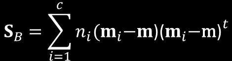
39 Scatter Matrices m = mean vector of all n patterns (grand mean) mi = mean vector of class i patterns S W = within-class scatter matrix. It is proportional to the sample covariance matrix for the pooled d- dimensional data. It is symmetric and positive semidefinite, and is usually nonsingular if n > d S B = between-class scatter matrix. It is symmetric and positive semidefinite, but because it is the outer product of two vectors, its rank is at most (C-) S T = total scatter of all n patterns For any w, S B w is in the direction of (m -m )

40 (9) (97) (09) (5) (3) (6)

41 Principal Component Analysis (PCA) What is the best representation of n d-dim samples x,,x n by a single point x 0? Find x 0 such that the sum of the squared distances between x 0 and all x k is minimized Define squared-error criterion function J 0 (x 0 ) by n ( x ) = å x -x 0 0 k k = and find x 0 that minimizes J 0. J o The solution is given by x 0 =m, where m is the sample mean, n m= åxk. n k =,

42 Principal Component Analysis Sample mean is a zero-dim representation of data; It does not reveal any of the data variability What is the best one-dim representation? Project data to a line through the sample mean. If e is a unit vector in the direction of the line, equation of the line can be written as x= m+ae, Representing x k by m+a k e, find the optimal set of coefficients a k by minimizing the squared error n n n e = åp m+ ke - xk P = åp ke- xk -m P k= k= J ( a,..., a, ) ( a ) a ( ) n n n t åak PeP åake xk m åpxk m P k= k= k= = - ( - ) + ( - ).

43 Principal Component Analysis Since e = differentiate with respect to a k, and set the derivative to zero t a = e ( x -m). k To obtain a least-squares solution, project the vectors x k to the line in the direction of e that passes through the sample mean What is the best direction e for the line? The solution involves the scatter matrix S n t S= å( xk -m)( xk -m). k = The best direction is the eigenvector of the scatter matrix with the largest eigenvalue k

44 Principal Component Analysis Scatter matrix S T is real and symmetric; it s eigenvectors are orthogonal and form a set of basis vectors for representing any vector x The coefficients a i in Eq. (89) are the components of x in that basis, called the principal components Data points x, x n can be viewed as a cloud in d-dimensions; eigenvectors of the scatter matrix are the principal axes of the point cloud PCA reduces dimensionality by restricting attention to those directions along which the scatter of the cloud is greatest (largest eigenvalues)

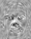
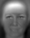
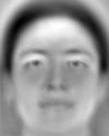
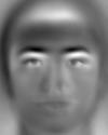
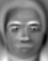
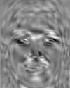
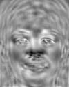
45 Face Representation using PCA and LDA Input face EigenFaces Fisherfaces PCA LDA Reconstructed face Minimize reconstruction error Maximize between-class to within-class scatter

46 Discriminant Analysis PCA finds components that explain data variance; the components may not be useful for discrimination between different classes Since no category label is used, components discarded by PCA might be exactly those that are needed for distinguishing between classes Whereas PCA seeks directions that are effective for representation, discriminant analysis seeks directions that are effective for discrimination Special case of multiple discriminant analysis is Fisher linear discriminant for C=

47 Fisher Linear Discriminant Given n d-dim samples x,..., x n ; n in the subset D labeled ω and n in the subset D labeled ω Find a projection that maintains separation present in the d-dim. space t y = wx Geometrically, if w =, each y i is the projection of the corresponding x i onto a line in the direction of w. The magnitude of w is of no significance, since it merely scales y Find w s.t. if d-dim samples labeled ω fall more or less into one cluster while those labeled ω fall in another, we want the projected points onto the line to be well separated as well

48 Fisher Linear Discriminant Figure 3.5 illustrates the effect of choosing two different values for w for a two-dimensional example. If the original distributions are multimodal and highly overlapping, even the best w is unlikely to provide adequate separation

49 Fisher Linear Discriminant Fisher linear discriminant is the linear function that maximizes ratio of betweenclass scatter to within-class scatter -class classification problem has been converted from the given d-dimensional space to one-dimensional projected space Find a threshold, i.e., a point along the one-dimensional subspace separating the projected points from the two classes

50 Fisher Linear Discriminant In terms of S B and S W, the criterion function J( ) can be written as A vector w that maximizes J( ) must satisfy for some constant λ, which is a generalized eigenvalue problem If S W is nonsingular we can obtain a conventional eigenvalue problem by writing

51 Fisher Linear Discriminant In our particular case, it is unnecessary to solve for the eigenvalues and eigenvectors of due to the fact that S B w is always in the direction of m -m. Since the scale factor for w is immaterial, we can immediately write the solution for the w that optimizes J( ):

52 Fisher Linear Discriminant When the conditional densities p(x ω i ) are multivariate normal with equal covariance Σ, the threshold can be computed directly from the optimal decision boundary (Chapter ) where w 0 is a constant involving w and the prior. Thus, for the normal, equal-covariance case, the optimal decision rule is merely to decide ω if Fisher s linear discriminant exceed some threshold, and to decide ω otherwise.

53 Multiple Discriminant Analysis Generalize -class Fisher s linear discriminant to c-class problem Now, the projection is from a d-dimensional space to a (c - )-dimensional space, d c

54 Multiple Discriminant Analysis Because S B is the sum of c matrices of rank one or less, and because only c of these are independent, S B is of rank c or less. Thus, no more than c of the eigenvalues are nonzero, and so the new dimensionality is up to (c-).

55 Multiple Discriminant Analysis The projection from a d-dimensional space to a (c-)-dimensional space is accomplished by c- discriminant functions If the y i are viewed as components of a vector y and the weight vectors w i are viewed as the columns of a dx(c ) matrix W, then the projection can be written as a single matrix equation The columns of an optimal W are the generalized eigenvectors that correspond to the largest eigenvalues in

56 Multiple Discriminant Analysis Figure 3.6: Three 3-dimensional distributions are projected onto twodimensional subspaces, described by a normal vectors w and w. Informally, multiple discriminant methods seek the optimum such subspace, i.e., the one with the greatest separation of the projected distributions for a given total within-scatter matrix, here as associated with w.

57 T Y = LDA T w X Y = w X Find a transformation w, such that the w T X and w T X are maximally separated & each class is minimally dispersed (maximum separation)

58 PCA vs. LDA PCA LDA Sample mean n n i = µ = å xi µ i = å x N xîw i i Mean for each class Scatter matrix S n å = ( x -µ)( x -µ) i= i i T S w S b c åå = ( x -µ )( x -µ ) i= x ÎC c å i= j i j i j i = N ( µ -µ)( µ -µ) i i i T T Within-class scatter Betweenclass scatter Eigen decomposition Sw = lw S S w - W B = lw Eigen decomposition Y = T w X X is transformed to Y using w

59 Principal Component Analysis (PCA) Example X={(4,),(,4),(,3),(3,6),(4,4)} Statistics µ S = [ ], é ù = ê ú ë û Solve the Eigen value problem Sw = lw

60 Linear Discriminant Analysis (LDA) Example X = {(4,),(,4),(,3),(3,6),(4,4)} X = {(9,0),(6,8),(9,5),(8,7),(0,8)} Class statistics µ = [ ], µ = [ ], µ = [ ] é ù é.89.0 ù S = ê, =.0 3. ú S - ê ú ë û ë û Within and between class scatter S B é7 54ù é ù = ê, ú SW = ê ú ë û ë û Solve the Eigen value problem S S w - W B = lw

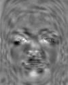
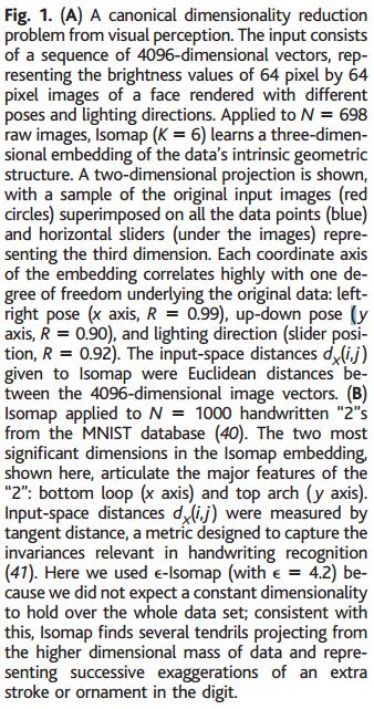
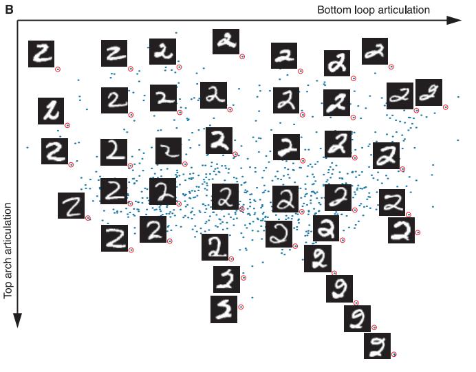
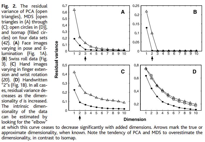
61 A Global Geometric Framework for Nonlinear Dimensionality Reduction Tenenbaum, de Silva and Langford, Science, V. 90, Dec 000 Although input dimensionality may be quite high (e.g for 64x64 pixel images in Fig A), the perceptually meaningful structure has many fewer independent degrees of freedom The images in A lie on an intrinsically 3-dim manifold, or constraint surface (two pose variables & an a lighting angle) Given unordered high-dim inputs, discover low-dim representations PCA finds a linear subspace; Fig. 3A illustrates the challenge of non-linearity; points far apart on the underlying manifold, as measured by their geodesic, or shortest path, distances, may appear close in high-dim input space, as measured by their straight line Euclidean distance.

62

63

64

65

66

67

68

69

70

71

72 Low Dimensional Representations And Multidimensional Scaling (MDS) (Sec 0.4) Given n points (objects) x,, x n. No class labels Suppose only the similarities between the n objects are provided Goal is to represent these n objects in some low dimensional space in such a way that the distances between points in that space corresponds to the dissimilarities in the original space If an accurate representation can be found in or 3 dimensions than we can visualize the structure of the data Find a configuration of points y,, y n for which the n(n-) distances d ij are as close as possible to the original similarities; this is called Multidimensional scaling Two cases Meaningful to talk about the distances between given n

73 Distances Between Given Points is Meaningful

74 Criterion Functions Sum of squared error functions Since they only involve distances between points, they are invariant to rigid body motions of the configuration Criterion functions have been normalized so their minimum values are invariant to dilations of the sample points

75 Finding the Optimum Configuration Use gradient-descent procedure to find an optimal configuration y,, y n

76 Example 0 iterations with J ef

77 Nonmetric Multidimensional Scaling Numerical values of dissimilarities are not as important as their rank order Monotonicity constraint: rank order of d ij = rank order of d ij The degree to which d ij satisfy the monotonicy constraint is measured by Normalize J to prevent it from being collapsed ˆmon

78 Overfitting

79 Problem of Insufficient Data How to train a classifier (e.g., estimate the covariance matrix) when the training set size is small (compared to the number of features) Reduce the dimensionality Select a subset of features Combine available features to get a smaller number of more salient features. Bayesian techniques Assume a reasonable prior on the parameters to compensate for small amount of training data Model Simplification Assume statistical independence Heuristics Threshold the estimated covariance matrix such that only correlations above a threshold are retained.

80 Practical Observations Most heuristics and model simplifications are almost surely incorrect In practice, however, the performance of the classifiers base don model simplification is better than with full parameter estimation Paradox: How can a suboptimal/simplified model perform better than the MLE of full parameter set, on test dataset? The answer involves the problem of insufficient data

81 Insufficient Data in Curve Fitting

82 Curve Fitting Example (contd) The example shows that a 0 th -degree polynomial fits the training data with zero error However, the test or the generalization error is much higher for this fitted curve When the data size is small, one cannot be sure about how complex the model should be A small change in the data will change the parameters of the 0 th -degree polynomial significantly, which is not a desirable quality; stability

83 Handling insufficient data Heuristics and model simplifications Shrinkage is an intermediate approach, which combines common covariance with individual covariance matrices Individual covariance matrices shrink towards a common covariance matrix. Also called regularized discriminant analysis Shrinkage Estimator for a covariance matrix, given shrinkage factor 0 < a <, S i ( a) = ( -a) nis ( -a) n i i + ans + an Further, the common covariance can be shrunk towards the Identity matrix, S ( b ) = ( - b ) S + bi

84 Principle of Parsimony By allowing the covariance matrices of Gaussian conditional densities to be arbitrary, the no. of parameters in the resulting quadratic discriminant analysis to be estimated for large d or C can be rather large In such situations, LDF is often preferred with the principle of parsimony as the main underlying thought Dempster (97) suggested that parameters should be introduced sparingly and only when data indicate they are required. A.P. Dempster (97), Covariance selection, Biometrics 8, 57-75

85 Problems of Dimensionality

86 Introduction Real world applications usually come with a large number of features Text in documents is represented using frequencies of tens of thousands of words Images are often represented by extracting local features from a large number of regions within an image Naive intuition: more the number of features, the better the classification performance? Not always! There are two issues that must be confronted with high dimensional feature spaces How does the classification accuracy depend on the dimensionality and the number of training samples? What is the computational complexity of the classifier?

87 Statistically Independent Features If features are statistically independent, it is possible to get excellent performance as dimensionality increases For a two class problem with multivariate normal classes P ( x w j ) ~ N( µ j, S), and equal prior probabilities, the probability of error is P( e) = p - u ò r where the Mahalanobis distance is defined as r e du T - = ( µ -µ ) S ( µ -µ )

88 Statistically Independent Features When features are independent, the covariance matrix is diagonal, and we have r = d å i= æ µ i - µ ç è s i i ö ø Since r increases monotonically with an increase in the number of features, P(e) decreases As long as the means of features in the differ, the error decreases

89 Increasing Dimensionality If a given set of features does not result in good classification performance, it is natural to add more features High dimensionality results in increased cost and complexity for both feature extraction and classification If the probabilistic structure of the problem is completely known, adding new features will not possibly increase the Bayes risk

90

91 Curse of Dimensionality In practice, increasing dimensionality beyond a certain point in the presence of finite number of training samples often leads to lower performance, rather than better performance The main reasons for this paradox are as follows: the Gaussian assumption, that is typically made, is almost surely incorrect Training sample size is always finite, so the estimation of the class conditional density is not very accurate Analysis of this curse of dimensionality problem is difficult

92 A Simple Example Trunk (PAMI, 979) provided a simple example illustrating this phenomenon. p( w ) = p( w ) = µ = µ,µ = -µ N p( X w ) ~ G( µ,i) p( x w ) = P e i= p p( X w ) ~ G( µ,i) N p( x w ) = P e i= N: Number of features p æ - ç xi - è æ - ç xi - è ö i ø ö i ø µ = i æ ç è i ö th ø = i component of the mean vector æ ö æ ö µ = ç,,,,... µ = ç-, -,-,-,... è 3 4 ø è 3 4 ø

93 Case : Mean Values Known Bayes decision rule: P t Decide w if x µ = x µ + xµ xn µ N x or P e e > - å = N i i i 0 > 0 z N = ò e dz æ ö g = µ - = å g / p µ 4 = ç i è i ø z ( N ) = e dz å ò N i= æ ö ç è i ø - p å æö ç è i ø is a divergent series ( N) 0 as \ N P e

94 Case : Mean Values Unknown m labeled training samples are available t Decide w if x µ ˆ = x ˆ ˆ... ˆ µ + xµ + + xn µ N P m i ˆ,{ i i i µ = å x x is replaced by - x if x Îw i= m Plug-in decision rule e > ( ) ( ) ( t ) ( ) ( t N, m = P w ˆ ˆ ). P x µ ³ 0 xîw + P w. P x µ ³ 0 xîw = P( x t µ ³ 0 xîw ) { due to symmetry t Let z = x µ N = å i = ˆ x i µ ˆ i POOLED ESTIMATE 0 It is difficult to computer the distribution of z

95 Case : Mean Values Unknown E lim N ( N, m) = P( z ³ 0 xîw ) P e P e N æ ö ( z) = å = ø i z - E VAR ç è i ( z) ( z) - z ( m, N ) = e dz ò lim P = 0 N N ~ G g / ( m, ) \ P e N N p lim = VAR ç æ + è ( 0, ), { Standard Normal ö m ø æö ç è i ø N ( z) = å = + ( z) ( z) æ ç z - E - E = P ³ è VAR VAR g N = - E VAR ( z) ( z) = i ( z) ö ( z) ø ç æ + è å ö m ø N m N i= å æ ç è c N i= ö ø ö + i ø æ ç è N m

96 Case : Mean Values Unknown

97 Component Analysis and Discriminants Combine features to increase discriminability & reduce dimensionality Project d-dim. data to m dimensions, m<<d Linear combinations are simple & tractable Two approaches for linear transformation PCA (Principal Component Analysis) Pattern Classification, Chapter 96 Projection that best represents the data 8

98 Diagonalization of Covariance Matrix Find a basis for which the components of a random vector X are uncorrelated It can be shown that the eignevectors of the covariance matrix for X form such a basis Covariance matrices (d x d) are positive semidefinite, so there exist d linearly independent eignevectors that form a basis for X If K is the covariance matrix, an eignevector e and an eignevalue a satisfy Ke = ae (K-aI)e = 0

99 y μ = [, ] é5 3ù Σ = ê 3 3 ú ë û x Eigenvectors: Eigenvalues: é ù ê ú ë û é ù ê ú ë û

100 Principal Component Analysis This can be easily verified by writing J 0 n å ( x ) = P( x -m)-( x -m) P 0 0 k k = n n n t åp( x0 m) P å( x0 m) ( xk m) åp( xk m) P k= k= k= = n n n t åp( x0 m) P ( x0 m) å( xk m) åp( xk m) P k= k= k= = n n åp( x0 m) P åp( xk m) P. k= k= = Independent of x 0 Since the second sum is independent of x 0, this expression is minimized by the choice x 0 =m.

101 Principal Component Analysis The scatter matrix is merely (n-) times the sample covariance matrix. It arises here when we substitute a k found in Eq. (83) into Eq. (8) to obtain n n n k k P k P k= k= k= å å å J () e = a - a + x -m n n t [ e ( xk -m)] åpxk -mp k= k= å =- + n n t t ( k )( k ) åp k k= k= å =- e x -m x -m e+ x -m n å t =- ese+ Px -mp. k = k P

102 Principal Component Analysis The vector e that minimizes J also maximizes e t Se. We use the method of Lagrange multipliers (Section A.3 of the Appendix) to maximize e t Se subject to the constraint that e =. Letting λ be the undetermined multiplier, we differentiate u with respect to e to obtain t t = ese-l( ee-) u = Se - le. e Setting this gradient vector equal to zero, e is the eigenvector of the scatter matrix: Se = le.

103 Principal Component Analysis Since e t Se = λ e t e = λ, it follows that to maximize e t Se, we want to select the eigenvector corresponding to the largest eigenvalue of the scatter matrix. In other words, to find the best one-dimensional projection of the d-dimensional data (in the least-sumof-squared-error sense), project the data onto a line through the sample mean in the direction of the eigenvector of the scatter matrix with the largest eigenvalue.

104 is minimized when the vectors e, e d are the d eigenvectors of S with the largest eigenvalues. Principal Component Analysis This result can be readily extended from a onedimensional projection to a d -dimensional projection (d <d). In place of Eq. (8), we write where d d. d ' = +å ai i i= x m e, It is not difficult to show that the criterion function J d' n d' å å ki i k k= i= = ( m+ a e )-x

105 Fisher Linear Discriminant How to find the best direction w that will enable accurate classification? A measure of the separation between the projected points is the difference of the sample means. If m i is the d-dimensional sample mean mi = å x, ni x Î then the sample mean for the projected points is ± mi = n i yîy i D i t t = å wx= wmi n i å xîd i y

106 Fisher Linear Discriminant The distance between the projected means is and we can make this difference as large as we wish merely by scaling w. To obtain good separation of the projected data we really want the difference between the means to be large relative to some measure of the standard deviations for each class. Define the scatter for projected samples labeled ω i by

107 How to solve for the optimal w? Fisher Linear Discriminant Thus, is an estimate of the variance of the pooled data, and is called the total within-class scatter of the projected samples. The Fisher linear discriminant employs that linear function w t x for which the criterion function is maximum (and independent of w ). The vector w maximizing J( ) leads to the best separation between the two projected sets.

108 y μ= [, ] é Σ= 5 0 ù ê 0 3 ú ë û x Eigenvectors: Eigenvalues: é ù ê ú ë û é ù ê ú ë û