convergence theorem in abstract set up. Our proof produces a positive integrable function required unlike other known

Transcription

1 218 Chapter 5 Convergence and Integration In this chapter we obtain convergence theorems. Convergence theorems will apply to various types of integrals and we are not required to prove them separately. We prove Monotone convergence theorem in abstract set up. Our proof produces a positive integrable function required unlike other known proofs valid for integral on real line using the existing positive integrable function on real line. We deduce a dominated convergence theorem for functions. The notion of equiintegrability and the relevant theorems will work in any integration apparatus. This is the virtue of our abstraction. We prove equintegrabilty theorem in a general setting We prove a more general form of dominated convergence theorem applicable for conditionally integrable mappings which may assume values in a Banach space or a metric semigroup. Our results are applicable to mappings taking fuzzy real values and to Aumann integral. Our results are applicable for both Henstock-Kurzweil integral as well as Mcshane integral. We have generalized results for the space of Henstock-Kurzweil integrable mappings to abstract set up. Throughout this chapter we assume that an integration apparatus (X, B, O, G) is set up, and premeasure is positive and additive.. Monotone convergence Theorem in Abstract Set up.

2 219 Definition [1] σ finite Cell:In an integration apparatus (X, B, O, G) set up. We say a cell B is σ finite, if there exists a strictly positive integrable function σ on B*\O with the integral I (B, σ) > 0. Examples [2] : 1) Any bounded cell is always σ finite, as the characteristic function 1 B is the strictly positive integrable unction. 2) R* is σ finite as the function is a strictly positive function defined on R. We have tan -1 ( ) = π/2 and tan -1 (- ) = - π/2. 3) R* R* is σ finite, as there exists a strictly positive integrable function on R R. Remark: If X is σ finite then any cell in B is σ finite. Lemma [ 3] : If σ is a strictly positive integrable function on X, then there exists a positive constant K > 0, and a gauge λ such that, 0 < S(P, σ) K, for any λ fine tagged partition P. Proof: Since the function is strictly positive, any Riemann sum is strictly positive. Select a gauge λ such that, S(P, σ) I < I/2. Hence I/2 < S(P, σ) < 3I/2. So we are done if K = 3I + 1. Remark: The result holds for any λ fine partial tagged partition. In any integration theory Monotone convergence theorem yields other convergence theorems like dominated Convergence theorem. In what follows we prove the results for mappings defined and integrable over X and these will hold for any cell B. It

3 220 should be noted that case (ii) of the step two in the proof of monotone convergence theorem, is not needed in case X is σ finite (that is in case of Euclidean spaces) as the required strictly positive function σ exists by default. Our proof is adapted from the papers [39], [40] and [ 11] but we produce positive integrable function and proof works for unbounded cells. It seems that another approach, possibly simpler may be available by using derivatives of set functions introduced by us in chapter 3, and a similar approach is used in the paper [ 12] but the argument there is applicable only for functions integrable on the real line. Theorem [ 4 ] Monotone convergence Theorem : Let f n be a sequence of monotone integrable functions defined on X, and f = lim almost everywhere. Then, f is integrable if and only if the sequence I(f n ) is bounded and in this case I ( f ) = lim. If f 1 is absolutely integrable then f is absolutely integrable. Proof: Without any loss of generality we assume that the sequence {f n } is increasing and converges everywhere. Only if Part : If f is integrable, then the sequence of integrals I(f n ) is a monotone increasing sequence bounded above by I(f). Thus we are done. If Part :

4 221 Step 1: Since the changes in the values of a function over a set of measure zero does not change the value of integral nor the integrability status, we assume that the functions f and f n are defined and finite everywhere on X.We also assume that f(x) and f n (x) = 0 for each pint in O, if X has infinite measure. By considering f n or f n f 1, we assume that the sequence f n is increasing, f n 0, for all n ℵ and I(f n ) < M for some positive constant M > 0. Since the sequence I(f n ) = I n (say) is monotone increasing ( that is non decreasing) and bounded above lim exits and we denote it by I. Step 2 : Case i) ( Applicable in particular when X = R* (real line ) or an Euclidean space) : If X is σ finite we note that there exists a strictly positive integrable function σ defined on X and a gauge λ such that, 0 S(P, σ) < K for some constant K > 0, for any λ fine tagged partition P of X. Case ii) X is not σ finite. Let E 0 = { x X f(x) = 0}. Let A = X \ E 0. Then there exists a gauge λ and a function σ, such that σ is strictly positive on A, 0 on E 0 and 0 S(P, σ) K, for any λ fine tagged partition P of X.

5 222 To show this we use the concepts defined in the article titled Henstock variation of functions, covered at a later stage in this chapter. Let for each n ℵ, E n = { x f n (x) 0, and f m (x) = 0, for m < n}.. Then A is disjoint union of E n. Since each f n is integrable and nonnegative each E n is vbg* by theorem [ 30], and hence A is vbg* being the countable union, by using theorem [34]. So by application of theorem [ 35], we get the desired function σ and the gauge λ. Step 3: Let I n = I ( X, f n )= I (f n ). Let I = sup { I(f n ) : n ℵ}, so that the increasing sequence I(f n ) denoted by I n converges to I. Given ε > 0, let r ℵ be such that, < ε and 0 < I - I r ε.(1) Since for each n ℵ, f n is Henstock-Kurzweil integrable, there exists a gauge δ n such that for any δ n fine tagged partition P, S(P, f n ) I n. (2) Since f n converges pointwise to f, for each x X, there exists an integer n(x) r, such that 0 f(x) f n(x) (x) ε. σ(x) (3), where σ is the function defined as in step 2. If f(x) = 0 at a point x in O, then let n(x) = r. Define a gauge δ as δ(x) = δ n(x) (x) λ(x), where λ is the gauge defined as in step 1.

6 223 Step 4: Let P = { (x k, J k ): k =1,2. m} be a δ fine tagged partition of X. Let S(P, f) = ). J k. We adopt the convention that blocks with infinite measure are included in the Riemann sum, the corresponding tag being point of O, belonging to the respective block of infinite measure, and we agree to say 0. = 0. We let (J k denote the indefinite integral ( a set function ) of over J k. SP, f) I ). J k - ). J k + - J + J - I. (4) The first term on the right hand side is equal to ε. S(P, σ) using (3) and as S(p, σ) < K by choice of σ, and as the gauge δ is finer than λ, we have first term < Kε. The second term on the right hand side is dominated by. (J k, ]. To estimate this term, let s = max{n(x k ) : k =1, 2 m }. Then s r, as n(x k ) r for all x k. We note that this finite sum can be written as iterated sum : first over all values of k such that, n(x k ) = p for some integer p r, and then sum over p = r,. s. Consider all those tags x k with n(x k ) = p, for fixed p. Each corresponding block J k is contained in δ(x k ) = = δ p (x k ). So the collection {(x k, J k ) : n(x k ) = p } forms a

7 224 δ p fine tagged partial partition. So by using Henstock s estimate [lemma 3.9 ], and inequality ( 2) we get,. (J k, ]. (5). If we sum the inequality in (5) over p = r,, s. we find that the second term in the right hand side of the inequality (4) is dominated by, = ε. We estimate the third term on the right hand side of the inequality (4). Since the sequence {f n } is increasing and r n(x k ) s, f r f s, I(J k, f r ) I (J k, ) I(J k, f s ). Summing these inequalities, for k =1, 2 m, we have, I r = I(f r ) I (J k, ) I(J k, f s ) = I s I. Using inequality (1), it follows that I ε I r I (J k, ) I. So the third term is also dominated by ε. Combining these estimates S(P, f ) I < ε.( K + 2), where K > 0 is a constant. So f is integrable with I (f ) = I. f f 1 0, and hence absolutely integrable.hence f = (f f 1 ) + f 1 is absolutely integrable, if f 1 is absolutely integrable. Another Proof We now offer another proof which is our original. First two steps are same as in the previous proof.

8 225 Step 3 : Let F n denote the indefinite integral of f n for each n ℵ. So F n ( D ) 0, for each cell F and { F n ( D ) } is a monotone increasing sequence of real numbers for each cell D. Define the set mapping, F, as F(D) = lim, for each cell D. Clearly F(D) 0, for each cell D and F(D) is finite. Step 4 :We now show that F is finitely additive for partitions. If { D k : k =1, 2 m} is a partition of cell D, then given ε > 0, there exists n k ℵ such that,f ( D k ) F n ( D k ) ε / m for n n k and there exists n 0 ℵ such that, F(D) F n (D) ε, for n n 0. Let p = max { n k : k = 0, 1, 2.. m}. F(D) - ) = F(D) - F p (D ) + F p (D) - So F(D) - ) = F(D) - F p (D) + - ε + / = 2 ε. Since F(D) and F(D k ) are fixed numbers and ε is arbitrary, we have shown that F is additive. Since f is nonnegative, F is nonnegative and G n = F F n is a nonnegative increasing set function for each n ℵ, that is G n ( D ) G n ( E ), if the cell E is contained in a Cell D. Thus if G n ( X ) ε, then for any set A which is a union of separated cells. G n (A) ε. Step 5 : Let ε > 0 be fixed. When x is a point at infinity, select a positive integer M, so that F(X) F M ( X ) ε, and set n(x) = M.

9 226 Using Henstock s Lemma select gauge δ M finer than λ so that, for any δ M fine tagged partial partition Q formed by all unbounded cells,,, =,, 2ε. ( 1 ) For any set A, which is a union of mutually separated cells, F(A) F M (A) ε ( 2 ) For each x X, which is not a point at infinity select positive integer n ( x ) M, with the property that f(x) f n (x) (x) ε. σ(x) and F(X) F n ( x ) (X) ε. σ(x) for n n ( x ). Using Henstock s Lemma,select gauge δ n(x) finer than λ, as well as δ M,, so that f n ( x ) (x). D - F n ( x ) (D) ε. σ(x), for each δ n(x) fine block D. Define a gauge δ on X as δ (x) = δ n ( x ) ( x ), for each x X. Step 5:Consider a δ fine tagged partition T ={( x j, J j ) : j = 1,2.. s} of X. Consider a typical bock say (x, J) in T, for some j, where x is not a point at infinity. J δ(x) = δ n ( x ). By division axiom we have a partition of X given by {K k : k = 0, 1,2 q }, with J = K 0 as a block. Using the gauge δ n(x), We can obtain a δ n(x) fine tagged partition of each block K k, k =1, 2.. q. Thus { (x, J) } is a δ n(x) fine tagged partial partition of X, and so we have, f n(x) (x). J - F n(x) (J) ε. σ(x).

10 227 This is valid for any block Jj in T. So for each block ( x j, J j ) in the tagged partition T, when x j is not a point at infinity, we have (x j). J j - (J j ) ε. σ(x). (3) Step 6 : Similarly Q = { ( x, J ) : x is a point at infinity and J is unbounded block in T. } forms a δ M fine partial tagged partition Q of X. We note that only bounded blocks contribute to Riemann sum. Let A be the set obtained by forming union of mutually separated unbounded cells in T occurring in the partial tagged partition Q. We see that that Riemann sum, S ( T, f ) =., 1 r s. We estimate, F ( X ) S (T, f) F ( X ) F M ( X ) + F M (X) S (T, f ) F (A) - F M (A ) +,, ε + ε + 2 ε + ε. S (T, σ ) + ε. S ( T, σ ) 4 ε + 2 K.ε. Since ε is arbitrary, and K is constant, f is integrable over X with integral as F(X). Another treatment of monotone convergence theorem

11 228 We offer an entirely different approach to the proof of monotone convergence theorem. the prrof is our original. A similar proof but valid only for closed bounded cell on real line is offered in [ ] Definitions [4 A] i) By a point cell mapping H we mean a mapping of the type, H(x, D) where x is a point and D is a cell. ii) Variation of a mapping H with respect to a gauge δ over a cell B : H can be a point mapping or a point cell mapping or a cell mapping. This is defined as, V δ (H) = sup { ( S(P, H ) : P is a δ fine tagged partition of B, S(P, H ) denotes the Riemann sum iii)variation of a mapping H over a cell B : H can be a point mapping or a point cell mapping or a cell mapping. This is defined as V(H, B) = inf { V δ (H) : δ is a gauge } iv) A cell mapping F(D) is said to be additive if, whenever P = { D 1, D 2, D n } is a partition of a cell D of finite measure, F (D) =. v) A cell function G(D) is said to be superadditive if whenever P = { D 1, D 2, D n } is a partition of a cell D of finite measure, G (D). Remark : For any point cell mapping H, V δ (H) is a superadditive cell function.

12 229 Definition [ 4B] : For a mapping f defined over X, with an associated additive cell mapping F and a cell D, we define the associated point cell mapping H f (x, D) as follows, H f (x, D) = F(D) D. f (x), if D is a bounded cell, else H f ( x, D ) = F( D), when D is an unbounded cell. Note : We drop the suffix f whenever the context is clear and simply write as H(X, D ) or simply as H. Theorem [4C] Reinterpretation of Henstock s lemma : Let f be a function defined over X ( recall f is 0 at each point at infinity). If f is integrable on X, then V(B, H) = 0 for any cell B. Proof : If f is integrable on X, given a cell B, select a gauge λ, using conformal partition lemma. So any λ fine tagged partition P of B contains a λ fine tagged partition P B of B. Since F is additive we have S(P B, H ) S ( P, H ). Thus by Henstock s estimate, given ε > 0 we have a gauge δ such that S(P B, H ) = V δ (B, H) < ε. Thus V(B, H) = 0. First we prove some preliminary results needed. Our treatment is inspired by [5] but substantially modified to suit abstract set up and bounded cells and uses gauges. Theorem [4D ] : Suppose f is a mapping defined over X. then f is integrable over X, with integral as F(X) and indefinite integral as F, if there exists a nonnegative superadditive cell function G, and

13 230 an additive cell mapping F such that, for a given ε > 0, there exists a gauge δ such that, for all x X, if a cell D δ(x), H(D) ε.g (D ) Proof : We claim f is integrable with indefinite integral F., we note that when D is an unbounded cell x k is a point at infinity and f ( x k ) = 0 S(P, f) F(X) =. - =, ε. ε G(X). Thus f is integrable and integral is F(B). Theorem [4E] Let f be an integrable function over X with F as an indefinite integral. Then there exists an additive cell function F and a superadditive nonnegative cell function G such that given ε > 0 there exists a gauge δ with the property that, for all x X, if D δ(x), H(D) < ε. G(D), with H(D) = F(D) D. f(x), where f(x) = 0 at a point at infinity in X. Proof : By Theorem [ 4C], V(B, H ) = 0, for any cell B. So given a natural number k ℵ, there exists a gauge δ k, such that, 2 - k, for any cell B. Define cell function G as G(B) =. B, H) for any cell B. Then G is nonnegative finite valued superadditive cell function.

14 231 Given ε > 0 we find k ℵ such that 1/ k < ε. Consider the gauge δ = δ k. For δ k fine tagged partition P, we have H(D), (1/ k).g(d) < ε.g (D). We now present the main result. Monotone convergence Theorem : If f n is a monotone increasing sequence of integrable functions converging pointwise to a function f, then f is integrable and I(f) = lim, provided the limit exists and is finite. Proof : Without loss of generality we can assume that each f n is nonnegative. Step 1 : Let F n denote the indefinite integral of f n for each n ℵ. So F n ( D ) 0, for each cell F and { F n ( D ) } is a monotone increasing sequence of real numbers for each cell D. Define the set mapping, F, as F(D) = lim, for each cell D. Clearly F(D) 0, for each cell D and F(D) is finite. Step 2 : We now show that F is finitely additive for partitions. If { D k : k =1, 2 m} is a partition of cell D, then given ε > 0, there exists n k ℵ such that,f ( D k ) F n ( D k ) ε / m for n n k and there exists n 0 ℵ such that, F(D) F n (D) ε, for n n 0. Let p = max { n k : k = 0, 1, 2.. m}.

15 232 F (D) - ) = F( D ) F p ( D ) + F p ( D ) -. Thus, F (D) - ) = F( D) F p (D) + - ε + / = 2 ε. Since F(D) and F(D k ) are fixed numbers and ε is arbitrary, we have shown that F is additive. Since f is nonnegative, F is nonnegative. Step 3 : Since f n is integrable, there exists an nonnegative superadditive cell function G n by theorem [ 5E], with the property that given ε > 0 there exists a gauge δ n such that for any tagged block (x, D) in a δ n fine tagged partition we have H n (D) ε. G n (D)., where H n (D) = F n (D) f n (x). D, and f n (x) = 0 for any point at infinity with G n is constructed as in theorem [5 E]. Replacing {f k } by a subsequence, if necessary we may assume that F k (X) > F(X) 2 k. Since (F - F k ) (D) (F F k )(E), if D E, we have F(D) F k (D) < 2 - k for any cell D. (1) We note that 0 G n 1 for all n ℵ. We construct cell function G as G(D) = 2. (D))+ S(D), Where S(D) = D }, if D is a bounded cell of finite premeasure, else S(D) = 0.

16 233 We note G is nonnegative and superadditive and by (1), G is finite. Given ε > 0, we find k ℵ such that 1/ k < ε and f(x) f k (x) < ε. Select the gauge δ = δ k. Consider a δ fine tagged partition P For a tagged block (x, D), H(D) = F(D) f (x). D, f(x) = f k (x) = 0 at a point at infinity. H(D) F k (D) f k (x). D + F(D ) F k (D) + R(D), Where R(D) = f(x) f k (x). D, when x is not a point at infinity, and R(D) = 0, when x is point at infinity that D is unbounded cell. F k (D) f k (x). D + (1/ k + ε ) G(D) ε. G k (D) + 2ε. G(D) 3ε. G(D). So f is integrable with indefinite integral F by theorem [4D]. The conclusion of monotone convergence theorem motivates us to make a definition. Definitions [ 5] : We say a function f is *integrable over a cell B with integral as, if given a real number K > 0, there exists a gauge δ such that for all δ fine tagged partitions P, S (P, f) >K. or if there exists an increasing sequence of functions f n converging to f almost everywhere such that lim =. We say a function f is *integrable over a cell B with integral as -, if given a real number K > 0, there exists a gauge δ such that for all δ fine tagged partitions P, S (P, f) < - K. or if

17 234 there exists a decreasing sequence of functions f n converging to f almost everywhere such that lim = -. We now deduce results in integration theory which follow from Monotone convergence theorem. Theorem [6]: Let f be a nonnegative function. Then I (B, f ) = 0 implies that f is zero almost everywhere on B* Proof : let A = { x B* : f(x) > 0 }. Suppose A is not of measure zero. Hence I (B, 1 A ) > 0. For each n ℵ, let A n ={x B* f(x) 1/n}. Then f. 1. So I (B,.1 I (B, f), but I(B, f) = 0 and as measure is complete, we have m(a n ) = I (B, 1 ) = 0, for each n ℵ. Since the set A = {x B*: f (x) 0 } is countable union of the sets A n, each having measure zero, it has measure zero by application of monotone convergence theorem after expressing it as increasing union of sets. Corollary [7]: Let f be a mapping, such that f is integrable and I ( f ) = 0, then f is zero almost everywhere. Proof : Follows immediately from the immediately preceding result as f is zero almost everywhere.

18 235 Theorem [ 8] : Daniell Property If f n is a decreasing sequence of nonnegative functions such that, I(f n ) 0, as n, then f n 0 as n, almost everywhere. Proof : Let f = lim = f. So f 0. By monotone convergence theorem I(f) = 0. Since f is nonnegative function f is zero almost everywhere by theorem 6. Remark: The next theorem shows that the assumption that the limit function exists almost everywhere in the hypothesis of monotone convergence theorem is superfluous but we need the monotone convergence theorem to deduce it. Theorem [ 9] Beppo Levi Theorem for sequences :- Suppose {f n : n ℵ} is a monotone sequence of integrable functions defined almost everywhere in X. Let the sequence {I(f n )} of integrals be bounded almost everywhere. Then, lim = f(x) is finite almost everywhere and f is integrable with I(f) = lim. Proof :- Without loss of generality we can assume f n nonnegative for each n ℵ and the sequence {f n } is increasing and convergent everywhere. Let I (f n ) K. Let Z = {x X: lim = }. For each r ℵ, define a sequence {g n } of functions as,

19 236 g n = min {, 1 }. By Monotone convergence theorem h r = lim is integrable and I ( h r ) K / r. If x Z, then h r (x) = 1, for all r ℵ. If x is not in Z, then f(x) < r for some r and hence lim = 0. So h 1 Z. Another application of monotone convergence theorem gives us, I (lim ) = I ( 1 Z ) = lim lim = 0. So Z is of measure zero, and f is finite almost everywhere. The second conclusion follows from Monotone convergence theorem. Theorem [ 10 ] Beppo Levi Theorem for series of functions : 1) If s n is a series of nonnegative integrable functions and the series I (s n ) is convergent, then s n converges almost everywhere and = I ( ). 2) If u n is a series of absolutely integrable functions and the series I ( u n ) is convergent, then u n converges almost everywhere and = I (. Proof : To prove (1), we apply the immediately preceding theorem to the sequence of partial sums given by f n =. We can deduce (2) from (1) by setting s n = u n + and t n = u n -. and applying the conclusion of (1) to s n and t n and noting that u n = s n + t n. Example [ 11] :- dx = =.

20 237 = 1 =. 1 Theorem [12] : Let f n be a sequence of integrable functions such that, h f n g, for all n, where g, and h are integrable functions, then, i) v = inf {f n ; n ℵ}, defined by v(x) = inf {f n (x) : n ℵ}, for each x X, and similarly the function u = sup { f n : n ℵ}are integrable, ii) I(v) inf {I(f n ): n ℵ} Sup{ I(f n ): n ℵ} I (u). Proof : The functions u n = sup {f 1, f 2,... f n }are absolutely integrable for each n, and they form an increasing sequence bounded above by g. So the sequence converges almost everywhere and by Monotone convergence theorem we get the result for u. Similarly result holds for v Lemma [13] Fatou s Lemma: Let {f n } be a sequence of integrable functions bounded below by an integrable function h, such that, lim inf I(f n ) <, then the function f defined as, f = lim inf f n is integrable and, - < I (lim inf f n ) lim inf (I(f n )) <. Proof : Let for each n ℵ, g n = inf {f m : m n }. The immediately preceding lemma implies that g n is integrable, for each n ℵ. Since h(x) g n (x) f n (x), for each x X, and n N, I(h) I(g n ) I(f n ). Hence I(h) lim inf I(g n ) lim inf I(f n ).

21 238 The sequence {g n } is an increasing sequence, converging to the function f = lim inf f n. So the increasing sequence of integrals I(g n ) is convergent and therefore bounded. So by Monotone convergence theorem f is integrable. I ( f ) = lim lim inf I(g n ) lim inf I(f n ). We now prove dominated convergence theorem for functions using Fatou s lemma. Another proof of the theorem for mappings assuming values in a Banach space or a metric semigroup is offered using the notion of equiintegrability separately. That proof is our original. Theorem [14] Dominated convergence Theorem for functions : Let {f n : n ℵ} be a sequence of Henstock-Kurzweil integrable functions converging to f almost everywhere on B*. Suppose there exists Henstock-Kurzweil integrable functions g and f such that, g(x) f n (x) h(x), for almost all x then f is Henstock-Kurzweil integrable over B, and lim, ) = I(B, f). Proof : Since f(x) = lim, f(x) = lim inf f n (x). Also I(g) I(f n ) I(h), for n ℵ, whence both lim inf{i(f n )} and lim sup {I(f n )} exist finitely. By Fatou s lemma f is Henstock- Kurzweil integrable, and I(f) lim inf {I(f n }.

22 239 We also apply Fatou s lemma to the sequence f n and note that lim inf I(-f n )} = -lim sup{i(f n )},we have I(f) - lim sup { I(f n )}. So I(f) lim sup {I(f n ) }. So we are done. The next result is deduced in Henstock-Kurzweil theory by us without using the notions of measurable set and integral over a measurable set. Theorem [ 15] Absolute continuity of the Indefinite integral: If f is an absolutely integrable mapping over X, then given ε > 0, there exists a real number δ > 0, such that, I (B, f ) < ε, whenever B is a bounded cell with B < δ. Proof: Without loss of generality we assume that f is a nonnegative function, as integral of f is considered. Consider the sequence f n = f n, for each n ℵ. It is a nondecreasing sequence converging to f. We hav f 1 f n f, for all n ℵ. Since f is integrable and f n is integrable we have I(f n ) I(f). So given ε > 0, there exists k ℵ, such that, I (f - f n ) < ε for n k. Let δ =. I(B, f) = I(B, f - f k) + I(B, f k ). Since f f k is a nonnegative function, I (B, f f k ) I ( f f k ) < ε/2, as the later integral is over X. Since f k k, I(B, f k ) k. B k.δ ε/2. Thus I ( B, f) < ε. Convergence theorems for mappings in a metric semigroup

23 240 Since the Henstock-Kurzweil integral is non absolute integral we would like a dominated convergence theorem valid for conditionally integrable mappings as well. This is achieved by the notion of equiintegrabilty. It is just as easy to study these notions for mappings assuming values in a metric semigroup with metric replacing the norm. We have offered proof of dominated convergence theorem for mappings in a metric semigroup. The papers [14], [15], [16] study integration for mappings into a metric semigroup but dominated convergence theorem is not presented there. We start with the familiar notion of uniform convergence. Definitions [ 16] Let B be a cell and f, as well as {f n : n ℵ} be a sequence of mappings defined over B*, assuming values in a metric semigroup E or in a Banach space E. i) We say a sequence of mappings {f n : n ℵ}, converges uniformly to a mapping f, in a metric space E, if the. Sequence d n = d (f n, f) = sup{ d(f n (x), (f(x) ) : x B*}, is convergent. Sup is if the set is not bounded above. ii) We say, a sequence of mappings {f n : n ℵ},converges uniformly almost everywhere to a mapping f, with an exceptional

24 241 set Z of measure zero, in metric space E, if the sequence, d n = d(f n, f) = sup{ d(f n (x), (f(x) ) : x B* \ Z}, is convergent. Sup is if the set is not bounded above. For a mapping g assuming values in a Banach space and defined over a set A X, we define, iv) g = sup { g(x) : x A}, if the sup exists and set it as otherwise. iv) A sequence of mappings {g n : n ℵ } defined over B*, assuming values in a Banach space is said to be uniformly convergent to a mapping g defined over B*, if given ε > 0, there exists M ℵ such that, g n - g < ε, for all positive integers, n M. We say g n g uniformly over B*. v) A sequence of mappings {g n : n ℵ } defined over B*, assuming values in a Banach space is said to be uniformly convergent to a mapping g defined over B*, almost everywhere if there exists an exceptional set Z of measure zero, such that g n g uniformly over A = B*\ Z. Remark : We are going to present results and mappings are assumed to be defined on B*. It is easily seen that the hypothesis holds for mappings assuming values in a Banach space

25 242 when mappings defined over B are extended to B*, by setting the value at any point in B*\ B as zero. Notation : In what follows we fix metric notation for this section as well as sections o regulated mappings, Riemann sum convergence theorem and equiintegrability until we prove the dominated convergence theorem We offer the proofs in settings of metic semigroup. if mappings atre assuming values in a Banach space one simply defines the metric d as d(f n (x), f m (x) ) = f n (x) f m (x) We note that d n = d(f n, f) = sup{ d(f n (x), (f(x) ) : x B* \ Z}. Theorem [ 17 ] Uniform Convergence Theorem : Let B be a bounded cell and {f n } be a sequence of integrable mappings converging almost uniformly to a mapping f, over B*., except for an exceptional set Z of measure zero.then f is integrable over B and lim, = I ( B, f). Proof :- Since Z is of measure zero, we change f n (z), and f(z) for all z Z and for all n ℵ, to a constant value say y z ( depends on z), without affecting the integrability status or value of integral for f, and f n, n ℵ so that convergence is uniform everywhere.

26 243 Let I n, = I (B, f n ), I = I(B, f ). Given ε > 0, there exists M ℵ, such that for all positive integers n, m M, d( f n, f m ) d( f n, f ) + d( f m, f ) < ε + ε = 2ε. Integrating over B gives us that I (B, d( f n f m ) ) 2 ε. B, for n, m M. Hence d (I n, I m ) 2 ε. B. So { I n : n ℵ } is Cauchy sequence, and hence it is convergent. Suppose it converges to I. Let ε > 0 be given and M be selected as above. For a tagged partition P of B, d(s[p, f], S[P, f n ]) (f(x j ), f n (x j )). J ε B. Fix positive integer r M, such that d( I r, I ) < ε. Select a gauge δ r such that, d (S[P, f r ], I r ) < ε, whenever P is δ fine. d (S[P, f ], I) ) d( S[P, f], S[P, f r ] ) + d (S[ P, f r ], I r ) + d (I r, I ) < ε. ( B + 2). Since B is constant and ε > 0 is arbitrary we are done. Regulated Mappings We introduce the concept of a regulated mapping, which is usually defined only over real line. However we innovate and allow a set of measure zero in the definition, as in abstract setting of integration apparatus we would like to define a continuous mapping and like to have the result that every continuous mapping is regulated. Unlike real line where only limit from right and limit

27 244 from left are the only choices, in abstract setting arbitrary choices are available. Since we want each step mapping to be integrable, in addition to the assumption that is a positive and additive semilattice we also assume that local Radon property holds. That is is an integration semilatttice for this section. See chapter 1, definition 43. It is clear that Set of discontinuities of a step mapping is a set of measure zero by the definition of step mapping, since intersection of any two separated cells is a degenerate cell. Definition [ 18] Regulated mapping : Let (X, B, O, G) be an integration apparatus. A mapping f defined over the closure B* of a cell B of X into a metric space E is called a regulated mapping over B*, if there exists a sequence {s n : n ℵ} of step mappings converging to f uniformly almost everywhere,on B*, except possibly for an exceptional set Z =., where Z n is the set of discontinuities of s n Remark : Since Z is of measure zero, by the preceding theorem a regulated mapping is absolutely integrable over a bounded cell. Definition [19] : Continuous mapping : Let B be a cell. A mapping f defined over B*, assuming values in a metric space

28 245 (E, d) is said to be almost everywhere continuous over B* except for an exceptional set Z of measure zero, if given ε > 0 there exists a gauge δ defined on X, such that d (f(x), f(y) ) < ε whenever y is inside (δ(x)), for x B*\ Z. Z is called as set of discontinuities of f. Theorem [ 20]: Let f be a regulated mapping defined over X. Then the set D of discontinuities of f is a set of measure zero. ii) Conversely any continuous mapping is a regulated mapping. Proof : Since f is regulated there exists a sequence {s n : n ℵ } of step mappings, converging to f almost uniformly that is except for the set Z =., where Z n is the set of discontinuities of s n We show f is continuous except for the exceptional set Z of measure zero. Given ε > 0, choose N ℵ such that d ( f(x), s N (x) ) ε, for all x X\ Z. Let x be a point not in Z. There exists a gauge δ N such that if y is inside (δ N (x)), then s N (x) = s N (y), s N being a step mapping and y is not a point of discontinuity of the step mapping s N. So y Z N and hence d (s N (y), f(y) ) ε. d(f(x),f(y)) d(f(x), s N (x) ) + d(s N (x), s N (y)) + d (s N (y), f(y)) 2ε. So f is continuous at x.

29 246 Step II converse part : Let f be defined and continuous over B*. We want to show that f is regulated over B*. We produce a sequence {s n :n ℵ} of step mappings having the desired property inductively. Let ε = 1. By continuity of f, there exists a gauge δ 1 such that, for x B*, d (f(x), f(y) ) < 1/n, whenever y is inside δ 1 (x). By Cousin s Axiom there exists a δ 1 fine tagged partition of B say P 1 = { ( x k, 1, K k, 1 ) : k =1, 2, d 1 }. For x K 1, 1 let s 1 (x) = f(x 1, 1 ). For x K 2, 1 \ K 1, 1, let s 1 (x) = f(x 2, 1 ). Continuing for x K m, 1 \ ( K 1,1,., K m-1,1 ), let s 1 (x) = f(x m, 1 ) for m =3, 4,, d 1. Let Z 1 be the set of discontinuities of s 1. Let ε = ½, By continuity of f, and by intersection property of gauges there exists a gauge δ 2 finer than δ 1 such that, for x B*, d (f(x), f(y) ) < 1/2, whenever y is inside (δ 2 (x)). By Cousin s axiom there exists a δ 2 fine tagged partition of each K k, j, j =1,2,., d 1. So we get a δ 2 fine tagged partition P 2 of B, which is a refinement of P 1 given by P 2 = { (x k, 2, K k,2 ) k =1,2,., d 2 d 1.}

30 247 We construct a step mapping s 2 based on this partition as we constructed s 1. Let Z 2 be the set of discontinuities of s 2. We continue this process for each n ℵ to obtain a sequence {s n n ℵ} of step mappings. Let Z =. Z is of measure zero. Let ε > 0 be given. Select the smallest positive integer N such that 1/N < ε. Let n N. For x Z, suppose x (K k, n ),for the least integer k {1,2,, d n }. d ( f(x), s n (x) ) d (f(x), f(x k, n ) ) < ε. So we are done. Corollary [ 20 A] : Let B be a bounded cell. A regulated mapping f defined over B* is integrable over B. If f is a mapping into a Banach space then f is absolutely integrable. Proof : By definition of a regulated mapping and uniform convergence theorem [Theorem 20] f is integrable. If f is a regulated mapping into a Banach space, then f is also a regulated mapping. Corollary [ 20 B] : Let B be a bounded cell. A mapping f which is continuous almost everywhere on B* is integrable over B and if f is a mapping into a Banach space then f is absolutely integrable. Proof : f is a regulated mapping and hence result follows.

31 248 Corollary [ 20 C] : Every monotone function defined over a closed bounded interval [a, b] R is absolutely integrable. Proof : A monotone function is a regulated function. The following notion is adapted from the paper [8]. The paper [34] is also consulted. The paper [ 34] compares the notion with the notion of equintegrabilty and uses the concept of convergence in directed sets (nets) to derive a general iterated limit theorem. These papers deal with integrals on bounded intervals on the real line. Riemann sum convergence notion Theorem [21] Convergence based on Riemann sums : Let B be a cell Let {f n } be a sequence of integrable mappings defined over B*, converging to a mapping f almost everywhere on B*. Then, f is integrable over B with I(B, f) = lim,, if and only if, for given ε > 0, there exists a positive integer n ε such that, for each n n ε, there exists a gauge δ n such that, for a δ n fine tagged partition P of B, d ( S[P, f n ], S[P, f ] ) < ε. Proof : let I n denote the integral I(B, f n ), for each n ℵ. We first show that I n is a Cauchy sequence. Let n ε be as specified in the theorem and a gauge δ n is obtained for each n n ε having the property that for any. δ n fine tagged partition P of B, d ( S[P, f n ], S[P, f] ) < ε.

32 249 Since f n and f m are integrable there exists gauges λ n and λ m respectively, so that for any λ n fine tagged partition P, d (S[P, f n ], I n ) < ε, and for any λ m fine tagged partition P, d ( S[P, f m ], I m ) < ε. Select a gauge λ ε = δ n δ m λ m λ n. For any λ ε tagged partition P of B, d(i n, I m ) d (S[P, f n ], I n ) + d (S[P, f n ], S[P, f] ) + d (S[P, f], I m ) + d (S[P, f m ], I m ) < 4ε. So I n is Cauchy sequence.and hence converges to say I. Now we show f is integrable and I= I(B, f). Let the notation be same. Let M be the positive integer such that, d(i n, I) < ε for all n M. We can select n ε large enough so that n ε M. Fix n n ε. Let a gauge δ ε be selected so that δ ε = δ n λ n. For any δ ε fine tagged partition P, we have, d (I, S[P, f]) d(s[p, f n ], S[P, f] ) + d ( S[P, f n ], I n ) + d (I n, I) < 3ε. So f is integrable with value of integral as I. Converse : Let f be integrable. Since I n I given ε > 0, there exists a positive integer n ε, such that, d(i n, I) < ε for all integers n n ε. Fix n n ε. Since f n is integrable there exists a gauge δ n such that, d(s[p, f n ], I n ) < ε, whenever P is a δ n fine tagged partition of B. Since f is integrable there exists a gauge δ ε such that,

33 250 d (S[P, f], I) < ε, whenever P is a δ ε fine tagged partition of B. Let δ = δ n δ ε. d(s[p, f], S[P, f n ]) d(s[p, f], I) + d (I, I n ) + d(i n, S[P, f n ]) < 3ε, whenever P is a fine tagged partition of B. The example is taken from [ 11] Example [22]: Let B = [0, 2] on real line. f n (x) = n, for x A n = (, + ], and 0 otherwise. Then f n the zero function, as n. f n is integrable with I n =. Define the gauge δ n by the gauge function, δ n (x) = ½. d ( x, {, + }, if x [ 0, 2] \ {, + }, And δ n (x) =, otherwise. Clearly the dominated convergence theorem does not apply. But S(P, f n ) 3/n and hence tends to 0 as n. So this is an illustration of the preceding theorem. Equiintegrability Definition [23] Family of Equintegrable mappings : Let B be a cell. A family H of mappings defined over B*, is said to be equiintegrable if for each ε > 0, there exists a gauge δ such that, d (S[P, f], I(B, f)) < ε, whenever P is any δ fine tagged partition, and f is any mapping in H.

34 251 The results from the papers [32], [ 33], [39], [41],[74] are adapted to abstract set up. We have modified the proof so that it suits the abstract set up and one does not have to assume the existence of a positive integrable function. We assume that is a positive and additive semilattice. Theorem [24] Equiintegrability Theorem: Let{ f n : n ℵ} be equiintegrable sequence of mappings defined over B*, converging to a mapping f pointwise on B*. Then, f is integrable over B and,i(b, f) = lim lim. Proof: Step 1: Let ε > 0 be given. Let δ be a gauge on B such that, for any, n ℵ, and for any δ fine tagged partition P, d (S[P, f n ], I (B, f n ) ) < ε / 3. Claim : We fix a δ fine agged partition P. There exists M ℵ such that, d (S [P, f j ], S[P, f k ]) < ε/3, whenever j, k M. Proof of the claim: If the cell B is unbounded then points at infinity in O do not contribute to Riemann sum, and Riemann sum includes only blocks of finite measure. Let{(x i, D i ), i =1, 2.. r } be the collection of bounded blocks in the fixed tagged partition P. Let V be the total measure of the collection of bounded blocks. Since f n f pointwise there exists M ℵ such that,

35 252 d(f j ( x i ), f k (x i ) )., for j. k M. So d(s[p, f j ], S[P, f k ] ), ). D i... V = ε /3, for j, k M. We now have, d (I(B, f j ), I(B, f k )) d(s[p, f j ], I(B, f j )) + d (S[P, f j ], S[P, f k ]) + d(s[p, f k ], I(B, f k )) < ε/3 + ε /3 + ε/3 = ε. Hence lim, exists and we denote it by I. Step 2 : Let T be any δ fine tagged partition. As in Step 1, we pick M ℵ,such that d (S[T, f M ], S[T, f]) < ε/3 and d (I, I(B, f M ) ) < ε/3. d(s[t, f], I) d(s[t, f M ], S[T, f]) + d(s[t, f M ], I(B, f M ))+ d(i, I(B,f M )) ε/3 + ε /3 + ε/3 = ε. Hence f is integrable and I (B, f) = lim, = I Remark [25] : Equintegrability is a concept which does not go well with the concept of almost everywhere convergence. Here is an example on real line. Let f n = 0 on B = [ 0, 1]. Then f n converges to the zero function and {f n : n ℵ is an equiintegrable sequence.but Consider g n, defined as g n (0) = n, and g n (x) = 0 at x 0. Then g n is almost everywhere equal to f n, for each f n ℵ, but {g n } is not an equiintegable sequence. To see this

36 253 suppose given ε > 0, there exists a gauge δ, such that, S(P, g n ) 0 < ε for all δ fine tagged partitions P. Define a gauge λ such that, λ(0) = δ(0), and for x (0, 1] λ(x) = min {δ(x), x 0 } Then any λ fine tagged partition P is a δ fine tagged partition and 0 must be a tag for a subinterval J which contains 0. We see that, as n,s(p, g n ). Definition [26] Equi gauge Cauchy sequence : A sequence {f n } of integrable mappings defined over B*, is said to be equigauge Cauchy, if for every ε > 0, there exists a gauge δ, and M ℵ, such that, for j, k M, d (S [P, f j ], S[P, f k ] ) < ε, for any δ fine tagged partition P. Theorem [27] Cauchy condition for equiintegrability: A sequence {f n } of integrable mappings is equi gauge cauchy over a cell B, if and only if it is equiintegrable on B and lim (, ) exists. Proof: Step 1: Suppose the sequence { f n } is equi gauge Cauchy. Let ε > 0 be given. Let δ be a gauge and M ℵ be such that, d (S[P, f j ], S[P, f k ]) < ε/3, for j, k M and δ fine tagged partition P. Consider a gauge μ such that, d (S[P, f j ], I(B, f j )) < ε/3 and d (S[P, f k ],I(B, f k ) < ε/3, for any μ fine tagged partition P. Let α

37 254 be a gauge defined by δ μ. Then for any α fine tagged partition T, d(i (B, f j ), I(B, f k )) d (S[T, f j ], I(B, f j )) + d (S[T, f j ], S[T, f k ]) + d(s[t, f k ], I(B,f k )) < ε/3 + ε/ 3 + ε/3 = ε. So I(B, f n ) is a Cauchy sequence and hence convergent. Step 2: Pick N ℵsuch that, d (I(B, f j ), I(B, f k )) < ε/3, for j, k N. Take a gauge λ such that, d(s(t, f N ), I(B, f N )) < ε/3, whenever T is an λ fine tagged partition of B. Set gauge ξ, as ξ = λ α, where α is a gauge as in step 1. For any ξ fine tagged partition T of B and for k N, We have d(s[t, f k ], I(B, f k )) d(s[t, f k ],S[T, f N ]) + d(s[t, f N ], I(B, f N )) + d(i(b, f N ), I(B, f k )) < ε/3+ ε/3 + ε/3 = ε. So equintegrability of the sequence is established. Converse: Let δ be a gauge such that d(s[p, f k ], I(B, f k ) ) < ε/3, for any δ fine tagged partition P of B and any k in ℵ. Select M in ℵ such that, d ( I (B, f j ), I (B, f k ) ) < ε/3, for j, k M. Hence, d(s[p, f j ], S[P, f k ] ) d( S[P, f j ], I(B, f j ) ) + d(i(b, f j ), I (B, f k )) + d (S[P, f k ], I(B, f k )) < ε/ 3 + ε/3 + ε/ 3 = ε. We give our new result.

38 255 Theorem [ 28] Dominated convergence theorem for Mappings into a metric semigroup : Let {f n } be a sequence of integrable mappings over X, converging point wise to a mapping f almost, everywhere. Let for all j, k ℵ, the functions d k, j = d(f k, f j ) = d (f j (x), f k (x)) be integrable with d k, j g, where g is an integrable function over X. Then, (i) The sequence {f n } is equiintegrable over X, (ii) f is integrable over X, (iii) lim ( lim. Proof: The proof is an adaptation of the technique used for the proof of the same theorem in [47] for lebesgue integrable mappings to suit the modified hypothesis. Without loss of generality we assume that convergence is at each point. Step 1 Set h m, n = j, k { d (f j,f k ), where n j k m}. That is h m,n (x) = sup{d(f j (x), f k (x) ) : n j k m }, for each x. Then each h m,n is integrable function. Fix n ℵ. For each n, the sequence h m. n, m = 1, 2. is an increasing sequence, converging to the function, say, H n = j, k { {d(f j, f k ) : where n j k}. H n g, by hypothesis. By Monotone convergence theorem each H n is integrable and one

39 256 has I(H n ) I(g). The sequence H n is monotone decreasing sequence decreasing to the zero function. By monotone convergence theorem the sequence of integrals is decreasing and I(H n ) 0. Step 2 Let ε>0 be given. Then there exists a natural number M ℵ such that, I(H n ) < ε/2, for all n M. We have a gauge δ such that for any δ fine tagged partition P, d (S[P, H M ], I(H M )) < ε/2. Let j, k M and P be a δ fine tagged partition. We have, by definition of H M, d(s[p, f j ], S[P, f k ]) S[P, d(f j, f k )]) S(P, H M ) I(H M ) + ε/2 < ε. So {f n : n ℵ} is equi gauge Cauchy. So Cauchy condition for equi integrability gives us (i) and this in turn gives us the other conclusions by the application of equi integrability theorem. We now focus our attention on mappings assuming values in a Banach space and revert to Banach space norm notation from the metric notation. Theorem [29] Dominated convergence theorem for Mappings in a Banach space : Let {f n } be a sequence of integrable mappings over X, converging point wise to a mapping f almost, everywhere. Let for all j, k ℵ, the functions f k - f j be integrable with f j f k g, where g is an integrable function over X. Then, (i) The sequence {f n } is equiintegrable over X,

40 257 (ii) f is integrable over X, (iii) lim ( lim. Proof: The proof follows from the immediately preceding theorem. Henstock Variation of mappings We define the concept of variation. Variation is an extended real valued nonnegative function. Even if a mapping is not integrable, variation of the mapping always exists. Thus variation is a generalization of the concept of measure and outer measure. We assume mapping f is defined on X and define variation of f on X. On real line we have mappings of bounded variation. Similarly we consider generalized bounded variation. These notions are taken from [ 59 ],[60] and [39]. Definitions [30] : For any nonempty subset E of X, and a mapping f defined over X, we define the mapping f E = f.1 E = f(x), if x is in E, and 0 when x is not in E. Consider f to be a mapping defined on X and δ be a gauge. Let F denote the indefinite integral of f when it exists. a) Variation of a mapping f on X, relative to a gauge δ: It is denoted by V(δ, f), and it is defined as, V(δ, f) = sup { S( P, f ) : S(P, f ) is the Riemann sum, for f for an arbitrary δ fine tagged partition P of X }.

41 258 b) Variation of a mapping f on a nonempty set E, relative to a gauge δ: This is denoted by V(δ, f, E) and defined as V(δ, f, E) = V(δ, f E ). c) Henstock Variation of a mapping f on X: This is denoted by V(f) and defined as, V(f) = inf { V(δ, f) : δ is a gauge on X}. d) Henstock Variation of a mapping f on E: This is denoted by V(E, f) and is equal to V(f E ). e)variation of a set E : This is denoted by m*(e) and is equal to V(X, 1 E ). f) A mapping f is said to be vbg on a set E, if V(E, f) is finite. g) A nonempty set E is said to be vbg, if its characteristic function 1 E is vbg on X, that is m*(e) is finite. h) A mapping f is said to be vbg* on a set E, if E can be expressed as countable union, E =, such that, f is vbg on each E n. i) A nonempty set E is said to be vbg*, if E can be expressed as a countable union of sets each of which is vbg. j) A nonempty set E is said to be almost vbg*, if E can be expressed as a countable union of sets,, E =, each E n, for n ℵ is vbg, and f is zero on E 0. Remark [31] : Following assertions follow immediately from definitions. If A B, then V(A, f) V(B, f) and m*(a) m*(b)

42 259 Let A B. If B is vbg ( respectively vbg*) then A is vbg ( respectively vbg*). Theorem [32] :For a mapping h, if h is integrable over a cell B, then h has finite Henstock variation on B*, V(B, h) = I (B, h ). Proof : Suppose h is integrable over B with integral as I. Given ε > 0, there exists a gauge δ such that, S ( P, h ) - I ) < ε, for all δ fine tagged partitions P of B. Select a gauge δ 1 finer than δ, so that S(T, h ) > V( δ 1, h, B) ε, for all δ 1 fine tagged partitions T. Then select a gauge δ 2 finer than δ 1 so that, for any gauge μ finer than δ 2, we have V(μ, h, B) < V(B, h) + ε, by using definition of variation, Then for any μ fine tagged partition T of B, we have, I - V(B, h) I S(T, h ) + S(T, h ) -V(μ, h, B) + V(μ,h, B) V(B, h ) ε + ε + ε = 3ε. So our assertion is proved. Corollary [ 33] : i) For any cell B of finite measure, m(b) = B = m*(b). ii) For any nonempty measurable subset E of finite measure, m(e) = m*(e). Proof :- We prove the second assertion. Since E is measurable if E has finite measure, 1 E is integrable on X and m(e) = I(X, 1 E ) = v(x, 1 E ) = m*(e). First assertion can be proved similarly

43 260 Theorem [34] : If f is a nonnegative integrable mapping defined on a nonempty set E, then E can be expressed as a disjoint union E=, and each E n, n ℵ is vbg, while f vanishes on E 0. The set A = is vbg* and E is almost vbg* Proof: let E n = { x E n-1 < n } for n ℵ, and E 0 ={ x E f(x) = 0}. Then m*(e n ) = V( 1 n.v(f, E n ) n.v(f, X). Since f is nonnegative integrable function for a fixed n, the term n. V(f, X) is finite. Hence m*(e n ) is finite for each n ℵ. So each E n, for n ℵ is vbg. Remark : It is remarked in [ 47] that measure theory has built in ơ finiteness. Likewise the Henstock-Kurzweil integration theory has built in ơ finiteness. Theorem [35] Existence of a nonnegative integrable function whose Riemann sums are bounded. Suppose X is almost vbg*, that is X is expressed as disjoint union, X =. Where m*(e n ) is finite for each n ℵ. Then there exists a nonnegative function σ defined on X, and a gauge λ on X such that, S(P, σ) < 1 for any fine tagged partition P of X, and σ is nonzero on each E n, n ℵ.

44 261 Proof : Let X =, where m*(e n ) is finite for each n ℵ. We define σ(x) as σ(x) =., for n ℵ and σ(x) = 0 for x E 0. For each n N, we can select a gauge δ n such that, V(δ n, 1 ) < m*(e n ) +. So V(δ n, σ.1 ) <, that is S(P, σ.1 ) <, for any δ n fine tagged partition P of X, as variation for a gauge is the sup of Riemann sums. Select a gauge δ such that, for x E n, δ(x) = δ n (x) and δ is arbitrary for x E 0. Let P be a δ fine tagged partition. Then since the Riemann sum contains only finitely may well defined terms there exists a largest integer k such that, S(P, σ) contains k terms. S(P, σ) = SP, σ. 1,(where S(P, σ) is grouped according to tags occurring from E n. ) < < 1. *Definition [36] Riemann sum and Integral of a point cell mapping: Let an integration apparatus (X, B, O, G) be set up. Let h be a point cell mapping that is a mapping h(x, K, y, N) where K is a cell, x is a tag of K, y is any other point associated with K and N is a positive integer associated with K. We define the Riemann sum corresponding to a tagged partition P of B given by, P = { (x k, K k ) : k= 1, 2.. n} as S(P, h) =,,,.

45 262 We say h is integrable over B with integral as H(B), if given ε > 0 there exists a gauge δ such that S(P, h) H (B) < ε, for any δ fine tagged partition P of B. *Remark [37 ] : 1) It is not necessary that all parameters in h are required to be present. For a point mapping f, only the parameter x is present, for a set mapping F only the parameter cell K is present, the parameters point y and integer N, associated with a cell K are usually absent. Reformulation of the definition of integral of a point mapping f defined over X [ 38 ] : We say f is integrable over X if given ε > 0, there exists an mapping F defined over cells and additive over cells, such that, for any δ fine tagged partition P of X, S(P, f) S(P, F) = S( P, f F) < ε. *Theorem [ 39]:- Suppose H is a finitely subadditive cell function. If for a cell B, for some gauge δ, the supremum of the set of Riemann sums, { S(P, H): P is a δ fine tagged partition of B } is finite and is equal to c, then H is integrable and I (B, H) = c. If there does not exist any gauge δ for which the supremum exists and is finite, then for each n ℵ, there exists a gauge δ n such that, S(P, H) n, for all δ n fine tagged partitions P.

46 263 Proof :- Suppose δ is the gauge as stated in the hypothesis. Then for a given ε > 0, there exists a δ fine tagged partition P of B such that c-ε < S(P, H) c, as c is the supremum over all δ fine tagged partitions. If we take a gauge µ which conforms to each block of δ, then for any µ fine tagged partition T, S(T, H) S(P, H) as union of blocks of T gives us blocks of P, and H is cell function and sub additive. But T is also δ fine thus c - ε S(P, H) S(T, H) c. Since This inequality holds for all µ fine tagged partitions, H is integrable and the integral is c. On the other hand Suppose for no gauge the supremum is finite. So for each n ℵ, there exists a gauge µ n with the property that there exists a µ n fine tagged partition T, such that S(T, H) n. Select a gauge δ n conforming to the blocks of µ. By finite subadditivity of F, for all δ n fine tagged partitions P, S(P, H) S(T, H) n. *Theorem [40]: If f is integrable function over a cell B, and if f has finite Henstock variation on B*, then f is absolutely integrable on B and on each cell E contained in B, with the property that, F(E) V (E, f ) = V(E, F). Proof : - for any tagged partition P, of any cell E contained in B, S(P, f ) S(P, F ) S (P, f F ) S(P, f F ) (1).

47 264 By Henstock s estimate, for a given ε > 0. There exists a gauge δ such that For any δ fine tagged partition partial P, S(P, f F ) < ε. Since f has finite variation, by (1), V(E, f) = V(E, F). For any cell E contained in B. Since F is indefinite integral, F is finitely additive and F is finitely subadditive. Variation of f and thus variation of F is finite. So by the preceding theorem F is integrable over E and it s integral over E is V(E, F) as F is nonnegative. Also as F is subadditive, F(E) I(E, F ) = V(E, f). By inequality (1) f is integrable over any cell E, contained in B. *Definition [41] : Two point cell mappings h 1 and h 2 are variationally equivalent if their difference h = h 1 h 2 has variation zero. Remark : If f is integrable, with indefinite integral F then f and F are variationally equivalent, as f F is integrable with integral zero, since given ε > 0, there exists a gauge δ, such that, S(P, f - F) < ε. *Theorem [42] Let B be a cell. If a mapping f (or a point cell mapping h) has variation 0 on B* then f ( respectively h ) is absolutely integrable over B, with the integral equal to 0, and the integral of f = 0.( respectively Integral of h =0.)

48 265 Proof :- Suppose V(B, f) = 0. Hence there exists a gauge δ such that, V(δ, f) < ε for a given ε > 0, Hence given ε > 0 for all δ fine tagged partition P, S(P, f ) S(P, f ) - 0 < ε. *Alexiewicz norm for Henstock-Kurzweil integrable mappings In this article we shall introduce Alexiewicz norm for Henstock-Kurzweil integrable mappings defined over B* given a a cell B. We assume that the semilattice is positive additive and satiffies local radon property, integration apparatus is Henstock-Kurzweil apparatus and integral is Henstock-Kurzweil integral. The norm was first introduced for Denjoy integrable functions in the paper [1]. We have obtained general results rather than restricting ourselves to the case of a bounded closed interval on the real line. Our results are based on and adapted from the papers [ 1], [82] and [45 ], [50]. In [50] a uniform version of Hemstock s lemma is presented for Euclidean spaces which is very useful in dealing with the space of Henstock-Kurzweil integrable functions. In this article Definition [43]: Let B be a cell in an Henstock-Kurzweil integration apparatus defined over a set X. We define KH(B, Y) to be the collection of Henstock-Kurzweil integrable mappings over

49 266 B, assuming values in a Banach space Y. Mappings are defined over B*. Theorem [44] : KH(B, Y) is a normed linear space under the Alexiewicz norm defined as f kh = sup{ I (D, f) : D is a cell contained in B.}. Proof : Proof is transparent from properties of the integral. By corollary to Henstock s lemma [ Chapter 3, corollary 11], if f kh = 0 then we have that I (B, f ) = 0 and hence f is equal to zero almost everywhere. Remark [45] : KH(B, Y) is not complete. It can be intuitively seen that the completion is in space of distributions. Let f n be a mapping on [0, ] defined as f n [x] = n, when x in [0, 1/n] and 0 otherwise. Clearly each f n is integrable with integral 1. As n, f n approaches the generalized function known as Dirac delta function. But this is not defined as a function in the usual sense, as the value of Dirac Delta function is at 0 and 0 elsewhere, whereas integral of the Dirac delta function over [0, ] = 1. We formalize this observation in a specific case. Theorem [ 46] : The space KH[ [0, 1], R* ] is not complete. Proof : Let F be a continuous nowhere differentiable function, defined over [0, 1] and F(0) = 0. For an example of such a function

50 267 see [30, page 256 ]. By Weirstrass approximation theorem (please refer [30]) the continuous function F can be uniformly approximated by a sequence, of polynomials {F n }. By Fundamental theorem of calculus F n (t) =, 0, 1. So F n is a Cauchy sequence under Alexiewicz norm. If there exists f in KH([0,1], R*) such that, F n converges to f under Alexiewicz norm then this implies, uniformly for on [0, 1]. This means that F(t) = differentiable almost everywhere.this is a contradiction.. So F is Now we show that step mappings are dense in KH(B, Y) under Alexiewicz norm. The proof rests upon division axiom and separation property. Theorem [ 47]: The Step mappings are dense in KH(B, Y). Proof : Let f be an integrable mapping and ε > 0 be given. Let D be a cell contained in B. By division axiom we can have a partition of B which contains D as a block, say {D = B 0, B 1,B 2,... B n }. So using conformal partition lemma [Chapter 2, Lemma 40 ] we have a gauge δ such that for any tagged δ fine partition P of B, there exists a δ fine tagged partition T which conforms to D and S(P, f) = S(T, f). Let Q be the tagged partial partition of T which

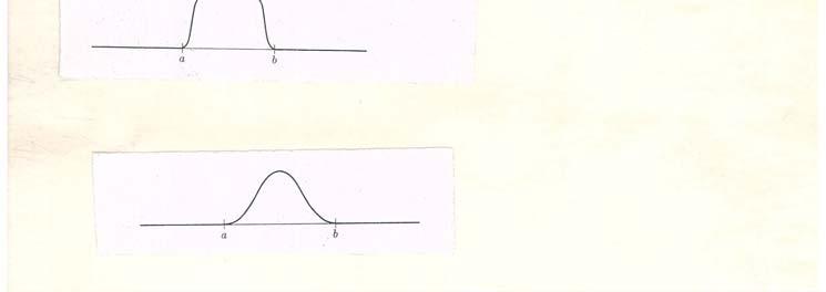
51 268 forms a tagged partition of D. Let λ be a gauge finer than δ so that for any λ fine tagged partition T= {(x j, J j ), 1 j n} of B, S(T, f) I(B, f) < ε. Let Q denote the associated λ fine tagged partition of D, formed as above. Let s be the step mapping formed by s =.. Then S(Q, f) I(D, s) ε by Henstock s lemma. [chapter 3, Lemma 9] So result follows from the definition of Alexiewicz norm. Theorem [ 48] C c functions are dense in KH(X, R*) where X is Euclidean space and Henstock-Kurzweil integral is considered. Proof : Let χ be the characteristic function of a rectangle. Then χ can be approximated from below and above by C functions, ψ and φ sp that 0 ψ χ φ < 1 so that I(B, φ - ψ) < ε for a given ε Proof uses Riemann integral. The proof is visualized in figure 1. For details of proof please refer ( see pp of [47 ] ).

52 269