Econometrics Lecture 1 Introduction and Review on Statistics

Transcription

1 Econometrics Lecture 1 Introduction and Review on Statistics Chau, Tak Wai Shanghai University of Finance and Economics Spring / 69

2 Introduction This course is about Econometrics. Metrics means ways of measurement. Econometrics is about measurement methods used by economists. We understand our world from data using statistical methods, together with economic theory. We investigate the comovement of di erent variables by the method of regression. We make use of the econometrics tools on empirical data to test theories about causal relationships, quantify the size of e ects, or to make forecast about something not yet happened. 2 / 69

3 Econometrics Through estimating econometrics model with data, we can answer the following questions: How variables vary across individuals, across places, over time? e.g. How does wage di er across people with di erent age, education, gender or across country? e.g. How does unemployment rate change in di erent pharses of business cycle? We are interested about the sign (positive or negative) and size (how large) the e ects are. Is more education associated with a higher or lower wage? If so, by how large? Making prediction or forecast: average wage of university graduates. GDP growth next year. 3 / 69

4 Econometrics Further, is there any causal e ect between variables? Example: What causes people to earn higher wages? Does having more education cause a higher wage generally? Example: What factors causes the price increase/decrease of apartments? Caution: in general, comovement (correlation) does not necessary mean causation. Example: Signaling hypothesis of education: Well-educated people earn more just because those who get into higher education have higher ability. We need to combine theory, statistical methods and sometimes research design to ensure that a causal e ect is obtained. 4 / 69

5 Econometrics In this course, we will introduce the statistical techniques (Econometrics) to answer the above questions. Statistics involves something random or stochastic. They vary across di erent realizations, unknown beforehead, and the chances of di erent outcomes are described by a probability distribution. In handling real world data, economic variables vary over individuals, places or time, and it is not totally determined by some other observable variables. So, it is natural to use statistical techniques, where we treat the variations due to unknown/unobserved determinants as coming from a draw from a probability distribution. 5 / 69

6 Econometrics Data Cross-sectional data: data from a number of di erent units in a particular period of time. (e.g. A survey of households or rms in a month.) Time series: data from the same unit observed repeatedly in di erent periods of time. (e.g. GDP, stock price of a company.) Panel/ Longitudinal data: data from a number of units, and each unit is observed for multiple periods of time. (e.g. Survey of the same households or rms once a year for a few years.) Di erent types of data can be analysis with di erent methods and models. 6 / 69

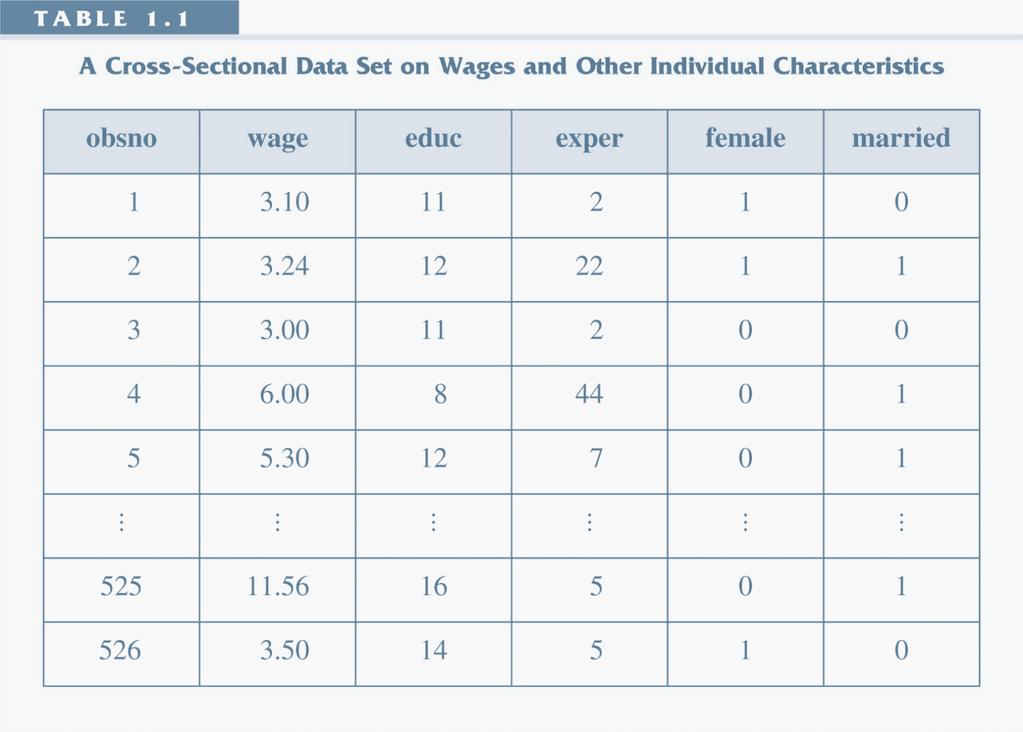
7 Cross-sectional Data 7 / 69

8 Time Series Data 8 / 69

9 Panel Data 9 / 69

10 Econometrics Observational data vs Experimental Data Experimental data: Experiment can control other variables, leaving only the one under study to di er across groups. Such data is easier to analyze. However, often we cannot conduct experiments, so we have to obtain the data as it is, called observational data. Then we need to control for variations due to other factors using statistical/ econometric techniques. Example: it is hard to randomly force people not to have education when they have a chance, so experiments are not feasible. So we have to depend on real-life data, where those who have the chance to have more education may be quite di erent from those who do not have the chance. Thus, some econometric tools are required. 10 / 69

11 Econometrics A typical econometric model: y i = f (x i, ε i ) y i is the dependent variable, which is the outcome variable of individual i (use t for time); x i is a vector of regressors, independent variables or explanatory variables, which explains the variations of y i. ε i is the disturbance/error, which represents the component that cannot be explained by the regressors. It is unobserved, and is the key stochastic component of the model. f is a function describing how x and ε a ect y. e.g. y: wage; x: education, age, gender, etc. 11 / 69

12 Econometrics x and f are mainly determined by theory, and f is also a ected by convenience in estimation and inference. The most fundamental functional form is the linear regression model y i = β 1 + x 2i β x ki β k + ε i, i = 1,..., n where β is a vector of parameters to be estimated. We will start with this model and the OLS approach, then discuss some complications when some basic assumptions are violated. Then, we will consider special approaches for speci c types of data (time series, panel data, binary dependent variables). 12 / 69

13 Procedure of an Econometric Analysis Determine your research question, understand related economic theory and collect data. Choose appropriate econometric models based on economic theory and nature of data. Mainly a Linear Regression Model for this class Determine what explanatory variables x should be included in the model, based on theory and data. Estimate the models using appropriate methods. If we suspect of some problems, reestimate the model in ways that can remedy the problems. Carry out speci cation tests if necessary. Interpret the parameter estimates of your model, perform hypothesis testing (related to economic theory) and answer the research question. Further analysis such as forecast or policy analysis. 13 / 69

14 Matrix algebra Notations of matrix (linear) algebra are used to shorten expressions. In case of no confusion, I do not bold vectors or matrices here. We usually work with column vectors, e.g. 0 1 x 1 x 2 x = B A x n We also call this an n 1 matrix. Sometimes we have row vectors, e.g. b = ( b 1 b 2 b n ) 14 / 69

15 Matrix algebra When we have two dimensions, we call it a matrix. 0 1 a 11 a 12 a 1n a 21 a 22 a 2n A = C. A a m1 a m2 a mn we call it an m n matrix. We call a matrix with just one element a scalar, where it is the same as a real number in usual context. The transpose of a matrix is formed by switching rows and columns. The transpose of A is denoted by A 0 (sometimes A T.) An element of the tranposed matrix a 0 ij = a ji. The dimension of A 0 is n m. Transpose of a column vector becomes a row vector. (AB) 0 = B 0 A 0 15 / 69

16 Matrix algebra Matrix addition / subtraction is just done element by element. Both matrices (or vectors) must have the same size. Multiplication of a scalar and a matrix: multiply the scalar to each element of the matrix. ((pa) ij = pa ij for a scalar p) Multiplcation of two matrices: For two matrices A np and B pm, AB is an n m matrix where the ij element is (AB) ij = p a ik b kj k=1 Note that AB 6= BA in general, even when they are both de ned and of the same size. Identity matrix I consists of 1 on the main diagonal and zero for other elements. For the identity matrix I and a square matrix A of the same size, IA = AI = A. 16 / 69

17 Matrix algebra Multiplication of two vectors: if a and b are column vectors of the same size n, then 0 1 a 1 b 1 a 1 b 2 a 1 b n a 0 n b = a j b j ; ab 0 a 2 b 1 a 2 b 2 a 2 b n = B C. A a n b 1 a n b 2 a n b n The former is a scalar. The latter is an n n matrix. Therefore x i1 β 1 + x 2i β x ki β k can be written as x 0 i β. So, for the same column vector a, a 0 a = n aj 2 j=1 which is sum of squares of the elements, and is always non-negative. 17 / 69

18 Matrix algebra If V is an n n square matrix, c is an n 1 column vector, then c 0 Vc is a scalar. If c 0 Vc > 0 for any non-zero vector c, we call V a positive de nite matrix. If c 0 Vc 0 for any vector c, we call V a positive semi-de nite matrix. Note: the diagonal elements of a positive de nite matrix must be positive. Why? A square matrix A is invertible or non-singular if its inverse A 1 exists, where A 1 A = AA 1 = I. (AB) 1 = B 1 A 1 if both A and B are square invertible matrices. A square matrix is invertible if it is of full rank, or any one of the column (row) cannot be expressed as a linear combination of other columns (rows). 18 / 69

19 Statistics Review A random variable (r.v.) takes a numerical value that corresponds to a certain set of random outcomes. As the outcome is random, the random variable is di erent for di erent realizations (draws from the distribution). It can be discrete, where it is possible to take nite or countable number of values. It can be continuous, where it can take any value on an interval. e.g. X = 1 if it rains tomorrow, X = 0 if it does not rain. e.g. X is the highest temperature of tomorrow. For practical purposes, we usually take r.v. as continuous in this class unless it mainly takes a small number of discrete values. 19 / 69

20 A Discrete Distribution 20 / 69

21 A Continuous Distribution 21 / 69

22 Statistics Review The distrbution function, or cumulative distribution function (cdf) of an r.v. X is F (x) = Pr(X x) The probability density function (pdf) of a continuous r.v. X is df (x) f (x) = dx So, the probability between a and b is Pr(a < X b) = Z b a f (x)dx = F (b) F (a) Note that for a continuous r.v., at each particular point, P(X = a) = 0 It is only meaningful to talk about the probability of an interval, say (a, b]. 22 / 69

23 Statistics Review The joint distribution of two random variables X and Y F (x, y) = Pr(X x, Y y) The corresponding density function is f (x, y) = 2 F x y Conditional distribution (density) f Y jx (yjx) = f (x, y) f X (x) so the joint density can be expressed as f (x, y) = f X (x)f Y jx (yjx) Two variables are statistically independent if f (x, y) = f X (x)f Y (y), 8x, y. 23 / 69

24 Statistics Review Expectation (general): a function g of an r.v. X, Z E (g(x )) = g(x)f (x)dx or g(x) Pr(X = x) Mean (First Moment) Z E (X ) = xf (x)dx or x Pr(X = x) = µ X Variance (Second Central Moment) Var(X ) = E (X E (X )) 2 = E (X 2 ) [E (X )] 2 = σ 2 X Skewness (Third Moment) E (X E (X )) 3 /σx 3 asymmetrical: two sides are not the same.) Kurtosis (Fourth Moment) E (X E (X )) 4 /σx 4 heavy tails) (non-zero if (large if 24 / 69

25 25 / 69

26 Covariance Statistics Review Cov(X, Y ) = E [(X E (X ))(Y E (Y ))] = σ XY This is a measure of linear relation between two variables. Correlation Cov(X, Y ) ρ XY = Corr(X, Y ) = p = σ XY Var(X )Var(Y ) σ X σ Y which lies between -1 and 1. If two variables always lie on an upward sloping straight line, then ρ XY = 1. If two variables always lie on a downward sloping straight line, then ρ XY = 1. If covariance/correlation are zero, X and Y are uncorrelated. Covariance/Correlation only measures linear relationship. There may be non-linear relationship that gives rise to zero correlation. 26 / 69

27 27 / 69

28 Statistics Review Conditional Expectation: The expectation of Y given the value of X. E (Y jx = x) = Z yf Y jx (yjx)dy or y Pr(Y = yjx = x) If there is some comovement between these variables, the above conditional distribution would change with x. Finding out how and by how much the conditional mean of Y varies with x is one of the important issues of this class. e.g E (wagejeduc). If the two random variables are independent, E (Y jx = x) = E (Y ) = µ Y. 28 / 69

29 29 / 69

30 Statistics Review Properties of Expectation E (ax + by ) = ae (X ) + be (Y ) Var(aX + by ) = a 2 Var(X ) + b 2 Var(Y ) + 2ab cov(x, Y ) By applying the above iteratively, addition of arbitrarily nite number of terms can be done similarly. More generally, E (ag(x ) + bh(y )) = ae (g(x )) + be (h(y )) However, the expectation cannot be passed into non-linear functions E (g(x )) 6= g(e (X )) 30 / 69

31 Statistics Review Linear function of random variables in matrix form Note that for a constant (column) vector a = (a 1,..., a K ) 0 and a random (column) vector x = (x 1,..., x K ) 0 which is a scalar. E (a 0 x) = E a 0 x = K a k x k k=1! K K a k x k = a k E (x k ) k=1 k=1 = a 0 E (x) = a 0 µ = K a k µ k k=1 31 / 69

32 Statistics Review Variance-Covariance Matrix Var(x) = E (x µ)(x µ) 0 = Σ So the (i, j) th element of the matrix is Σ ij = E [(x i µ i )(x j µ j )] = cov(x i, x j ) Σ ii = E (x i µ i ) 2 = var(x i ) Thus, the variance-covariance matrix of a vector of size K is a K K square matrix. The variance matrix is symmetric, and positive de nite. Outer product of the form E (u u 0 ) is the variance of a vector u (with E (u) = 0). Note the meaning of Σ: whether it means a variance matrix, or it means summation. Summation involves the range (i = 1,..., n), but we sometimes omit that. 32 / 69

33 Statistics Review For a linear combination in vector form, the variance is Var(a 0 x) = E (a 0 (x µ)(x µ) 0 a) = a 0 E [(x µ)(x µ) 0 ]a = a 0 Var(x)a = a 0 Σa where Σ = Var(X ) = E [(x µ)(x µ) 0 ] is the K K variance-covariance matrix of x. Σ is positive de nite implies the variance of the above linear combination of x must be positive. The above variance expression can be expressed in summation form: a 0 Σa = K k=1 a 2 k Var(x k ) + j,k;j6=k which agrees with what we have before. a j a k cov(x j x k ) 33 / 69

34 Statistics Review Consider a matrix A which consist of L rows of K-vectors: a a 11 a 12 a 1K 1 B C a 21 a 22 a 2K A A = C. A a L LK a L1 a L2 a LK An L-vector of linear combinations of elements in x is a 1 x K 1 j=1 a 1j x j B C B C Ax A A a L x K j=1 a Lj x j L1 Since a 1,..., a L are row vectors, we do not need to transpose. 34 / 69

35 Statistics Review So, which is a L 1 vector which is an L L matrix. E (Ax) = AE (x) = Aµ Var(Ax) = E (A(x µ)(x µ) 0 A 0 ) = AE ((x µ)(x µ) 0 )A 0 = AΣA 0 Remember, if the random vector is of dimension L, its variance matrix is L L. 35 / 69

36 A Few Common Distributions Statistics Review Normal Distribution: N(µ, σ 2 ) f (x) = p 1 (x µ) 2 exp 2πσ 2σ 2 When µ = 0, σ 2 = 1 (denoted as N(0, 1)), we call this a Standard Normal Distribution. Its density is in a bell shape, and symmetrical around the mean. If x N(µ, σ 2 ), then z = x µ σ N(0, 1) 36 / 69

37 37 / 69

38 Statistics Review A Few Common Distributions Chi-Square Distribution with degree of freedom p : χ 2 (p) It can be constructed by χ 2 = p Zi 2 i=1 where p is a positive integer, Z i N(0, 1) and Z i and Z j are independent. As it is a sum of squares, it always takes non-negative values. 38 / 69

39 39 / 69

40 A Few Common Distributions Statistics Review T distribution (Student s T distribution) with degree of freedom ν: T (ν) It can constructed by T = Z p P/ν where Z N(0, 1) and P χ 2 (ν) and Z, P are independent. It is like standard normal normal: bell-shaped and symmetric around zero, but it has a thicker tail (higher densities at two ends.) When v!, it converges to the Standard Normal Distribution. When ν > 100, it is practically close to a normal distribution. 40 / 69

41 41 / 69

42 A Few Common Distributions Statistics Review F Distribution with degrees of freedom p and q : F (p, q) It can be contructed by F = P/p Q/q where P χ 2 (p) and Q χ 2 (q) and P, Q are independent. As it is a ratio of two Chi-Square variables, it takes only non-negative values. When q!, Q/q! 1 and so, pf! P χ 2 (p). We will see how these distributions are useful in constructing statistical tests later on in this class. 42 / 69

43 43 / 69

44 Population and Sample Statistics Review Population is the world/ nature we want to learn about. Traditional view: it is known as all observations in the domain we investigate. (e.g. the population can be all people in a country, when we study the height, weight, wage distribution of a country.) Statistical view: data generating process: There is an underlying statistical distribution or model that generates each observation. Each observation is a realization of this data generating process. (e.g. each person s height is a draw from a height distribution, say with mean µ and variance σ 2. Or the wage is generated by a regression model.) It is the properties and relationship in the population that we want to know about. 44 / 69

45 Statistics Review We learn about our world through data. Very often we don t have all the data about the world (in the tranditional view), so we need to draw a sample from the population. A Sample is the part of the data we draw from the population to understand the world. (say obtaining the height of 100 people) From this sample, we want to estimate parameters (mean µ, β in regression model, etc) of the population and to test some hypotheses about the population. Because it is a random draw from the population, each sample would be di erent, and so are the statistics from the sample. 45 / 69

46 Statistics Review Consider we want to estimate the (population) mean µ of a certain variable. (e.g. the height of adult male) We denote the random variable X. Population Mean E (X ) = µ and Population Variance Var(X ) = σ 2. Assume a random sample is drawn from the population, which means each sample is an independent and identical distributed (iid) from the population. For each observation i, E (X i ) = µ and Var(X i ) = σ 2. A straightforward estimator for the mean µ is the sample mean X : X = 1 n n X i i=1 Since X i are random variables, X is also a random variable, and it takes di erent values from di erent samples. 46 / 69

47 Properties of the estimator Statistics Review E ( X ) = 1 n E (X i ) = 1 n nµ = µ Var( X ) = 1 n 2 Var(X i ) = 1 n nσ2 = σ2 n note that the covariance terms disappear, why? We usually looks for some good properties of an estimator. Unbiasedness: E ( X ) = µ. (Its expectation is at the true value of the parameter we want to estimate.) Consistency: When the sample size n goes to in nity, X n (sample mean of size n) converges in probability to the true mean µ. (Notation: X n! p µ.) It means when n becomes larger and larger, the distribution is denser and denser around the true value µ, and at the limit when n!, it collapses to the point µ. 47 / 69

48 48 / 69

49 Statistics Review A su cient condition for X n! p µ is that E ( X n ) = µ and Var( X n )! 0 as n!, which are clearly satis ed. An estimator is consistent if both are satis ed: 1. The distribution narrows down to a point (converges) when n goes to in nity; 2. This point is the true value. Inconsistent estimators: Example: only using the rst observation X 1 no matter how large the sample size is. Example: ( n i=1 1.2X i ) /n if µ 6= / 69

50 Statistics Review Law of Large Numbers (LLN) The most basic form is, if the sample X i are iid from the population with nite variance, then n 1 n X i! p E (X i ) i=1 So, sample mean converges in probability to population mean. As we can de ne another r.v. by letting Y i = g(x i ) for some continuous functions g, we have n 1 n g(x i )! p E (g(x i )) i=1 50 / 69

51 Statistics Review E ciency Recall that X as an estimator for µ, we have Var( X ) = σ 2 /n. The lower the variance of the estimator, the more likely the sample value to be closer to the true value. An estimator ˆθ is more e cient than another estimator eθ, given unbiased (or consistent) to θ, if Var( ˆθ) < Var(eθ) If it involves a vector of estimators, we replace the above inequality by D = Var(eθ) Var( ˆθ) is positive de nite. so that a 0 Da > 0 for any non-zero vector a, which means Var(a 0 eθ) Var(a 0 ˆθ) = a 0 Var(eθ)a a 0 Var( ˆθ)a > 0. So the variance of any linaer combination of ˆθ is smaller than the same linear combination with eθ. 51 / 69

52 Estimating Standard Error Statistics Review Recall Var( X ) = σ 2 /n. The standard deviation of the estimator is σ/ p n. However, we usually do not know σ 2 to start with. An unbiased and consistent estimator for σ 2 is the sample variance: s 2 = 1 n (X i X ) 2 n 1 i=1 It is divided by n 1 to adjust for the loss in one degree of freedom in estimating X. An (estimated) standard error is q s X = se( X ) = Var( \ X ) = r s 2 n = s p n 52 / 69

53 Statistics Review Sampling Distribution / Distribution of the Estimator The knowledge of the distribution of estimator is essential for us to perform hypothesis testing and construct con dence interval later in this section. Need to distinguish the cases where population is normally distributed or not. If the population is normally distributed so that X N(µ, σ 2 ), then by the property that linear combination of normally distributed random variables is still normal, we have! X n = 1 n n X i N(µ, σ2 i=1 n ) or p n( X n µ ) N(0, 1) σ However, we cannot use the above to justify the use of normal distribution if the population is not from a normal distribution. 53 / 69

54 Statistics Review Central Limit Theorem Luckily, we have a very amazing result about sample means. The Central Limit Theorem says that, if the observations X 1, X 2,..., X n drawn from the population are iid with nite variance, when the sample size n gets large, the sample mean X n would become closer and closer to a normal distribution, and at the limit when n!, it is exactly normally distributed, regardless of the population distribution. This is true even if the population itself is far from normal, say, uniform or binomial. 54 / 69

55 Samples from Bernolli distribution with P(X = 1) = 0.7. n = 2, 5, 10, 100 Density r(mean) Density r(mean) Density Density r(mean) r(mean) 55 / 69

56 Statistics Review Technically, we may use the notation of convergence in distribution. After normalization, Central Limit Theorem implies p n( X n µ)! d N(0, σ 2 ) or ( X n µ σ/ p n )!d N(0, 1) when X i are iid, regardless of the distribution of X i By making use of this, for a large but nite n, we can approximate the sampling distribution by X n app N(µ, σ2 n ) The resulting distribution is the same as the exact result for normal population, but it is an approximation for large sample if the population is not normal. For simple problems, a sample size of 30 is regarded as large. But, for more complicated problems, it is harder to say. 56 / 69

57 Statistics Review Similarly, for a vector of random variables. If we have an iid sample of K random variables, then p n( X n µ)! d N(0, Σ) where X n = 1 n n i=1 0 X 1i X 2i. X Ki 1 0 C A ; µ = µ 1 µ 2. µ K 1 C A and Σ is the variance matrix of the population variables (X 1,..., X K ) If a is a column vector of non-random scalars, then p n(a 0 X n a 0 µ)! d N(0, a 0 Σa) Q: What is the asy. distribution of X 1 X 2? 57 / 69

58 Statistics Review So, we know that if σ 2 is known, then z = X µ σ/ p n N(0, 1) It is exact if the population X follows normal distribution, and approximately true for large sample if the population is from other distribution. However, for most of the time, σ 2 is unknown. Consider the t-ratio t = X µ s/ p n = X µ se( X ) where we replace σ by the sample estimate s we introduced before. 58 / 69

59 Statistics Review When the population normally distributed, it can be shown that t = ( X µ)/(σ/ p n) q T (n 1) (n 1)( s 2 )/(n 1) σ 2 The numerator is distributed as standard normal, while the denominator can be shown to be the square root of a Chi-square random variable with degree of freedom (n 1) (i.e. χ 2 (n 1)) divided by (n 1). It can also be shown that these two are independent, and so by de nition t is Student-t distributed with degree of freedom (n 1). Notice that when n is large (e.g > 100), T and normal are close, so you may use normal distribution directly. This is true regardless of the sample size. 59 / 69

60 Statistics Review For non-normal population, we can (only) have asymptotic approximation: X µ p t = σ 2 /n p s 2 /σ 2 The numerator converges in distribution to N(0, 1), and the denominator converges in probability to 1, since s 2! p σ 2 and square root is a continuous function. Therefore t! d N(0, 1) So, for large enough sample, we have t approximately distributed as standard normal. We may also use T distribution if the sample size is between 30 to 100 as an approximation. This allows a thicker tail than the standard normal distribution. May directly use normal for n > / 69

61 Hypothesis Testing Statistics Review Besides the point estimate, say X, we may also like to test whether some belief (hypothesis) we have about the population is true or not. By making use of the knowledge about the distribution of the statistic (e.g. t above), we can perform hypothesis testing. We always talk about hypothesis about the population. Two-sided hypothesis: H 0 : µ = µ 0 vs H 1 : µ 6= µ 0 One-sided hypothesis: H 0 : µ = µ 0 vs H 1 : µ < (>)µ 0 The idea is that, if the null is true, and it is too extreme for the sample to show the X we see, then we have evidence that the null is not likely to be true. Otherwise, we don t have enough evidence that the null is false. 61 / 69

62 Statistics Review H 0 : µ = µ 0 H 1 : µ 6= µ 0 We use information of our sample, in particular X or the corresponding t, to judge whether the null is true. In this case, as X or t are approximately normally distributed, we do not have a region that X cannot take if the null is true. So, we have to allow for some errors. We choose α proportion of the distribution under the null (H 0 ) that is the most favorable to H 1, then we set this as the rejection region. α is the probability of Type I error (H 0 is true, but decide to reject H 0.) α is also commonly known as the signi cance level, or size of the test. 62 / 69

63 Statistics Review In this case, we make use of t = ( X µ 0 )/(s/ p n). If null is true, the the true mean is µ 0, and t is distributed as T (n 1). So, if X is so much away from µ 0 that jtj is so big that it lies on the most extreme α/2 area on either side (i.e. jtj > t α/2,n 1 ), then we reject the null (H 0 ). Otherwise, we cannot reject H 0. We don t have enough evidence that H 0 is false. We call t α/2,n 1 the critical value for the signi cance level α. Usually we use α = 5%. We sometimes use 10% or 1%. 63 / 69

64 Statistics Review Example: If we want to know about the height of female between the age in Shanghai. Suppose we have a random sample of the height of 100 female at this age. From the sample, X = 165.3, s 2 = 50.23, n = 100 We want to test the hypothesis that H 0 : µ = 162 vs. H 1 : µ 6= 162. T statistics is now t = p 50.23/100 = The critical value for 2-sided test at α = 5% is about 1.96 if using standard normal, and 1.99 if using T (99), so this is clearly too extreme, and so we can reject H 0 at 5% level. 64 / 69

65 Statistics Review Another way to make judgement is to use p-value. This is the probability of observing a statistic that is as or more extreme than what we have actually observed, given H 0 is true. If T n 1 T (n 1), then p = Pr(jT n 1 j jtj) = Pr(T n 1 jtj) + Pr(T n 1 jtj) where t is the t-ratio in the observed sample. The larger the p, the less extreme the sample is under null. Thus we reject when p is very small. The rule is to reject when p α. In the above example, p = Pr(jT 99 j 4.656) ' so we reject the null. Usually it is easier to obtain p-value through computer software. 65 / 69

66 Statistics Review For One-sided hypothesis: H 0 : µ = µ 0 vs H 1 : µ < (>)µ 0 The only di erence is that, we only reject if what we observe is on the side favorable to the alternative. If we use t-ratio, we need to adjust the critical value. If we use p-value, we only use the probability on the side favourable to the alternative. Example: if H 1 : µ > 162 instead, we use the critical value t α,n 1 = 1.66 (or z α = 1.645), and clearly we reject the null and we have evidence that it is larger than 162. p-value is now Pr(T ) ' Again, much smaller than α = 0.05, and so we reject the null hypothesis. What if the alternative is µ < 162? 66 / 69

67 Statistics Review There is also a Type II error, which is that given the H 1 is true, we fail to reject the null. Given we have limited data, there is a trade-o between Type I error against Type II error. If we want to reduce Type I error by making it harder to reject, it is also more likely to commit Type II error. If the standard error is large, it is hard to distinguish whether the null is indeed satis ed. e.g. If the standard error s for X is 10, it is di cult to distinguish whether it comes from a distribution with µ = 160 against µ = 165. The only way to reduce both types of errors is to reduce the standard error of your estimator, either by using your data more e ciently (a more e cient estimator) or to increase your sample size. (Recall se = s/ p n.) 67 / 69

68 Statistics Review We can also construct con dence interval for the population parameter µ using X and the related critical values. In 1 α proportion of the times the con dence interval constructed this way would include the true value µ. Pr( t α/2,n 1 < X µ s/ p n < t α/2,n 1) = 1 α rearranging, we have Pr( X t α/2,n 1 s p n < µ < X + t α/2,n 1 s p n ) = 1 This gives you an idea the likely range of the true parameter. If the (1 α) con dence interval does not include H 0, then the we reject the null of the test. Example: 95% con dence interval of the height of female is r ( 100 ) = (163.9, 166.7) 68 / 69 α

69 Statistics Review In this lecture we go through the statistical techniques we use to know about the population mean µ using X. We will do something similar, but concerning relations between variables. In this course, 1. We introduce the basic models and their underlying assumptions. 2. The method of estimation: Ordinary Least Squares (OLS) 3. Statistical Hypothesis Testing on parameters that represents economic relations. 4. What should be done if some basic assumptions are violated. 69 / 69