Richard Yung VEE regression analysis spring 2009 (510) Paid loss triangle: Parameter Stability.

Transcription

1 Richard Yung VEE regression analysis spring 9 (51) Paid loss triangle: Parameter Stability Introduction: As mentioned in the background description of the paid loss triangle, it is mainly affected by three factors: volume of business growth, inflation, and loss payment patterns. Regression analysis can use past or simulated data conveniently to estimate the coefficients of these three factors. Since business growth, inflation and loss payment patterns are very unlikely to remain constant from year to year; one must understand changes that are needed in regression analysis when any or all of these factors changed. In this project, regression analysis is used to generate residual plots of different simulations based on how inflation rate changes and which variables are regressed while volume of business growth and loss payment patterns of the regression equation are constant. Simulated random errors were also introduced to see if the generated residual plots will reflect how the calculated regression equations are affected by stochasticity. Simulation Setup: A VBA macro MS Excel was written in a way to simulate paid loss triangle, perform regression analysis using its Data Analysis Toolpak, and generate residual plots against development and calendar. The macro utilized parameters entered in the worksheet named parameters and simulates 5 scenarios: Simulation 1: constant inflation rate with CY and DY regressed Simulation : discretely changed inflation rate with only CY and DY regressed Simulation 3: discretely changed inflation rate with all variables regressed Simulation 4: continuously changed inflation rate with only CY and DY regressed Simulation 5: continuously changed inflation rate with all variables regressed The only difference of parameter usage is that β b was used as the final inflation rate in simulation 4 and 5. Consequently, β continuously shifted towards β b at a constant rate each consecutive year. The rate of change was calculated from β, β b, and the year when inflation rate started to change. The parameters names and the method of simulating errors were the same ones listed in illustrative worksheet provided by NEAS. In this project, different levels of stochasticity via different values of σ were tested in all simulations. Also, the -test method was used to compare simulations and 3 and simulations 4 and 5. Proposed Equations: In order to test if a proposed regression equation fits well, sigma is set to in the simulations. Since simulation 1 assumes all parameters (α, β 1, β, are constant), the proposed equation is E ( Y ) = α + β1( DY) + β ( CY ) + ε. Simulation and 3, on the contrary have to use a modified equation from simulation 1 because of the changed inflation rate. By using a dummy variable and introducing another variable k, where the

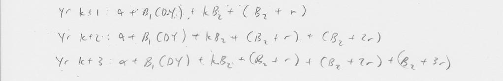
2 end of k th year is when inflation rate changed. Thus, the E(Y) should be equations: E Y ) = α + β ( DY ) + β ( k) + β b ( CY ) + ε when inflation rate changed, and ( 1 k ( Y ) = α + β1( DY) + β ( CY ) + ε E before the inflation rate changed. Simulation 4 and 5 also use a modified equation from simulation 1 also because of the changed inflation rate. However, the inflation rate is changed continuously instead. Another estimator β a and variable k are introduced here as well. Let r be the continuous rate of inflation rate change and k is where the end of k th year is when inflation rate β b β changed. Thus, β a =.Thus the E(Y) should be equations: CY k ( CY k)( CY k+ 1) E( Y ) = α + β1( DY ) + β ( CY ) + β a + ε when inflation rate changed, and E ( Y ) = α + β1( DY) + β ( CY ) + ε before the inflation rate changed. (See appendix for the derivations of these equations) Results of 1 st Simulation Run: The importance of this run was that all simulations used the very same low sigma of.1, thus testing the accuracy of each simulation. The other parameters were also the same in each simulation. Parameters for Run #1: Sigma.1 Alpha 15 beta beta.5 beta1b -.15 betab. CY DY x th year inflation changed? 1 betaa.1875 Simulation 1:

3 CY residuals: Simulation 1 statistics: Multiple R R Square Square.9997 Error.1675 Observations 1 df SS MS Regression Residual Total Coefficients Error t Stat P-value Lower Alpha Beta Beta E As expected, the adjusted R is approximately 1, the standard error is close to.1, and the coefficient α, β 1, β, were also very close to their respective inputted values. of -stat is, indicating that hypothesis of β 1, β are can be rejected. The plotted against calendar showed a relatively horizontal line proving that the equation E ( Y ) = α + β1( DY) + β ( CY ) + ε is a very good fit if the coefficients are assumed to be constant throughout the development and calendar.

4 Simulation : CY residuals: Simulation statistics: SUMMARY OUTPUT Multiple R R Square Square Error.1931 Observations 1 df SS MS Regression E-118 Residual Total

5 Coefficients Error t Stat P-value Lower Alpha E Beta E Beta E The adjusted R and the standard error were calculated to around.93 and.19 respectively. urthermore, even though the coefficient α and β 1 are close to the respective inputted values, β was found to be no where near.5. The plotted against calendar showed a V shape, proving that the equation E ( Y ) = α + β1( DY) + β ( CY ) + ε was not a good fit for a linear model. Simulation 3: CY residuals: E E

6 Simulation 3 statistics: Multiple R R Square Square Error.974 Observations 1 Df SS MS Regression Residual E-5 Total Coefficients Error t Stat P-value Lower Alpha Beta Beta E Betab By including an extra variable which indicated the year when inflation rate changed in this regression analysis, the adjusted R became very close to 1, and the coefficient α, β 1, β, and β b were also very close to their respective inputted values. -test would be used to compare simulation and 3. Since simulation s regression equation was E( Y ) = α + β1( DY) + β ( CY ) + ε and simulation 3 s regression is E( Y ) = α + β1( DY ) + β ( k) + β b ( CY k) + ε, simulation s regression equation would be restricted and simulation 3 s regression equation would be unrestricted. So - test would be: ( RUR RR ) / q ( ) /1 q, k = 1,1 3 = (1 R ) /( k) ( ) /(1 3) UR The -test statistic was greater than the critical values for 1,1 3 between 3.9 and 3.84 for 5% significance, and between 6.85 and 6.63 for 1% significance. Either way, this showed that variable k introduced in simulation 3 was statistically significant.

7 Simulation 4: CY residuals: Simulation 4 statistics: Multiple R R Square Square Error Observations 1 df SS MS Regression E-145 Residual Total

8 Coefficients Error t Stat P-value Lower Alpha Beta E Beta E The adjusted R and the standard error were calculated to around.95 and.13 respectively. Also, only the coefficient β 1 are close to the respective inputted value. α was found to be and β was found to be near.9. The plotted against calendar showed a rounded v shape, proving that the equation E ( Y ) = α + β1( DY ) + β ( CY ) + ε was not a good fit for a linear regression model. Simulation 5: CY residuals:

9 Simulation 5 statistics: Multiple R R Square Square Error.14 Observations 1 df SS MS Regression Residual Total Coefficients Error t Stat P-value Lower Alpha Beta E- Beta E- Betaa Just like simulation 3, by including an extra variable which indicated the year when inflation rate changed in this regression analysis, the adjusted R became very close to 1, and the coefficient α, β 1, β, and β b were also very close to their respective inputted values. -test would also be used to compare simulation 4 and 5. Since simulation 4 s regression equation was E( Y ) = α + β1( DY) + β ( CY ) + ε and simulation 5 s regression ( CY k)( CY k+ 1) equation was E( Y ) = α + β1( DY ) + β ( CY ) + β a + ε, simulation 4 s regression equation would be restricted and simulation 5 s regression equation would be unrestricted. So -test would be: ( RUR RR ) / q ( ) /1 q, k = 1,1 3 = (1 R ) /( k) ( ) /(1 3) UR The -test statistic was greater than the critical values for 1,1 3 between 3.9 and 3.84 for 5% significance, and between 6.85 and 6.63 for 1% significance. Either way, this showed that variable k introduced in simulation 5 was statistically significant. Results of nd Simulation Run: After using low stochasticity to find out the accuracies and patterns of the five simulations, a larger value of sigma could be used to see if the same patterns would be masked by stochasticity in each of the simulations. This run was that all simulations used a higher sigma of.5. The other parameters were also the same as the ones in previous each simulation run.

10 Parameters for Run #: Sigma.5 Alpha 15 beta beta.5 beta1b -.15 betab. CY DY x th year inflation changed? 1 betaa.1875 Simulation 1: CY residuals: Simulation 1 statistics: Multiple R R Square.8871 Square Error.4661 Observations 1

11 df SS MS Regression E-99 Residual Total Coefficients Error t Stat P-value Lower Alpha E Beta E Beta E Because of the larger error values due to higher sigma, the adjusted R is now approximately.89 and the standard error is about.4. Similarly, the coefficient α, β 1, β also deviated slightly from their respective inputted values. The plotted against calendar also showed a noisier horizontal line, proving that it was affected by higher value of sigma. Simulation : CY residuals:

12 Simulation statistics: Multiple R R Square Square Error.9381 Observations 1 df SS MS Regression E-86 Residual Total Coefficients Error t Stat P-value Lower Alpha E Beta E Beta E Unlike previous simulation, the adjusted R dropped to.85 and the standard error increased to.9. Not only that, the coefficients α, and β 1 also drifted slightly away from their respective inputted values. The plotted against calendar showed a V shape,, but it was not a perfect V shape as seen in run 1 simulation. Thus, this also showed that the regression was affected by higher value of sigma. Simulation 3:

13 CY residuals: Simulation 3 statistics: Multiple R R Square.8888 Square Error Observations 1 df SS MS Regression E-94 Residual Total Coefficients Error t Stat P-value Lower Alpha E Beta E Beta E Betab E As noted earlier, this was the more accurate regression of discretely changed inflation rate. The adjusted R was.88 opposed to.85 from previous simulation. Just like the previous run, -test would be used to compare simulation and 3, which is: ( RUR RR ) / q ( ) /1 q, k = 1,1 3 = (1 RUR ) /( k) (1.8888) /(1 3) The -test statistic was a lot smaller than the one calculated previously, but it was still greater than the critical values for 1,1 3 between 3.9 and 3.84 for 5% significance, and between 6.85 and 6.63 for 1% significance. Either way, this showed that variable k introduced in simulation 3 was still statistically significant. Also, just like -test statistic, the residuals plot against calendar showed that the seemingly horizontal line was affected more by higher value of sigma.

14 Simulation 4: CY residuals: Simulation 4 statistics: Multiple R R Square Square Error Observations 1 df SS MS Regression E-81 Residual Total

15 Coefficients Error t Stat P-value Lower Alpha E Beta E Beta E The adjusted R was.83 and the standard error was.8. The plotted against calendar showed a rounded, but noisier V shape, unlike the one seen in run 1 simulation 4. Thus, this showed that the regression was affected by the higher value of sigma. Simulation 5: CY residuals:

16 Simulation 5 statistics: Multiple R.9957 R Square Square Error.437 Observations 1 df SS MS Regression E-88 Residual Total Coefficients Error t Stat P-value Lower Alpha E Beta E Beta E Betaa E Also noted earlier, this was the more accurate regression of continuously changed inflation rate. The adjusted R was.86 opposed to.83 from previous simulation. -test would also be used to compare simulation 4 and 5, which would be: ( RUR RR ) / q ( ) /1 q, k = 1,1 3 = (1 RUR ) /( k) ( ) /(1 3) The -test statistic was a lot smaller than the one calculated previously, but it was still greater than the critical values for 1,1 3 between 3.9 and 3.84 for 5% significance, and between 6.85 and 6.63 for 1% significance. Either way, this showed that variable k introduced in simulation 5 was still statistically significant. Also, just like -test statistic, the residuals plot against calendar showed that the seemingly horizontal line was affected more by the higher value of sigma. Results of 3 rd Simulation Run: Previously, a moderate value of sigma was used to find out that the simulated random errors were not large enough to mask the significance of new variables introduced in simulation 3 and 5. Now, a larger value of sigma would be used to see if the same patterns would show in each of the simulations. This run was that all simulations used an even higher sigma of.6. The other parameters were also the same as the ones in previous each simulation run.

17 Parameters for Run #3: Sigma.6 Alpha 15 beta beta.5 beta1b -.15 betab. CY DY x th year inflation changed? 1 betaa.1875 Simulation 1: CV Residuals: Simulation 1 statistics: Multiple R R Square Square Error Observations 1

18 df SS MS Regression E-4 Residual Total Coefficients Error t Stat P-value Lower Alpha E Beta E Beta E Since an even higher sigma was used, the adjusted R is now approximately.59 and the standard error is about.55. The plotted against calendar also showed a higher absolute residual averages, proving that it was affected by the higher value of sigma. Simulation : CV Residuals:

19 Simulation statistics: Multiple R R Square Square.6186 Error.5557 Observations 1 df SS MS Regression E-43 Residual Total Coefficients Error t Stat P-value Lower Alpha E Beta E Beta E Just as the sigma increased, the adjusted R dropped even lower to.61 and the standard error increased to.55. urthermore, it was harder to tell whether the average residuals plotted against calendar showed a V shape, or a noisy horizontal trend as in simulation 1. Therefore, this also showed that the regression was affected by the higher value of sigma. Simulation 3:

20 CV Residuals: Simulation 3 statistics: Multiple R R Square Square Error.5964 Observations 1 df SS MS Regression E-36 Residual Total Coefficients Error t Stat P-value Lower Alpha E Beta E Beta Betab E The adjusted R was.55 opposed to.61 from simulation and the standard error was.6. Just like the previous runs, -test would be used to compare simulation and 3, which is: ( RUR RR ) / q ( ) /1 q, k = 1,1 3 = 8.84 (1 R ) /( k) ( ) /(1 3) UR The -test statistic was less than the critical values for 1,1 3 between 3.9 and 3.84 for 5% significance, and between 6.85 and 6.63 for 1% significance. The introduced variable k in simulation 3 was no longer statistically significant. Also, it was much more difficult to tell if the residuals plot against calendar showed even a seemingly horizontal line. Both these pointed out that stochasticity was large enough to mask the significance of the newly introduced variable.

21 Simulation 4: CV Residuals: Simulation 4 statistics: Multiple R.787 R Square Square Error Observations 1 df SS MS Regression E-3 Residual Total

22 Coefficients Error t Stat P-value Lower Alpha E Beta E Beta E The adjusted R was.5 and the standard error was.6. The difference here was that the plotted against calendar did not show a V shape. This showed that the V shape of the regression had less impact than the stochasticity introduced in this simulation. Simulation 5: CV Residuals:

23 Simulation 5 statistics: Multiple R R Square Square.5611 Error.651 Observations 1 df SS MS Regression E-3 Residual Total Coefficients Error t Stat P-value Lower Alpha E Beta E Beta E Betaa The adjusted R was.51 opposed to.5 from simulation 4 and the standard error was.6. Just like the previous runs, -test would be used to compare simulation 4 and 5, which is: ( RUR RR ) / q ( ) /1 q, k = 1,1 3 = (1 R ) /( k) ( ) /(1 3) UR The -test statistic was greater than the critical values for 1,1 3 between 3.9 and 3.84 for 5% significance, but less than the range between 6.85 and 6.63 for 1% significance. The introduced variable k in simulation 5 was statistically significant enough at level of confidence. Also, it was much more difficult to tell if the residuals plot against calendar showed even a seemingly horizontal line. These also pointed out that stochasticity was large enough to mask the significance of the newly introduced variable. Conclusion: These simulations have shown that when a change in the inflation rate was introduced in the paid loss triangle simulation, two factors would affect the regression analysis: the inclusion of the extra variable being the year when the change occurred, and the severity of stochasticity affecting the data points. As long as the effect of stochasticity was small enough, the regression equation including the extra variable would be the better fit.

24 Appendix:

25