Electromagnetic Wave Propagation Lecture 2: Uniform plane waves
|
|
|
- Wesley Bruce
- 6 years ago
- Views:
Transcription

1 Electromagnetic Wave Propagation Lecture 2: Uniform plane waves Daniel Sjöberg Department of Electrical and Information Technology March 25, 2010
2 Outline 1 Plane waves in lossless media General time dependence Time harmonic waves 2 Polarization 3 Propagation in lossy media 4 Oblique propagation and complex waves 5 Paraxial approximation: beams 6 Doppler effect and negative index media 7 Conclusions
3 Outline 1 Plane waves in lossless media General time dependence Time harmonic waves 2 Polarization 3 Propagation in lossy media 4 Oblique propagation and complex waves 5 Paraxial approximation: beams 6 Doppler effect and negative index media 7 Conclusions
4 Plane electromagnetic waves In this lecture, we dive a bit deeper into the familiar right-hand rule. This is the building block for most of the course.
5 Outline 1 Plane waves in lossless media General time dependence Time harmonic waves 2 Polarization 3 Propagation in lossy media 4 Oblique propagation and complex waves 5 Paraxial approximation: beams 6 Doppler effect and negative index media 7 Conclusions
6 Propagation in source free, isotropic, non-dispersive media The electromagnetic field is assumed to depend only on one coordinate, z. This implies and by using ẑ z E = B t H = D t D = 0 B = 0 E(x, y, z, t) = E(z, t) D(x, y, z, t) = ɛe(z, t) H(x, y, z, t) = H(z, t) B(x, y, z, t) = µh(z, t) we have ẑ E z = µ H t = ẑ H z = ɛ E t E z z = 0 E z = 0 H z z = 0 H z = 0
7 Rewriting the equations The electromagnetic field has only x and y components, and satisfy ẑ E z = µ H t ẑ H z = ɛ E t Using (ẑ F ) ẑ = F for any vector F orthogonal to ẑ, and c = 1/ ɛµ and η = µ/ɛ, we can write this as (ηh ẑ) t z E = 1 c z (ηh ẑ) = 1 c which is a symmetric hyperbolic system ( ) E = 1 ( 0 1 z ηh ẑ c t 1 0 t E ) ( ) E ηh ẑ
8 Wave splitting We could eliminate the magnetic field to find the wave equation ( 2 z ) c 2 t 2 E(z, t) = 0 but it is often more convenient to keep the system formulation. The change of variables ( ) E+ = 1 ( ) E + ηh ẑ = 1 ( ) ( ) 1 1 E 2 E ηh ẑ ηh ẑ E is called a wave splitting and diagonalizes the system to E + z E z = 1 E + c t = + 1 E c t E + (z, t) = F (z ct) E (z, t) = G(z + ct)
9 Forward and backward waves The total fields can now be written E(z, t) = F (z ct) + G(z + ct) H(z, t) = 1 ) (F η ẑ (z ct) G(z + ct) A graphical interpretation of the forward and backward waves is
10 Energy density in one single wave A wave propagating in positive z direction satisfies H = 1 η ẑ E x: Electric field y: Magnetic field z: Propagation direction The Poynting vector and energy densities are (using the BAC-CAB rule A (B C) = B(A C) C(A B)) P = E H = 1 η E (ẑ E) = 1 η ẑ E 2 w e = 1 2 ɛ E 2 w m = 1 2 µ H 2 = 1 2 µ 1 η 2 ẑ E 2 = 1 2 ɛ E 2 = w e The transport velocity of electromagnetic energy is then P v = = 1 w e + w m η ẑ 1 ɛ = cẑ
11 Energy density in forward and backward wave If the wave propagates in negative z direction, we have H = 1 η ( ẑ) E and P = E H = 1 η E ( ẑ E) = 1 η ẑ E 2 Thus, when the wave consists of one forward wave F (z ct) and one backward wave G(z + ct), we have P = E H = 1 ( F η ẑ 2 G 2) w = 1 2 ɛ E µ H 2 = ɛ F 2 + ɛ G 2
12 Generalization for nonlinear media: simple waves A generalization of the plane wave concept is to look for solutions depending only on a scalar function of space and time E(x, y, z, t) = E(ϕ(x, y, z, t)) (linear media: ϕ = z ct) This can help analyze nonlinear material models with instantaneous response (for instance a Kerr model D = ɛ 0 (E + α E 2 E)) D(x, y, z, t) = D(E(x, y, z, t)) Maxwell s equations can then be written ϕ E = ϕ B t H H ϕ H = ϕ D t E E
13 Simple waves, continued The wavefronts and wave slowness are defined by ϕ(x, y, z, t) = constant s = ϕ (unit s/m) ϕ t Maxwell s equations become a symmetric algebraic problem ( ) ( 0 s I E ) ( D ) ( s I 0 H = E 0 E ) B 0 H H where D B E = ɛ(e) is the differential permittivity and H = µ(h) is the differential permeability. The eigenvalue s (and hence propagation speed) depends on field strengths E and H.
14 Shock waves Initial data propagate with a speed depending on field strength. Rarefaction wave Fast wave outruns the slow wave Shock wave Fast wave overtakes the slow wave
15 Outline 1 Plane waves in lossless media General time dependence Time harmonic waves 2 Polarization 3 Propagation in lossy media 4 Oblique propagation and complex waves 5 Paraxial approximation: beams 6 Doppler effect and negative index media 7 Conclusions
16 Time harmonic waves We assume harmonic time dependence E(x, y, z, t) = E(z)e jωt H(x, y, z, t) = H(z)e jωt Using the same wave splitting as before implies E ± z = 1 c E ± t = jω c E ± E ± (z) = E 0± e jkz where k = ω/c is the wave number in the medium. Thus, the general solution for time harmonic waves is E(z) = E 0+ e jkz + E 0 e jkz H(z) = H 0+ e jkz + H 0 e jkz = 1 η ẑ ( E 0+ e jkz E 0 e jkz) The triples {E 0+, H 0+, ẑ} and {E 0, H 0, ẑ} are right-handed systems.
.")
17 Wavelength A time harmonic wave propagating in the forward z direction has the space-time dependence E(z, t) = E 0+ e j(ωt kz) and H(z, t) = 1 η ẑ E(z, t). The wavelength corresponds to the spatial periodicity according to e jk(z+λ) = e jkz, meaning kλ = 2π or λ = 2π k = 2πc ω = c f
18 Refractive index The wavelength is often compared to the corresponding wavelength in vacuum λ 0 = c 0 f The refractive index is n = λ 0 λ = k = c 0 ɛµ k 0 c = ɛ 0 µ 0 Important special case: non-magnetic media, where µ = µ 0 and n = ɛ/ɛ 0. c = c 0 n, η = η 0 n, }{{} only for µ = µ 0! λ = λ 0 n, k = nk 0 Note: We use c 0 for the speed of light in vacuum and c for the speed of light in a medium, even though c is the standard for the speed of light in vacuum!
19 Energy density and power flow For the general time harmonic solution E(z) = E 0+ e jkz + E 0 e jkz H(z) = 1 η ẑ ( E 0+ e jkz E 0 e jkz) the energy density and Poynting vector are w = 1 ] [ɛe(z) 4 Re E (z) + µh(z) H (z) = 1 2 ɛ E ɛ E 0 2 P = 1 ] ( 1 [E(z) 2 Re H (z) = ẑ 2η E ) 2η E 0 2
20 Wave impedance For forward and backward waves, the impedance η = µ/ɛ relates the electric and magnetic field strengths to each other. E ± = ±ηh ± ẑ When both forward and backward waves are present this is generalized as (in component form) Z x (z) = Z y (z) = [E(z)] x = E x(z) [H(z) ẑ] x H y (z) = η E 0+xe jkz + E 0 x e jkz E 0+x e jkz E 0 x e jkz [E(z)] y = E y(z) [H(z) ẑ] y H x (z) = η E 0+ye jkz + E 0 y e jkz E 0+y e jkz E 0 y e jkz Thus, the wave impedance is in general a non-trivial function of z. This will be used as a means of analysis and design in the course.
21 Material and wave parameters We note that we have two material parameters Permittivity ɛ, defined by D = ɛe. Permeability µ, defined by B = µh. But the waves are described by the wave parameters Wave number k, defined by k = ω ɛµ. Wave impedance η, defined by η = µ/ɛ. This means that in a scattering experiment, we primarily get information on k and η, not ɛ and µ. In order to get material data, a theoretical material model must be applied. Often, wave number is given by transmission data (phase delay), and wave impedance is given by reflection data (impedance mismatch). More on this in future lectures!
22 Outline 1 Plane waves in lossless media General time dependence Time harmonic waves 2 Polarization 3 Propagation in lossy media 4 Oblique propagation and complex waves 5 Paraxial approximation: beams 6 Doppler effect and negative index media 7 Conclusions
23 Why care about different polarizations? Different materials react differently to different polarizations. Linear polarization is sometimes not the most natural. For propagation through the ionosphere (to satellites), or through magnetized media, often circular polarization is natural.
24 Complex vectors The time dependence of the electric field is E(t) = Re{E 0 e jωt } where the complex amplitude can be written E 0 = ˆxE 0x + ŷe 0y + ẑe 0z = ˆx E 0x e jα + ŷ E 0y e jβ + ẑ E 0z e jγ where E 0r and E 0i are real-valued vectors. We then have = E 0r + je 0i E(t) = Re{(E 0r + je 0i )e jωt } = E 0r cos(ωt) E 0i sin(ωt) This lies in a plane with normal ˆn = ± E 0r E 0i E 0r E 0i
25 Linear polarization The simplest case is given by E 0i = 0, implying E(t) = E 0r cos ωt. y E 0r x
26 Circular polarization Assume E 0r = ˆx and E 0i = ŷ. The total field E(t) = ˆx cos ωt + ŷ sin ωt then rotates in the xy-plane: y x E(t) The rotation direction needs to be compared to the propagation direction.
27 Circular polarization and propagation direction
28 Elliptical polarization The general polarization is elliptical The direction ê is parallel to the Poynting vector (the power flow).
29 Classification of polarization The following classification can be given: jê (E 0 E 0) Polarization = 0 Linear polarization > 0 Right handed elliptic polarization < 0 Left handed elliptic polarization Further, circular polarization is characterized by E 0 E 0 = 0. Typical examples: Linear: E 0 = ˆx or E 0 = ŷ. Circular: E 0 = ˆx jŷ (right handed) or E 0 = ˆx + jŷ (left handed). See the literature for more in depth descriptions.
30 Alternative bases in the plane To describe an arbitrary vector in the xy-plane, the unit vectors ˆx and ŷ are usually used. However, we could just as well use the RCP and LCP vectors ˆx jŷ and ˆx + jŷ Sometimes the linear basis is preferrable, sometimes the circular.
31 Outline 1 Plane waves in lossless media General time dependence Time harmonic waves 2 Polarization 3 Propagation in lossy media 4 Oblique propagation and complex waves 5 Paraxial approximation: beams 6 Doppler effect and negative index media 7 Conclusions
32 Lossy media We study lossy isotropic media, where D = ɛ d E, J = σe, B = µh The conductivity is incorporated in the permittivity, ( J tot = J + jωd = (σ + jωɛ d )E = jω ɛ d + σ ) E jω which implies a complex permittivity ɛ c = ɛ d j σ ω Often, the dielectric permittivity ɛ d is itself complex, ɛ d = ɛ d jɛ d.
33 Examples of lossy media Metals (high conductivity) Liquid solutions (ionic conductivity) Resonant media Just about anything!
34 Characterization of lossy media In the previous lecture, we have shown that a passive material is characterized by [ ( )] ɛ ξ Re jω 0 ζ µ For isotropic media with ɛ = ɛ c I, ξ = ζ = 0 and µ = µ c I, this boils down to ɛ c = ɛ c jɛ c µ c = µ c jµ c ɛ c 0 µ c 0
35 Maxwell s equations in lossy media Assuming dependence only on z we obtain { E = jωµc H z ẑ E = jωµ ch H = jωɛ c E z ẑ H = jωɛ ce Nothing really changes compared to the lossless case, for instance it is seen that the fields do not have a z-component. This can be written as a system ( E ) z η c H ẑ = ( ) ( ) 0 jkc E jk c 0 η c H ẑ where the complex wave number k c and the complex wave impedance η c are k c = ω ɛ c µ c, and η c = µc ɛ c
36 The parameters in the complex plane The parameters ɛ c, µ c, and k c = ω ɛ c µ c take their values in the complex lower half plane, whereas η c = µ c /ɛ c is restricted to the right half plane. ÁÑ Ê ÁÑ Ê
37 Solutions The solution to the system ( ) ( ) ( ) E 0 jkc E = z η c H ẑ jk c 0 η c H ẑ can be written (no z-components in the amplitudes E + and E ) E(z) = E + e jkcz + E e jkcz H(z) = 1 ẑ (E + e jkcz E e jkcz) η c Thus, the solutions are the same as in the lossless case, as long as we complexify the coefficients.
38 Exponential damping The dominating effect of wave propagation in lossy media is exponential damping of the amplitude of the wave: k c = β jα e jkcz = e jβz e αz Thus, α = Im(k c ) represents the damping of the wave, whereas β = Re(k c ) represents the oscillations. The exponential is sometimes written in terms of γ = jk c = α + jβ as e γz = e jβz e αz where γ corresponds to a spatial Laplace transform variable, in the same way that the temporal Laplace variable is s = jω + ν.
39 Poynting s theorem Poynting s theorem for isotropic media (ɛ c = ɛ c jɛ c and µ c = µ c jµ c) is 1 2 Re{E H } = ω ( ɛ 2 c E 2 + µ c H 2) We will write out the left and right hand side explicitly to see if they are indeed equal.
40 The Poynting vector Consider a wave propagating in the positive z direction, E(z) = E 0 e jkcz The Poynting vector is H(z) = 1 ẑ E 0 e jkcz η c 1 2 Re{E(z) H(z) } = 1 { 2 Re E 0 (ẑ E 0) 1 } ηc e jβz αz+jβz αz with the divergence = ẑ 1 2 Re( 1 ηc ) E 0 2 e 2αz 1 2 Re{E H } = 1 2 z Re( 1 ηc ) E 0 2 e 2αz = α Re( 1 ηc ) E 0 2 e 2αz
41 Material losses For the plane wave under study we have H = 1 η c ẑ E 0 e jβz αz, which implies ω 2 H 2 = 1 η c 2 E 0 2 e 2αz = ɛ c µ c E 0 2 e 2αz The right hand side of Poynting s theorem is then ( ɛ c ɛ c ( ɛ c E 2 + µ c H 2) = ω 2 c + µ µ c ) E 0 2 e 2αz
42 Poynting s theorem In order for Poynting s theorem to be satisfied, this requires α Re( 1 ηc ) = ω ( ) ɛ c + µ c ɛ c 2 µ c This is not a trivial relation to prove. In the case of non-magnetic media (µ c = µ 0, α = ω Im( ɛ c µ 0 ), 1/η c = ɛ c /µ 0 ), the explicit form is Im( ɛ c ) Re( ɛ c ) = 1 2 ɛ c = 1 2 Im(ɛ c) This is true due to the general relation (valid for any complex number w) Im(w 2 ) = 2 Re(w) Im(w)
43 Poynting s theorem In conclusion, Poynting s theorem 1 2 Re{E H } = ω ( ɛ 2 c E 2 + µ c H 2) is valid for waves propagating in lossy media, but the equality is obscured by some complex algebra.
44 Characterization of attenuation The power is damped by a factor e 2αz. The attenuation is often expressed in logarithmic scale, decibel (db). A = e 2αz A db = 10 log 10 (A) = 20 log 10 (e)αz = 8.686αz Thus, the attenuation coefficient α can be expressed in db per meter as α db = 8.686α Instead of the attenuation coefficient, often the skin depth (also called penetration depth) δ = 1/α is used. When the wave propagates the distance δ, its power is attenuated a factor e 2 7.4, or db 9 db.
45 Characterization of losses A common way to characterize losses is by the loss tangent (sometimes denoted tan δ) tan θ = ɛ c ɛ c = ɛ d + σ/ω ɛ d which usually depends on frequency. In spite of this, it is often seen that the loss tangent is given for only one frequency. This may be acceptable if the material properties vary little with frequency.
46 Example of material properties From D. M. Pozar, Microwave Engineering: Material Frequency ɛ r tan θ Beeswax 10 GHz Fused quartz 10 GHz Gallium arsenide 10 GHz Glass (pyrex) 3 GHz Plexiglass 3 GHz Silicon 10 GHz Styrofoam 3 GHz Water (distilled) 3 GHz
47 Approximations for weak losses In weakly lossy dielectrics, the material parameters are (where ɛ c ɛ c) ɛ c = ɛ c jɛ c = ɛ c(1 j tan θ) µ c = µ 0 The wave parameters can then be approximated as k c = ω ɛ c µ c ω ( ɛ cµ 0 1 j 1 ) 2 tan θ µc µ0 η c = (1 ɛ c ɛ + j 12 ) tan θ c If the losses are caused mainly by a small conductivity, we have ɛ c = σ/ω, tan θ = σ/(ωɛ c), and the attenuation constant α = Im(k c ) = 1 2 ω ɛ cµ 0 σ ωɛ c = σ 2 µ0 is proportional to conductivity and independent of frequency. ɛ c
48 Example: propagation in sea water A simple model of the dielectric properties of sea water is ( ɛ c = ɛ 0 81 j 4 S/m ) ωɛ 0 that is, it has a relative permittivity of 81 and a conductivity of σ = 4 S/m. The imaginary part is much smaller than the real part for frequencies f 4 S/m = 888 MHz 81 2πɛ 0 for which we have α = 728 db/m. For lower frequencies, the exact calculations give f = 50 Hz α = db/m δ = 35.6 m f = 1 khz α = 1.09 db/m δ = 7.96 m f = 1 MHz α = db/m δ = cm f = 1 GHz α = db/m δ = 1.29 cm
49 Approximations for good conductors In good conductors, the material parameters are (where σ ωɛ) ( ɛ c = ɛ jσ/ω = ɛ 1 j σ ) ωɛ µ c = µ The wave parameters can then be approximated as k c = ω ɛ c µ c ω j σ ωµσ ω µ = (1 j) 2 µc µ ωµ η c = ɛ c jσ/ω = (1 + j) 2σ This demonstrates that the wave number is proportional to ω rather than ω in a good conductor, and that the real and imaginary part have equal amplitude.
50 Skin depth The skin depth of a good conductor is δ = 1 α = 2 ωµσ = 1 πfµσ For copper, we have σ = S/m. This implies f = 50 Hz f = 1 khz f = 1 MHz δ = 9.35 mm δ = 2.09 mm δ = 0.07 mm f = 1 GHz δ = 2.09 µm This effectively confines all fields in a metal to a thin region near the surface.
51 Surface impedance Integrating the currents near the surface z = 0 implies (with γ = α + jβ) J s = 0 J(z) dz = Thus, the surface current can be expressed as 0 σe 0 e γz dz = σ γ E 0 Ö E 0 J s = 1 Z s E 0 Ñ Ø Ð z J(z) = σe 0 e γz where the surface impedance is Z s = γ σ = α + jβ σ = α 1 (1 + j) = (1 + j) = σ σδ Since H 0 ẑ = E 0 /η c, this can also be written J s = H 0 ẑ = ẑ H 0 = ˆn H 0. ωµ 2σ (1 + j) = η c
52 Outline 1 Plane waves in lossless media General time dependence Time harmonic waves 2 Polarization 3 Propagation in lossy media 4 Oblique propagation and complex waves 5 Paraxial approximation: beams 6 Doppler effect and negative index media 7 Conclusions
53 Generalized propagation factor For a wave propagating in an arbitrary direction, the propagation factor is generalized as e jkz e jk r Assuming this as the only spatial dependence, the nabla operator can be replaced by jk since (e jk r ) = jk(e jk r ) Writing the fields as E(r) = E 0 e jk r, Maxwell s equations for isotropic media can then be written { { jk E0 = jωµh 0 k E0 = ωµh 0 jk H 0 = jωɛe 0 k H 0 = ωɛe 0
54 Properties of the solutions Eliminating the magnetic field, we find k (k E 0 ) = ω 2 ɛµe 0 This shows that E 0 does not have any components parallel to k, and the BAC-CAB rule implies k (k E 0 ) = E 0 (k k). Thus, k 2 = k k = ω 2 ɛµ It is further clear that E 0, H 0 and k constitute a right-handed triple since k E 0 = ωµh 0, or H 0 = k k ωµ k E 0 = 1 η ˆk E 0
55 Preferred direction What happens when ˆk is not along the z-direction (which could be the normal to a plane surface)? There are then two preferred directions, ˆk and ẑ. These span a plane, the plane of incidence. It is natural to specify the polarizations with respect to that plane. When the H-vector is orthogonal to the plane of incidence, we have transverse magnetic polarization (TM). When the E-vector is orthogonal to the plane of incidence, we have transverse electric polarization (TE).
56 TM and TE polarization From these figures it is clear that the transverse impedance is η TM = E x = A cos θ H 1 = η cos θ y η TE = E y H x = η A B 1 η B cos θ = η cos θ
57 Interpretation of transverse wave vector The transverse wave vector k t = k x ˆx corresponds to the angle of incidence θ as k x = k sin θ The transverse impedance is E t = Z r (H t ẑ), Z r = η cos θˆxˆx + η cos θ ŷŷ }{{} isotropic case In a coming lecture, we will see how to generalize the transverse wave impedance for oblique propagation in bianisotropic materials.
58 Complex waves When the material parameters are complexified, we still have kc 2 = k k = ω 2 ɛ c µ c with a complex wave vector k = β jα e jk r = e jβ r e α r The real vectors α and β do not need to be parallel.
59 Outline 1 Plane waves in lossless media General time dependence Time harmonic waves 2 Polarization 3 Propagation in lossy media 4 Oblique propagation and complex waves 5 Paraxial approximation: beams 6 Doppler effect and negative index media 7 Conclusions
60 The plane wave monster So far we have treated plane waves, which have a serious drawback: Due to the infinite extent of e jβz in the xy-plane, the plane wave has infinite energy. However, the plane wave is a useful object with which we can build other, more physically reasonable, solutions.
61 Finite extent in the xy-plane We can represent a field distribution with finite extent in the xy-plane using a Fourier transform: E t (r, ω) = 1 (2π) 2 E t (z, k t, ω) = E t (z, k t, ω)e jkt r dk x dk y E t (r, ω)e jkt r dx dy The z dependence in E t (z, k t, ω) corresponds to a plane wave E t (z, k t, ω)e jkt r = E t (0, k t, ω)e jkt r e jβz The total wavenumber for each k t is given by k 2 = ω 2 ɛµ and k 2 = k t 2 + β 2 = k 2 x + k 2 y + β 2 β(k t ) = (k 2 k t 2 ) 1/2
/(2b 2), The transform is itself a Gaussian E t (z = 0, k t, ω) = A(ω)2πb 2 e (k2 x +k2 y")
62 Initial distribution Assume a Gaussian distribution in the plane z = 0 E t (x, y, z = 0, ω) = A(ω)e (x2 +y 2 )/(2b 2), The transform is itself a Gaussian E t (z = 0, k t, ω) = A(ω)2πb 2 e (k2 x +k2 y )b2 /2
63 Paraxial approximation The field in z 0 is then E t (r, ω) = 1 2π Ab2 e (k2 x+k 2 y)b 2 /2 j(k xx+k yy) jβ(k t)z dk x dk y The exponential makes the main contribution to come from a region close to k t 0. This justifies the paraxial approximation β(k t ) = (k 2 k t 2 ) 1/2 = k(1 k t 2 /k 2 ) 1/2 ( = k 1 1 k t 2 ) 2 k 2 + O( k t 4 /k 4 ) = k k t 2 2k +
64 Computing the field Inserting the paraxial approximation in the Fourier integral implies (details can be found in Kristensson 5.3) E t (r) 1 2π Ab2 e (k2 x+k 2 y)( b2 2 j z 2k ) j(kxx+kyy) jkz dk x dk y = = A 1 jξ(z, ω) e (x2 +y 2 )/(2F 2 ) jkz where F 2 (z, ω) = b 2 jz/k = b 2 (1 jξ(z, ω)) and ξ = z/(kb 2 ) is a real quantity.
65 Beam width The power density of the beam is proportional to and the beam width is then 1 B(z) = Re 1 F 2 e (x2 +y 2 ) Re(1/F 2 ) = = bξ 1 + ξ 2 where ξ = z/(kb 2 ). For large z, the beam width is B(z) bξ(z) = z kb, z

66 Beam width The beam angle θ b is characterized by tan θ b = B(z) = 1 z kb Small initial width compared to wavelength implies large beam angle.
67 Outline 1 Plane waves in lossless media General time dependence Time harmonic waves 2 Polarization 3 Propagation in lossy media 4 Oblique propagation and complex waves 5 Paraxial approximation: beams 6 Doppler effect and negative index media 7 Conclusions
68 Classical Doppler effect f b = c c = f a λ b c v a f b = c v b λ a = f a c v b c ( c v b f b = f a f a 1 + v ) a v b c v a c Lots more on relativistic Doppler effect in Orfanidis.
69 Negative material parameters Passivity requires the material parameters ɛ c and µ c to be in the lower half plane, ÁÑ This means we could very well have ɛ c /ɛ 0 1 and µ c /µ 0 1 for some frequency. What is then the appropriate value for k = ω ɛ c µ c = k 0 (ɛc /ɛ 0 )(µ c /µ 0 ) = k 0 ( 1)( 1), Ê k = +k 0 or k = k 0?
70 Negative refractive index The product of two complex valued parameters, both in the lower half plane, can be located anywhere in the complex plane. ÁÑ Ê ÁÑ Ê ÁÑ Ö Ê By defining the argument as negative, the square root operation brings back the lower half plane (the square root reduces the argument of a complex number by a factor of 2). Thus, the refractive index is n = (ɛ c /ɛ 0 )(µ c /µ 0 ) = ( 1)( 1) = 1 Alternatively, use the standard square root and jωn = (jωɛ c /ɛ 0 )(jωµ c /µ 0 )
71 Consequences of negative refractive index With a negative refractive index, the exponential factor e j(ωt kz) = e j(ωt+ k z) represents a phase traveling in the negative z-direction, even though the Poynting vector 1 2 Re{E H } = ẑ 1 2 Re( 1 η ) E 0 2 is c still pointing in the positive z-direction. The power flow is in the opposite direction of the phase velocity! Snel s law has to be inverted, the rays are refracted in the wrong direction. First investigated by Veselago in Enormous scientific interest since about a decade, since the materials can now (to some extent) be fabricated.
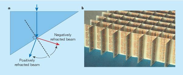

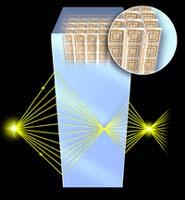
72 Negative refraction
73 Realization of negative refractive index In order to obtain ɛ c (ω)/ɛ 0 = 1 and µ c (ω)/µ 0 = 1, artificial materials are necessary. Common strategy: Periodic structure with inclusions small compared to wavelength. To obtain negative properties, the inclusions are usually resonant. Drawbacks: The inclusions are not always small, putting the material point of view in doubt. The interesting applications require very small losses. The negative properties require frequency variation, making it difficult to maintain negative properties in a large frequency band.
74 Band limitations If the negative properties are realized with passive, causal materials, they must satisfy Kramers-Kronig s relations (ɛ = lim ω ɛ(ω)) ɛ (ω) ɛ = 1 π P ɛ (ω) = 1 π P ɛ (ω ) ω ω dω ɛ (ω ) ɛ ω ω dω These relations represent restriction on the possible frequency behavior, and can be used to derive bounds on the bandwidth where the material parameters can be negative.
75 Example: two Lorentz models ²(!) 4 ² s Re ² 1 Im! ² m=-1 j²(!)-² mj ² m= j²(!)+1j j²(!)-1.5j j²(!)+1j! An ɛ m between ɛ s and ɛ is easily realized for a large bandwidth, whereas an ɛ m < ɛ is not. With fractional bandwidth B: { 1/2 lossy case max ɛ(ω) ɛ m ω B B 1 + B/2 (ɛ ɛ m ) 1 lossless case
76 Outline 1 Plane waves in lossless media General time dependence Time harmonic waves 2 Polarization 3 Propagation in lossy media 4 Oblique propagation and complex waves 5 Paraxial approximation: beams 6 Doppler effect and negative index media 7 Conclusions
77 Conclusions Plane waves are characterized by wave vector k and wave impedance η. Polarization is deduced from time domain electric field. Lossy media leads to complex material parameters, but plane wave formalism remains the same. At oblique propagation, the transverse fields are most important. The paraxial approximation can be used to describe beams. The beam angle depends on the original beam width in terms of wavelengths. The Doppler effect can be used to detect motion. Negative refractive index is possible, but only for very narrow frequency band.
Electromagnetic Wave Propagation Lecture 3: Plane waves in isotropic and bianisotropic media
 Electromagnetic Wave Propagation Lecture 3: Plane waves in isotropic and bianisotropic media Daniel Sjöberg Department of Electrical and Information Technology September 2016 Outline 1 Plane waves in lossless
Electromagnetic Wave Propagation Lecture 8: Propagation in birefringent media
 Electromagnetic Wave Propagation Lecture 8: Propagation in birefringent media Daniel Sjöberg Department of Electrical and Information Technology September 27, 2012 Outline 1 Introduction 2 Maxwell s equations
Electromagnetic Wave Propagation Lecture 5: Propagation in birefringent media
 Electromagnetic Wave Propagation Lecture 5: Propagation in birefringent media Daniel Sjöberg Department of Electrical and Information Technology April 15, 2010 Outline 1 Introduction 2 Wave propagation
Waves. Daniel S. Weile. ELEG 648 Waves. Department of Electrical and Computer Engineering University of Delaware. Plane Waves Reflection of Waves
 Waves Daniel S. Weile Department of Electrical and Computer Engineering University of Delaware ELEG 648 Waves Outline Outline Introduction Let s start by introducing simple solutions to Maxwell s equations
Uniform Plane Waves Page 1. Uniform Plane Waves. 1 The Helmholtz Wave Equation
 Uniform Plane Waves Page 1 Uniform Plane Waves 1 The Helmholtz Wave Equation Let s rewrite Maxwell s equations in terms of E and H exclusively. Let s assume the medium is lossless (σ = 0). Let s also assume
22 Phasor form of Maxwell s equations and damped waves in conducting media
 22 Phasor form of Maxwell s equations and damped waves in conducting media When the fields and the sources in Maxwell s equations are all monochromatic functions of time expressed in terms of their phasors,
Simple medium: D = ɛe Dispersive medium: D = ɛ(ω)e Anisotropic medium: Permittivity as a tensor
e Anisotropic medium: Permittivity as a tensor") Plane Waves 1 Review dielectrics 2 Plane waves in the time domain 3 Plane waves in the frequency domain 4 Plane waves in lossy and dispersive media 5 Phase and group velocity 6 Wave polarization Levis,
Plane Waves 1 Review dielectrics 2 Plane waves in the time domain 3 Plane waves in the frequency domain 4 Plane waves in lossy and dispersive media 5 Phase and group velocity 6 Wave polarization Levis,
EITN90 Radar and Remote Sensing Lecture 5: Target Reflectivity
 EITN90 Radar and Remote Sensing Lecture 5: Target Reflectivity Daniel Sjöberg Department of Electrical and Information Technology Spring 2018 Outline 1 Basic reflection physics 2 Radar cross section definition
Uniform Plane Waves. 2.1 Uniform Plane Waves in Lossless Media. ɛ = 1 ηc, μ = η c, where c = 1 μ. , η = z = 1 c η H. z = 1 E. z = ˆx E y. c t.
 .. Uniform Plane Waves in Lossless Media 37. Uniform Plane Waves in Lossless Media Uniform Plane Waves The simplest electromagnetic waves are uniform plane waves propagating along some fixed direction,
EECS 117. Lecture 22: Poynting s Theorem and Normal Incidence. Prof. Niknejad. University of California, Berkeley
 University of California, Berkeley EECS 117 Lecture 22 p. 1/2 EECS 117 Lecture 22: Poynting s Theorem and Normal Incidence Prof. Niknejad University of California, Berkeley University of California, Berkeley
remain essentially unchanged for the case of time-varying fields, the remaining two
 Unit 2 Maxwell s Equations Time-Varying Form While the Gauss law forms for the static electric and steady magnetic field equations remain essentially unchanged for the case of time-varying fields, the
3.1 The Helmoltz Equation and its Solution. In this unit, we shall seek the physical significance of the Maxwell equations, summarized
 Unit 3 TheUniformPlaneWaveand Related Topics 3.1 The Helmoltz Equation and its Solution In this unit, we shall seek the physical significance of the Maxwell equations, summarized at the end of Unit 2,
Electromagnetic Wave Propagation Lecture 13: Oblique incidence II
 Electromagnetic Wave Propagation Lecture 13: Oblique incidence II Daniel Sjöberg Department of Electrical and Information Technology October 15, 2013 Outline 1 Surface plasmons 2 Snel s law in negative-index
Propagation of Plane Waves
 Chapter 6 Propagation of Plane Waves 6 Plane Wave in a Source-Free Homogeneous Medium 62 Plane Wave in a Lossy Medium 63 Interference of Two Plane Waves 64 Reflection and Transmission at a Planar Interface
Electromagnetic Wave Propagation Lecture 2: Time harmonic dependence, constitutive relations
 Electromagnetic Wave Propagation Lecture 2: Time harmonic dependence, constitutive relations Daniel Sjöberg Department of Electrical and Information Technology September 2, 2010 Outline 1 Harmonic time
Electromagnetic Wave Propagation Lecture 13: Oblique incidence II
 Electromagnetic Wave Propagation Lecture 13: Oblique incidence II Daniel Sjöberg Department of Electrical and Information Technology October 2016 Outline 1 Surface plasmons 2 Snel s law in negative-index
ECE357H1S ELECTROMAGNETIC FIELDS TERM TEST March 2016, 18:00 19:00. Examiner: Prof. Sean V. Hum
 UNIVERSITY OF TORONTO FACULTY OF APPLIED SCIENCE AND ENGINEERING The Edward S. Rogers Sr. Department of Electrical and Computer Engineering ECE357H1S ELECTROMAGNETIC FIELDS TERM TEST 2 21 March 2016, 18:00
EECS 117 Lecture 20: Plane Waves
 University of California, Berkeley EECS 117 Lecture 20 p. 1/2 EECS 117 Lecture 20: Plane Waves Prof. Niknejad University of California, Berkeley University of California, Berkeley EECS 117 Lecture 20 p.
Electromagnetic Waves Across Interfaces
 Lecture 1: Foundations of Optics Outline 1 Electromagnetic Waves 2 Material Properties 3 Electromagnetic Waves Across Interfaces 4 Fresnel Equations 5 Brewster Angle 6 Total Internal Reflection Christoph
Plane Waves Part II. 1. For an electromagnetic wave incident from one medium to a second medium, total reflection takes place when
 Plane Waves Part II. For an electromagnetic wave incident from one medium to a second medium, total reflection takes place when (a) The angle of incidence is equal to the Brewster angle with E field perpendicular
Summary of Beam Optics
 Summary of Beam Optics Gaussian beams, waves with limited spatial extension perpendicular to propagation direction, Gaussian beam is solution of paraxial Helmholtz equation, Gaussian beam has parabolic
Projects in ETEN05 Electromagnetic wave propagation Fall 2012
 Projects in ETEN05 Electromagnetic wave propagation Fall 2012 i General notes Choose one of the projects on the following pages. All projects contain some numerical part, but some more than others. The
10 (4π 10 7 ) 2σ 2( = (1 + j)(.0104) = = j.0001 η c + η j.0104
 2σ 2( = (1 + j)(.0104) = = j.0001 η c + η j.0104") CHAPTER 1 1.1. A uniform plane wave in air, E + x1 E+ x10 cos(1010 t βz)v/m, is normally-incident on a copper surface at z 0. What percentage of the incident power density is transmitted into the copper?
CHAPTER 1 1.1. A uniform plane wave in air, E + x1 E+ x10 cos(1010 t βz)v/m, is normally-incident on a copper surface at z 0. What percentage of the incident power density is transmitted into the copper?
Cartesian Coordinates
 Cartesian Coordinates Daniel S. Weile Department of Electrical and Computer Engineering University of Delaware ELEG 648 Cartesian Coordinates Outline Outline Separation of Variables Away from sources,
5 Electromagnetic Waves
 5 Electromagnetic Waves 5.1 General Form for Electromagnetic Waves. In free space, Maxwell s equations are: E ρ ɛ 0 (5.1.1) E + B 0 (5.1.) B 0 (5.1.3) B µ 0 ɛ 0 E µ 0 J (5.1.4) In section 4.3 we derived
Electromagnetic Wave Propagation Lecture 2: Time harmonic dependence, constitutive relations
 Electromagnetic Wave Propagation Lecture 2: Time harmonic dependence, constitutive relations Daniel Sjöberg Department of Electrical and Information Technology September 2015 Outline 1 Harmonic time dependence
Electrodynamics I Final Exam - Part A - Closed Book KSU 2005/12/12 Electro Dynamic
 Electrodynamics I Final Exam - Part A - Closed Book KSU 2005/12/12 Name Electro Dynamic Instructions: Use SI units. Short answers! No derivations here, just state your responses clearly. 1. (2) Write an
Guided Waves. Daniel S. Weile. Department of Electrical and Computer Engineering University of Delaware. ELEG 648 Guided Waves
 Guided Waves Daniel S. Weile Department of Electrical and Computer Engineering University of Delaware ELEG 648 Guided Waves Outline Outline The Circuit Model of Transmission Lines R + jωl I(z + z) I(z)
Plane Waves GATE Problems (Part I)
") Plane Waves GATE Problems (Part I). A plane electromagnetic wave traveling along the + z direction, has its electric field given by E x = cos(ωt) and E y = cos(ω + 90 0 ) the wave is (a) linearly polarized
Plane Waves GATE Problems (Part I). A plane electromagnetic wave traveling along the + z direction, has its electric field given by E x = cos(ωt) and E y = cos(ω + 90 0 ) the wave is (a) linearly polarized
Multilayer Reflectivity
 Multilayer Reflectivity John E. Davis jed@jedsoft.org January 5, 2014 1 Introduction The purpose of this document is to present an ab initio derivation of the reflectivity for a plane electromagnetic wave
Radio Propagation Channels Exercise 2 with solutions. Polarization / Wave Vector
 /8 Polarization / Wave Vector Assume the following three magnetic fields of homogeneous, plane waves H (t) H A cos (ωt kz) e x H A sin (ωt kz) e y () H 2 (t) H A cos (ωt kz) e x + H A sin (ωt kz) e y (2)
EECS 117. Lecture 23: Oblique Incidence and Reflection. Prof. Niknejad. University of California, Berkeley
 University of California, Berkeley EECS 117 Lecture 23 p. 1/2 EECS 117 Lecture 23: Oblique Incidence and Reflection Prof. Niknejad University of California, Berkeley University of California, Berkeley
Waves in Linear Optical Media
 1/53 Waves in Linear Optical Media Sergey A. Ponomarenko Dalhousie University c 2009 S. A. Ponomarenko Outline Plane waves in free space. Polarization. Plane waves in linear lossy media. Dispersion relations
Physics 506 Winter 2004
 Physics 506 Winter 004 G. Raithel January 6, 004 Disclaimer: The purpose of these notes is to provide you with a general list of topics that were covered in class. The notes are not a substitute for reading
Characterization of Left-Handed Materials
 Characterization of Left-Handed Materials Massachusetts Institute of Technology 6.635 lecture notes 1 Introduction 1. How are they realized? 2. Why the denomination Left-Handed? 3. What are their properties?
Electromagnetic Waves
 Electromagnetic Waves Maxwell s equations predict the propagation of electromagnetic energy away from time-varying sources (current and charge) in the form of waves. Consider a linear, homogeneous, isotropic
26 Standing waves, radiation pressure
 26 Standing waves, radiation pressure We continue in this lecture with our studies of wave reflection and transmission at a plane boundary between two homogeneous media. In case of total reflection from
Typical anisotropies introduced by geometry (not everything is spherically symmetric) temperature gradients magnetic fields electrical fields
 temperature gradients magnetic fields electrical fields") Lecture 6: Polarimetry 1 Outline 1 Polarized Light in the Universe 2 Fundamentals of Polarized Light 3 Descriptions of Polarized Light Polarized Light in the Universe Polarization indicates anisotropy
Lecture 6: Polarimetry 1 Outline 1 Polarized Light in the Universe 2 Fundamentals of Polarized Light 3 Descriptions of Polarized Light Polarized Light in the Universe Polarization indicates anisotropy
1 Chapter 8 Maxwell s Equations
 Electromagnetic Waves ECEN 3410 Prof. Wagner Final Review Questions 1 Chapter 8 Maxwell s Equations 1. Describe the integral form of charge conservation within a volume V through a surface S, and give
PHYS 408, Optics. Problem Set 1 - Spring Posted: Fri, January 8, 2015 Due: Thu, January 21, 2015.
 PHYS 408, Optics Problem Set 1 - Spring 2016 Posted: Fri, January 8, 2015 Due: Thu, January 21, 2015. 1. An electric field in vacuum has the wave equation, Let us consider the solution, 2 E 1 c 2 2 E =
PHYS 110B - HW #5 Fall 2005, Solutions by David Pace Equations referenced equations are from Griffiths Problem statements are paraphrased
 PHYS 0B - HW #5 Fall 005, Solutions by David Pace Equations referenced equations are from Griffiths Problem statements are paraphrased [.] Imagine a prism made of lucite (n.5) whose cross-section is a
ECE357H1F ELECTROMAGNETIC FIELDS FINAL EXAM. 28 April Examiner: Prof. Sean V. Hum. Duration: hours
 UNIVERSITY OF TORONTO FACULTY OF APPLIED SCIENCE AND ENGINEERING The Edward S. Rogers Sr. Department of Electrical and Computer Engineering ECE357H1F ELECTROMAGNETIC FIELDS FINAL EXAM 28 April 15 Examiner:
Essentials of Electromagnetic Field Theory. Maxwell s equations serve as a fundamental tool in photonics
 Essentials of Electromagnetic Field Theory Maxwell s equations serve as a fundamental tool in photonics Updated: 19:3 1 Light is both an Electromagnetic Wave and a Particle Electromagnetic waves are described
Basics of Wave Propagation
 Basics of Wave Propagation S. R. Zinka zinka@hyderabad.bits-pilani.ac.in Department of Electrical & Electronics Engineering BITS Pilani, Hyderbad Campus May 7, 2015 Outline 1 Time Harmonic Fields 2 Helmholtz
9 The conservation theorems: Lecture 23
 9 The conservation theorems: Lecture 23 9.1 Energy Conservation (a) For energy to be conserved we expect that the total energy density (energy per volume ) u tot to obey a conservation law t u tot + i
Dielectric Slab Waveguide
 Chapter Dielectric Slab Waveguide We will start off examining the waveguide properties of a slab of dielectric shown in Fig... d n n x z n Figure.: Cross-sectional view of a slab waveguide. { n, x < d/
Electromagnetic fields and waves
 Electromagnetic fields and waves Maxwell s rainbow Outline Maxwell s equations Plane waves Pulses and group velocity Polarization of light Transmission and reflection at an interface Macroscopic Maxwell
Chapter 3 Uniform Plane Waves Dr. Stuart Long
 3-1 Chapter 3 Uniform Plane Waves Dr. Stuart Long 3- What is a wave? Mechanism by which a disturbance is propagated from one place to another water, heat, sound, gravity, and EM (radio, light, microwaves,
Reflection/Refraction
 Reflection/Refraction Page Reflection/Refraction Boundary Conditions Interfaces between different media imposed special boundary conditions on Maxwell s equations. It is important to understand what restrictions
(12a x +14a y )= 8.5a x 9.9a y A/m
= 8.5a x 9.9a y A/m") Chapter 11 Odd-Numbered 11.1. Show that E xs Ae jk 0z+φ is a solution to the vector Helmholtz equation, Sec. 11.1, Eq. (16), for k 0 ω µ 0 ɛ 0 and any φ and A:We take d dz Aejk 0z+φ (jk 0 ) Ae jk 0z+φ
Chapter 11 Odd-Numbered 11.1. Show that E xs Ae jk 0z+φ is a solution to the vector Helmholtz equation, Sec. 11.1, Eq. (16), for k 0 ω µ 0 ɛ 0 and any φ and A:We take d dz Aejk 0z+φ (jk 0 ) Ae jk 0z+φ
Wavepackets. Outline. - Review: Reflection & Refraction - Superposition of Plane Waves - Wavepackets - ΔΔk Δx Relations
 Wavepackets Outline - Review: Reflection & Refraction - Superposition of Plane Waves - Wavepackets - ΔΔk Δx Relations 1 Sample Midterm (one of these would be Student X s Problem) Q1: Midterm 1 re-mix (Ex:
Fiber Optics. Equivalently θ < θ max = cos 1 (n 0 /n 1 ). This is geometrical optics. Needs λ a. Two kinds of fibers:
. This is geometrical optics. Needs λ a. Two kinds of fibers:") Waves can be guided not only by conductors, but by dielectrics. Fiber optics cable of silica has nr varying with radius. Simplest: core radius a with n = n 1, surrounded radius b with n = n 0 < n 1. Total
Waves can be guided not only by conductors, but by dielectrics. Fiber optics cable of silica has nr varying with radius. Simplest: core radius a with n = n 1, surrounded radius b with n = n 0 < n 1. Total
CHAPTER 9 ELECTROMAGNETIC WAVES
 CHAPTER 9 ELECTROMAGNETIC WAVES Outlines 1. Waves in one dimension 2. Electromagnetic Waves in Vacuum 3. Electromagnetic waves in Matter 4. Absorption and Dispersion 5. Guided Waves 2 Skip 9.1.1 and 9.1.2
ELE3310: Basic ElectroMagnetic Theory
 A summary for the final examination EE Department The Chinese University of Hong Kong November 2008 Outline Mathematics 1 Mathematics Vectors and products Differential operators Integrals 2 Integral expressions
Electrical and optical properties of materials
 Electrical and optical properties of materials John JL Morton Part 4: Mawell s Equations We have already used Mawell s equations for electromagnetism, and in many ways they are simply a reformulation (or
Electromagnetic Theory (Hecht Ch. 3)
") Phys 531 Lecture 2 30 August 2005 Electromagnetic Theory (Hecht Ch. 3) Last time, talked about waves in general wave equation: 2 ψ(r, t) = 1 v 2 2 ψ t 2 ψ = amplitude of disturbance of medium For light,
Phys 531 Lecture 2 30 August 2005 Electromagnetic Theory (Hecht Ch. 3) Last time, talked about waves in general wave equation: 2 ψ(r, t) = 1 v 2 2 ψ t 2 ψ = amplitude of disturbance of medium For light,
Electromagnetic (EM) Waves
 Waves") Electromagnetic (EM) Waves Short review on calculus vector Outline A. Various formulations of the Maxwell equation: 1. In a vacuum 2. In a vacuum without source charge 3. In a medium 4. In a dielectric
Electromagnetic (EM) Waves Short review on calculus vector Outline A. Various formulations of the Maxwell equation: 1. In a vacuum 2. In a vacuum without source charge 3. In a medium 4. In a dielectric
EECS 117. Lecture 25: Field Theory of T-Lines and Waveguides. Prof. Niknejad. University of California, Berkeley
 EECS 117 Lecture 25: Field Theory of T-Lines and Waveguides Prof. Niknejad University of California, Berkeley University of California, Berkeley EECS 117 Lecture 25 p. 1/2 Waveguides and Transmission Lines
Transmission Lines, Waveguides, and Resonators
 Chapter 7 Transmission Lines, Waveguides, and Resonators 1 7.1. General Properties of Guided Waves 7.. TM, TE, and TEM Modes 7.3. Coaxial Lines 7.4. Two-Wire Lines 7.5. Parallel-Plate Waveguides 7.6. Rectangular
Electromagnetic Waves & Polarization
 Course Instructor Dr. Raymond C. Rumpf Office: A 337 Phone: (915) 747 6958 E Mail: rcrumpf@utep.edu EE 4347 Applied Electromagnetics Topic 3a Electromagnetic Waves & Polarization Electromagnetic These
Guided waves - Lecture 11
 Guided waves - Lecture 11 1 Wave equations in a rectangular wave guide Suppose EM waves are contained within the cavity of a long conducting pipe. To simplify the geometry, consider a pipe of rectangular
PLANE WAVE PROPAGATION AND REFLECTION. David R. Jackson Department of Electrical and Computer Engineering University of Houston Houston, TX
 PLANE WAVE PROPAGATION AND REFLECTION David R. Jackson Department of Electrical and Computer Engineering University of Houston Houston, TX 7704-4793 Abstract The basic properties of plane waves propagating
EECS 117 Lecture 26: TE and TM Waves
 EECS 117 Lecture 26: TE and TM Waves Prof. Niknejad University of California, Berkeley University of California, Berkeley EECS 117 Lecture 26 p. 1/2 TE Waves TE means that e z = 0 but h z 0. If k c 0,
Problem 8.18 For some types of glass, the index of refraction varies with wavelength. A prism made of a material with
 Problem 8.18 For some types of glass, the index of refraction varies with wavelength. A prism made of a material with n = 1.71 4 30 λ 0 (λ 0 in µm), where λ 0 is the wavelength in vacuum, was used to disperse
Problem set 3. Electromagnetic waves
 Second Year Electromagnetism Michaelmas Term 2017 Caroline Terquem Problem set 3 Electromagnetic waves Problem 1: Poynting vector and resistance heating This problem is not about waves but is useful to
Theory and Applications of Dielectric Materials Introduction
 SERG Summer Seminar Series #11 Theory and Applications of Dielectric Materials Introduction Tzuyang Yu Associate Professor, Ph.D. Structural Engineering Research Group (SERG) Department of Civil and Environmental
Wave Phenomena Physics 15c. Lecture 15 Reflection and Refraction
 Wave Phenomena Physics 15c Lecture 15 Reflection and Refraction What We (OK, Brian) Did Last Time Discussed EM waves in vacuum and in matter Maxwell s equations Wave equation Plane waves E t = c E B t
Propagation of EM Waves in material media
 Propagation of EM Waves in material media S.M.Lea 09 Wave propagation As usual, we start with Maxwell s equations with no free charges: D =0 B =0 E = B t H = D t + j If we now assume that each field has
Wave Propagation in Uniaxial Media. Reflection and Transmission at Interfaces
 Lecture 5: Crystal Optics Outline 1 Homogeneous, Anisotropic Media 2 Crystals 3 Plane Waves in Anisotropic Media 4 Wave Propagation in Uniaxial Media 5 Reflection and Transmission at Interfaces Christoph
Electromagnetic Theory for Microwaves and Optoelectronics
 Keqian Zhang Dejie Li Electromagnetic Theory for Microwaves and Optoelectronics Second Edition With 280 Figures and 13 Tables 4u Springer Basic Electromagnetic Theory 1 1.1 Maxwell's Equations 1 1.1.1
Electromagnetism. Christopher R Prior. ASTeC Intense Beams Group Rutherford Appleton Laboratory
 lectromagnetism Christopher R Prior Fellow and Tutor in Mathematics Trinity College, Oxford ASTeC Intense Beams Group Rutherford Appleton Laboratory Contents Review of Maxwell s equations and Lorentz Force
Wave Phenomena Physics 15c
 Wave Phenomena Physics 15c Lecture 15 lectromagnetic Waves (H&L Sections 9.5 7) What We Did Last Time! Studied spherical waves! Wave equation of isotropic waves! Solution e! Intensity decreases with! Doppler
ELECTROMAGNETISM SUMMARY
 Review of E and B ELECTROMAGNETISM SUMMARY (Rees Chapters 2 and 3) The electric field E is a vector function. E q o q If we place a second test charged q o in the electric field of the charge q, the two
So far, we have considered three basic classes of antennas electrically small, resonant
 Unit 5 Aperture Antennas So far, we have considered three basic classes of antennas electrically small, resonant (narrowband) and broadband (the travelling wave antenna). There are amny other types of
EM waves: energy, resonators. Scalar wave equation Maxwell equations to the EM wave equation A simple linear resonator Energy in EM waves 3D waves
 EM waves: energy, resonators Scalar wave equation Maxwell equations to the EM wave equation A simple linear resonator Energy in EM waves 3D waves Simple scalar wave equation 2 nd order PDE 2 z 2 ψ (z,t)
Electromagnetic Waves For fast-varying phenomena, the displacement current cannot be neglected, and the full set of Maxwell s equations must be used
 Electromagnetic Waves For fast-varying phenomena, the displacement current cannot be neglected, and the full set of Maxwell s equations must be used B( t) E = dt D t H = J+ t D =ρ B = 0 D=εE B=µ H () F
3 Constitutive Relations: Macroscopic Properties of Matter
 EECS 53 Lecture 3 c Kamal Sarabandi Fall 21 All rights reserved 3 Constitutive Relations: Macroscopic Properties of Matter As shown previously, out of the four Maxwell s equations only the Faraday s and
Goal: The theory behind the electromagnetic radiation in remote sensing. 2.1 Maxwell Equations and Electromagnetic Waves
 Chapter 2 Electromagnetic Radiation Goal: The theory behind the electromagnetic radiation in remote sensing. 2.1 Maxwell Equations and Electromagnetic Waves Electromagnetic waves do not need a medium to
A Review of Basic Electromagnetic Theories
 A Review of Basic Electromagnetic Theories Important Laws in Electromagnetics Coulomb s Law (1785) Gauss s Law (1839) Ampere s Law (1827) Ohm s Law (1827) Kirchhoff s Law (1845) Biot-Savart Law (1820)
Antennas and Propagation
 Antennas and Propagation Ranga Rodrigo University of Moratuwa October 20, 2008 Compiled based on Lectures of Prof. (Mrs.) Indra Dayawansa. Ranga Rodrigo (University of Moratuwa) Antennas and Propagation
Transmission Line Theory
 S. R. Zinka zinka@vit.ac.in School of Electronics Engineering Vellore Institute of Technology April 26, 2013 Outline 1 Free Space as a TX Line 2 TX Line Connected to a Load 3 Some Special Cases 4 Smith
Lecture 5 Notes, Electromagnetic Theory II Dr. Christopher S. Baird, faculty.uml.edu/cbaird University of Massachusetts Lowell
 Lecture 5 Notes, Electromagnetic Theory II Dr. Christopher S. Baird, faculty.uml.edu/cbaird University of Massachusetts Lowell 1. Waveguides Continued - In the previous lecture we made the assumption that
Lecture 2 Notes, Electromagnetic Theory II Dr. Christopher S. Baird, faculty.uml.edu/cbaird University of Massachusetts Lowell
 Lecture Notes, Electromagnetic Theory II Dr. Christopher S. Baird, faculty.uml.edu/cbaird University of Massachusetts Lowell 1. Dispersion Introduction - An electromagnetic wave with an arbitrary wave-shape
UNIT I ELECTROSTATIC FIELDS
 UNIT I ELECTROSTATIC FIELDS 1) Define electric potential and potential difference. 2) Name few applications of gauss law in electrostatics. 3) State point form of Ohm s Law. 4) State Divergence Theorem.
Electromagnetic Theorems
 Electromagnetic Theorems Daniel S. Weile Department of Electrical and Computer Engineering University of Delaware ELEG 648 Electromagnetic Theorems Outline Outline Duality The Main Idea Electric Sources
Jackson 7.6 Homework Problem Solution Dr. Christopher S. Baird University of Massachusetts Lowell
 Jackson 7.6 Homework Problem Solution Dr. Christopher S. Baird University of Massachusetts Lowell PROBLEM: A plane wave of frequency ω is incident normally from vacuum on a semi-infinite slab of material
Electromagnetic Wave Propagation Lecture 1: Maxwell s equations
 Electromagnetic Wave Propagation Lecture 1: Maxwell s equations Daniel Sjöberg Department of Electrical and Information Technology September 3, 2013 Outline 1 Maxwell s equations 2 Vector analysis 3 Boundary
1 Electromagnetic concepts useful for radar applications
 Electromagnetic concepts useful for radar applications The scattering of electromagnetic waves by precipitation particles and their propagation through precipitation media are of fundamental importance
Physics 3323, Fall 2014 Problem Set 13 due Friday, Dec 5, 2014
 Physics 333, Fall 014 Problem Set 13 due Friday, Dec 5, 014 Reading: Finish Griffiths Ch. 9, and 10..1, 10.3, and 11.1.1-1. Reflecting on polarizations Griffiths 9.15 (3rd ed.: 9.14). In writing (9.76)
Chap. 1 Fundamental Concepts
 NE 2 Chap. 1 Fundamental Concepts Important Laws in Electromagnetics Coulomb s Law (1785) Gauss s Law (1839) Ampere s Law (1827) Ohm s Law (1827) Kirchhoff s Law (1845) Biot-Savart Law (1820) Faradays
Lecture 21 Reminder/Introduction to Wave Optics
 Lecture 1 Reminder/Introduction to Wave Optics Program: 1. Maxwell s Equations.. Magnetic induction and electric displacement. 3. Origins of the electric permittivity and magnetic permeability. 4. Wave
H ( E) E ( H) = H B t
 E ( H) = H B t") Chapter 5 Energy and Momentum The equations established so far describe the behavior of electric and magnetic fields. They are a direct consequence of Maxwell s equations and the properties of matter.
Chapter 5 Energy and Momentum The equations established so far describe the behavior of electric and magnetic fields. They are a direct consequence of Maxwell s equations and the properties of matter.
GUIDED MICROWAVES AND OPTICAL WAVES
 Chapter 1 GUIDED MICROWAVES AND OPTICAL WAVES 1.1 Introduction In communication engineering, the carrier frequency has been steadily increasing for the obvious reason that a carrier wave with a higher
GENERALIZED SURFACE PLASMON RESONANCE SENSORS USING METAMATERIALS AND NEGATIVE INDEX MATERIALS
 Progress In Electromagnetics Research, PIER 5, 39 5, 005 GENERALIZED SURFACE PLASMON RESONANCE SENSORS USING METAMATERIALS AND NEGATIVE INDEX MATERIALS A. Ishimaru, S. Jaruwatanadilok, and Y. Kuga Box
1 The formation and analysis of optical waveguides
 1 The formation and analysis of optical waveguides 1.1 Introduction to optical waveguides Optical waveguides are made from material structures that have a core region which has a higher index of refraction
Spherical Waves. Daniel S. Weile. Department of Electrical and Computer Engineering University of Delaware. ELEG 648 Spherical Coordinates
 Spherical Waves Daniel S. Weile Department of Electrical and Computer Engineering University of Delaware ELEG 648 Spherical Coordinates Outline Wave Functions 1 Wave Functions Outline Wave Functions 1
Fourier Approach to Wave Propagation
 Phys 531 Lecture 15 13 October 005 Fourier Approach to Wave Propagation Last time, reviewed Fourier transform Write any function of space/time = sum of harmonic functions e i(k r ωt) Actual waves: harmonic
D. S. Weile Radiation
 Radiation Daniel S. Weile Department of Electrical and Computer Engineering University of Delaware ELEG 648 Radiation Outline Outline Maxwell Redux Maxwell s Equation s are: 1 E = jωb = jωµh 2 H = J +
Waveguides and Cavities
 Waveguides and Cavities John William Strutt also known as Lord Rayleigh (1842-1919) September 17, 2001 Contents 1 Reflection and Transmission at a Conducting Wall 2 1.1 Boundary Conditions...........................
For the magnetic field B called magnetic induction (unfortunately) M called magnetization is the induced field H called magnetic field H =
 M called magnetization is the induced field H called magnetic field H =") To review, in our original presentation of Maxwell s equations, ρ all J all represented all charges, both free bound. Upon separating them, free from bound, we have (dropping quadripole terms): For the
To review, in our original presentation of Maxwell s equations, ρ all J all represented all charges, both free bound. Upon separating them, free from bound, we have (dropping quadripole terms): For the