AN ENGINEERING MODEL FOR SOLAR ENERGETIC PARTICLES IN INTERPLANETARY SPACE

Transcription

1 AN ENGINEERING MODEL FOR SOLAR ENERGETIC PARTICLES IN INTERPLANETARY SPACE Angels Aran 1,3, Blai Sanahuja 1,3,4 and David Lario 2 (1) Departament d Astronomia i Meteorologia. Universitat de Barcelona Martí i Franquès Barcelona (Spain) Phone.: ; fax: aaran@am.ub.es, Blai.Sanahuja@ub.edu (2) The Johns Hopkins University. Applied Physics Laboratory Johns Hopkins Rd. Laurel, MD United States Phone: ; David.Lario@jhuapl.edu (3) Institut d Estudis Espacials de Catalunya (IEEC) Gran Capità Barcelona (Spain) (4) CER d Astrofísica, Física de Partícules i Cosmologia. Unitat Associada a l Institut de Ciències de l Espai del CSIC Universitat de Barcelona. Martí i Franquès Barcelona (Spain) FINAL REPORT (Contract 14098/99/NL/MM, extended) ESA/ESTEC, December 2003 (Revised, April 2004)

2

3 Table of Contents Introduction 9 1 Solar energetic particle events Origin and characteristics Large gradual SEP events Models of gradual SEP events Radial dependence of particle fluxes 32 2 Our modeling of SEP events Summary of the overall scheme The shock-particle model The particle transport equation The MHD simulation of interplanetary shock Deriving the injection rate and its energy dependence Weak points of the scenario and the model Our scenario and model Comparison with other published models Initial conditions of the code The logq - VR relation and the proton flux at high energy The proton flux in the downstream region 55 3 The operational code SOLPENCO Introduction The data base Basic variables 59

4 Comments on the basic values Sources of accelerated particles Injection rate of shock-accelerated particles Injection of solar-accelerated particles Influence of the k-values in synthetic the flux profiles The initial user interface Performing the procedure Reading the data base Internal structure of the data base The interpolation procedure Checking the algorithm of interpolation Computing the fluence Outputs of the code 73 4 Dependence on the energy. The fluence The spectral index γ Dependence of the injection rate Q Discussion of the outputs. Ros03 comments Energy and mean free path Turbulent foreshock region Initial shock velocity Peak flux The fluence Dependence on the shock initial velocity and the heliolongitude Magnitude of the total fluence Fluences at 1.0 AU and at 0.4 AU 110

5 5 5 Modeling SEP events for space weather purposes Introduction The 4-6 April 2000 SEP event Simulation of the shock propagation Simulation of the SEP event Evolution and spectrum of the injection rate Q Dependence of Q on VR and BR The 15 September 2000 and 2 October 1998 SEP events Short description of observations and modeling The spectral index and the Q(VR) relation derived Comparing SOLPENCO with real SEP events The 4-6 April 2000 event (Apr00) The April 1979 event (Apr79) The February 1979 event (Feb79) Summary References Epilogue 155 Appendix A 157 A.1. Lario et al. (1998) paper. [Lar98] 157 A.2. Figures of proton flux anisotropies 177 A.2.1. From Heras et al. (1994) 177 A.2.2. From Heras et al. (1995) 178 A.3. Example of an ESP flux and anisotropy fit 179

6 6 A.4. Differential flux, intensity and anisotropy. Transformation of units 180 A.5. Example of a web interface 182 Appendix B 185 B.1. Shock values derived at 1.0 AU 185 B.2. Shock values derived at 0.4 AU 188 Appendix C 191 C.1. Influence of the k-values in the flux profiles 191 C.2. Checking the interpolation procedure 193 Appendix D 201 The executive script of SOLPENCO 201 Appendix E 217 Values of Q 0 and k derived from the modeled SEP events 217 Appendix F 221 Modeling SEP events. Potential candidates 221 Appendix G 231 G.1. Apr00 event. Evolution of VR and BR ratios for two MHD shock simulations 231 G.2. Apr00 event. Proton population from different IMF flux tubes 233

7

8

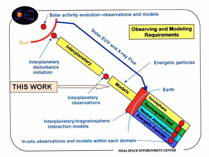
9 INTRODUCTION Solar Energetic Particle (SEP) events in the energy range of 1 MeV to 1 GeV present one of the most severe hazards in the space environment. Such events, highly statistical in nature, tend to occur during periods of intense solar activity, and can lead to high radiation doses in short time intervals. For many deleterious effects the relevant parameter is the total fluence of particles accumulated during a mission, while for others is the maximum particle intensity observed during a single event. Sporadic increases in the energetic particle fluxes can directly affect human endeavors like aerospace technology or the space exploration. The effect of cumulative particle flux might have severe implications for the lifetime of the satellites and the performance of the instruments onboard the spacecraft. Earth s magnetic field can partially shield lowaltitude Earth orbiting satellites, but in the interplanetary medium, or even at high altitude and high latitude Earth orbits, the radiation conditions can be very hostile (Siscoe et al., 2000). SEPs can also play a critical role in understanding the chemistry of Earth s atmosphere (e.g., Jackman and McPeters, 1987). The threat that they pose to manned spaceflights and to spacecraft operations has been reviewed by several authors, see for example, Feynman and Gabriel (2000), and references quoted there. Reames (2001) reviews the space weather hazards due to SEPs in interplanetary space. We refer to Koskinen et al. (2001) for a global description of the space weather effects of SEPs. The most significant sources of energetic particles in the interplanetary medium are both solar flares and interplanetary shocks driven by coronal mass ejections (CMEs). The energetic particle flux enhancements produced by these solar events may last several days and are very hard to predict in advance. The current understanding of the generation, acceleration, and propagation of solar energetic particles in the inner solar system is incomplete because of their random nature and the insufficient knowledge of the physical principles ruling them. In fact, our present ability to forecast solar energetic particle events in space is far from being satisfactory (Turner, 2001). The ANSER report (Turner, 1996) notes hat the lack of a method to observe or account for interplanetary shocks and coronal mass ejections is one of the major deficiencies of quantitative solar proton event predictions (see figure I.1). Heckman et al. (1992) stated Our operational experience suggests the failure to include the effects of interplanetary shocks is a major deficiency with the present version of the model. In some cases the effects were confined to particles with energies near 10 MeV... Beyond shocks, we are unable to asses the source of the order-of-magnitude variation of the observed flux from the predictions. These major events, however, drive the

10 10 design of spacecraft and onboard instrumentation. Therefore, it is important for future missions going closer to Sun or to Mars, to quantify the level of expected radiation. Figure I.1. Flux and cumulative fluence of the October 19-20, 1989, particle event as measured by the GOES spacecraft (from Turner, 2001). Hence, the recommendations of the USA Space Weather Architecture Study Transition Plan (1999; paragraph , Recommendation Robust R&D), that will guide the future investment, development and acquisition of space instrumentation and space-related Space Weather capabilities: (1) Provide a robust Space Weather research and develop a program to implement and improve models, as well as provide options for further growth; (2) Continue to leverage research and development of missions, and enhance operational products until new operational systems are ready. It is important to point out that Space Weather technology still has a meager scientific base, the summary of the report states: Space Weather is a technically immature discipline and basic research leading to physics based models is vital.

11 11 Risk management strategies to study and forecast the effects of energetic particles produced by solar and interplanetary sources are faced with three fundamental approaches: (i) Use of statistical operational algorithms presently in use at forecast centers. (ii) Use of numerical codes for the transport of energetic particles that are currently applied to cosmic ray propagation in an ionized and magnetized environment. And (iii) development of numerical codes for the study of magnetohydrodynamic (MHD) phenomena in the magnetosphere and interplanetary medium. Here we will only address the two last aspects because our concern is with single solar particle events that unexpectedly take place at almost any time during each solar cycle (like in the last week of October 2003 and holding the two following weeks known as the Halloween 2003 events), but certainly more frequently during the most active periods of the solar cycle. Statistical models estimate the cumulative exposure to solar protons over a period of time, in basis of SEP event data from previous solar cycles (i.e. King, 1974; Feynman et al., 1993; and Nymmik, 1998). The standard model of this type is the JPL-91 interplanetary proton fluence model (Feynman et al., 1993 and 2002). Gabriel and Feynman (1996) and Feynman et al. (2002) re-examine various aspects of this model, mainly focusing on the adequacy of the fit of distribution at high energy (1 60 MeV), and Rosenqvist and Hilgers (2003) discuss on its sensitivity with respect the inclusion of new SEP events in the data set used performing predictions. Statistical models are based on statistical approaches and not on single events. It is worthwhile to note that (i) extreme large events, such as August 1972 and October 1989, may dominate the total fluence during a solar cycle, and those events tend to occur under very special conditions of the heliosphere (Kallenrode and Cliver, 2001; Lario and Decker, 2001 and 2002) which are difficult to predict and will not always be present in all solar cycles. And (ii) In certain situations, Statistical forecasting can yield to a false sense of security (Turner, 2001). For example, during the active solar period between 1989 and 1991, there were about 970 days without any SEP event and 120 days with a SEP event in progress. Turner (2001) concludes that if during this period a three-daypersistence criterion is used for forecasting, the forecaster would be right more than 90 % of the time; he would also have, however, a 100 % of security about the prediction prior to each of ~30 SEP events that did occur. Predicting the flux and fluence of large SEP events days or hours in advance is a formidable challenge. The whole process should be as follows. The forecaster must predict (i) where, when and how a CME will occur, (ii) specify the characteristics of the CME, such as location, size, speed, and its ability to drive a shock wave; (iii) determine the efficiency of the shock driven by the CME to accelerate particles to high energies, as well as how the particles will be injected into the interplanetary medium;

12 12 and finally (iv) forecast how these particles and the CME-driven shock will travel through the ambient solar wind. The objective of this project is to develop an engineering code SOLPENCO (standing for SOLar Particle ENgineering COde) for characterizing SEP events at user-specified locations in space from outside the solar corona to the orbit of the Earth. This code estimates time-dependent proton fluxes and fluences as a function of the particle energy over the range of 500 kev to 50 or 100 MeV. It provides a familiar user interface for running the engineering tool that allows the generation of time-intensity profiles for several SEP events. This code does not intend to solve the overall problem, but just provides a first step to the prediction of particle fluxes during SEP events. Our mid-term objectives, beyond the scope of this project, are (i) validate SOLPENCO by performing a statistical comparative analysis of SEP flux and fluence predictions with actual energetic particle observations, and (ii) include estimations for SEP flux and fluences up to the orbit of Mars. The outline of this report is as follows. The first chapter summarizes the main characteristics of the solar energetic particle events that SOLPENCO is aimed to forecast. We also outline the main features of the existing theoretical models in which potential operational codes (like SOLPENCO) relay. It is not our aim to produce an exhaustive review of the state-of-the-art of the field, but only to describe the observational scenario assumed by the theoretical models of SEP events. We quote the main references to provide links to the reader interested in a more thorough lecture or review. The second chapter deals with the specific scenario and model in which our operational code is based. We describe the main features of the code and discuss its weak points, in order to be aware of what will be needed to improve in the future. We will point out that most of these weaknesses are common to all the current existing models of SEP events. We will also shortly comment the intrinsic interest of our model for space weather applications. The third chapter describes the structure of SOLPENCO, its technical characteristics, the data base and the input and output interface. In the fourth chapter we present and discuss various topics related to the code, in particular the recent review by Rosenqvist (2003, hereafter Ros03) of a preliminary version of our code; we comment and discuss the conclusions drawn by Ros03 that are relevant to our work. In chapter five we present the SEP events modeled in order to better understand the variables and parameters used in the code; we outline the main conclusions and their effects in the code. Chapter six lists the references used in this report. A set of appendices contain complementary material. Many people have given us advice or support, thus directly or indirectly contributing to this project. We are grateful to all of them, but we would particularly like to thank Ada Ortiz, Vicente Domingo, Lisa Rosenqvist, Alain. Hilgers, Ana Maria Heras, Eamonn Daly, Murray Dryer, Tom Detman and Zdenka Smith. This work has been supported by

13 13 the ESA/ESTEC Contract 14098/99/NL/NM ( ) and by the project AYA of the Spanish MInisterio de Ciencia y Tecnología. We also acknowledge the computational support provided by the Centre de Supercomputació de Catalunya (CESCA).

14

15 1. SOLAR ENERGETIC PARTICLE EVENTS There are various sources of energetic particles in interplanetary space; the most important are the solar events and the galactic cosmic rays. For the energy range of interest in space weather (basically, protons between 500 kev to ~100 MeV) the flux of SEPs prevails over the other particle populations of diverse origin, i.e. galactic, magnetospheric, or interplanetary in the form of corotating interaction regions (Mewaldt et al., 2002). The interplanetary environment caused by galactic cosmic rays is rather easy to predict. Cosmic rays are always present and the factors that determine their flux over the different phases of the solar cycle are relatively well understood (Mewaldt et al., 1988). We will not discuss them further; see, for example, Smart and Shea (1985) for more information. The prediction of SEP events is more challenging because these particles appear in space sporadically; occasionally three or four times per solar cycle SEP events are very intense. The underlying physical mechanisms involved in the production and development of SEP events are complex and they are not completely understood. The correct understanding of these mechanisms and their proper description by dynamic models are essential to advance and improve the space weather applications ORIGIN AND CHARACTERISTICS SEP events have always been associated with events taking place at the Sun, such as flares, filament disappearances and coronal mass ejections (CMEs). The current working paradigm (under debate, as we will comment later) distinguishes two basic types of SEP events, the impulsive and the gradual events. The origins and current usage of these terms have been reviewed by Cliver and Cane (2002), we refer to that paper for a description of the usefulness and limitations of these terms. Under this paradigm, it is believed that impulsive particle events have their origin during rapid flares while gradual particle events are associated with shocks driven by CMEs. Consistently, SEP intensities are correlated with CME speeds, although it is not uncommon to find SEP intensities over a range of four orders of magnitude for a given CME speed (Kahler et al., 2001).

16 16 Impulsive events are observed in a narrow cone of longitudes corresponding to observers magnetically well-connected to the site of the progenitor solar flare. Conversely, gradual events are observed in a wide-spread range of longitudes regardless of the associated solar flare location, if a flare can be identified at all. Impulsive events are about hundred times more frequent than gradual events at the maximum of the solar cycle. However, impulsive events have typical durations of the order of hours and are less intense than gradual events which can last several days. figure 1.1 shows one example of each type of these events. The detailed characteristics and properties of the two classes of events have been described elsewhere (see Reames 1999, for a review). Figure 1.1. Intensity-time profiles of ions for an impulsive (left) and a gradual (right) SEP event of the year 2000 as measured by ACE/EPAM (Gold et al., 1998). The two lower traces (high energy channels) are proton observations from IMP-8/CPME (Sarris et al., 1976). Large gradual SEP events are associated with fast CMEs (Kahler, 2001). However, fast CMEs tend to occur in association with flares (Harrison, 1995; Nitta and Akiyama, 1999) and hence the difficulty to distinguish what process contributes (and with which percentage) to the development of a SEP event. To rule out the possibility that both processes contribute to a given energetic particle event, it is essential to find pure cases of gradual events not associated with solar flares. Those events are usually associated with filament eruptions (Domingo et al., 1981; Sanahuja et al., 1983 and1991; and Kahler et al., 1986) and in one case with a huge X-ray arcade (Kahler et al., 1998). These events are usually observed at low (less than ~50 MeV) proton

17 17 energies. Cane et al. (2002) suggested that for the most energetic events associated only with disappearing filaments (i.e. Kahler et al., 1986) there are also signatures of flare activity that contributed to the SEP event (see discussion in Cane et al., 2002). In the same way as large gradual SEP events are usually associated with solar events involving both flares and CMEs, it is interesting to note that there are impulsive SEP events, such as the event shown in figure 2, that are associated with narrow CMEs (e.g., Kahler et al., 2001). Reames (2002) proposed that the origin of the two classes of SEP events (i.e. impulsive vs. gradual) lies in the magnetic topology at the Sun at the moment of the solar activity triggering the SEP event. Impulsive events result from resonant stochastic acceleration in magnetic reconnection regions that incorporate open magnetic field lines, allowing both accelerated particles and hot plasma to escape into the interplanetary medium in the form of beam of particles and narrow CMEs or jets, respectively (Kahler et al., 2001). By contrast, in large gradual events, magnetic reconnection occurs on closed field lines beneath closed flux ropes formed in the solar corona. The acceleration and injection of particles able to propagate along open interplanetary magnetic field (IMF) lines only occurs when the flux rope expands through the corona and the interplanetary medium being able to drive a shock wave efficient accelerator of particles from the ambient plasma of the corona and solar wind. Therefore, according to Reames (2002), energetic particles observed in gradual SEP events are accelerated solely by the CME-driven shock, and flares play no role in the production of SEPs. This simple scenario may be disturbed by the wide variety of conditions and processes that may occur during the eruption of a flux rope (Klimchuck, 2001), including dynamic flare processes that may open temporary and locally the field, possible magnetic connectivity of the flare site to open field lines (Aschwanden, 2002), and also some magnetic reconnection processes that involve open field lines, such as the magnetic breakout model proposed by Antiochos et al. (1999). The separation between impulsive SEP events from flares and gradual events from CME-driven shocks has also been challenged by recent composition measurements from the ACE spacecraft. Cohen et al. (1999) showed that at energies >10 MeV/nucleon certain gradual events have compositions and charge states typical of impulsive events. Mewaldt et al. (2002) showed that most solar particles with >5 MeV/nucleon are not simply an accelerated sample of the average solar wind as observed at 1 AU, but a population of particles accelerated within a few solar radii of the Sun. Desai et al. (2001) showed that SEP events associated with interplanetary CME-driven shocks may show 3 He ion enhancements with abundances substantially greater than those measured in the solar wind and typically assumed for gradual events. On the other hand, von Rosenvinge et al. (2001) found a dependence of the heavy ion abundances with respect to the solar longitude of the associated flare event,

18 18 suggesting that, for magnetically well-connected events, flare-associated particles may contribute to the particle intensities observed at Earth. Therefore, the classification of an event as impulsive or gradual does not always clarify the acceleration history of the solar energetic particles (Ruffolo, 2002). Cane et al. (2003) study the Fe/O ratios of twenty nine intense SEP events observed in the energy range MeV/nuc. Their main conclusion is that the observed ratios are consistent with a population of flareaccelerated particles in most of the major SEP events. Therefore, the classification of a SEP event as gradual or impulsive does not distinguish the origin of the particles and the mechanisms that accelerated them. One of the concerns about the two-class paradigm is the ability of the shocks to accelerate coronal and solar wind particles rapidly to GeV energies (Cliver et al., 2002). Most of these relativistic particle events are well associated with flares producing gradual X-ray bursts, long-lasting soft X-ray and centimetric-decametric radio emission. A key issue to determine when energetic particles start being injected is to compare flare emissions with release time of energetic particles. The observed delays between CME launch times and the release times of both near-relativistic electrons (Simnett et al., 2002) and relativistic (> 500 MeV) protons (Kahler, 1994) indicate that the injection of energetic particles begins when CMEs are at a heliocentric radial distance between 2 R and 5 R (see also Kahler et al., 2003). Alternative scenarios to the flare and CME-driven shock particle acceleration suggest that at the time of the CME liftoff, it is possible to produce simultaneously soft X-ray flares as well as coronal shocks which initiate particle acceleration in regions apart from the flare site (Torsti et al., 2001). Particle injection from coronal sites widely separated from the flare site and delayed with respect to the main flare phase and CME launch have been also inferred from radio, optical and extreme ultraviolet observations (Klein and Trottet, 2001, and references therein) suggesting that particle acceleration may occur in the post-phase of solar eruptions. However, Kahler et al. (2000) rebutted this possibility of post-eruptive coronal arcades contributing to gradual SEP events. Cane et al. (2002) also compared SEP events with long-duration, lowfrequency, fast-drift radio bursts, and suggested that type III-l bursts are caused by electron beams of a few tens of kev accelerated during the gradual phase of flares in the reconnection regions associated with the departure of CMEs. In order to clarify the origin of energetic particles and the mechanism that accelerate them, it is essential to study the relationship between flares and CMEs, the timing between the temporary opening of magnetic fields in flaring regions, the occurrence of interplanetary type III bursts, the processes that accelerate particles to high energies, and the coronal altitude where shocks form and particle acceleration occurs.

19 19 There has been a lot of debate on the origins of SEPs (Cliver et al., 2002). There is yet no scientific consensus on the primary source of these particles or on the initial physical mechanisms that accelerate particles to high energies. The US National Space Weather Strategic Plan (1997) evaluated this situation and estimated a period of years before a reliable scientific model is achieved (figure 1.2). By reliable we understand a model in which the scientific community can obtain quantitative and precise forecasting tools for SEPs. At present, it is hard to build a reliable application to predict where, when and how a SEP event will occur. However, based on the observation of previous events, we can model the processes leading to specific timeintensity profiles, energy spectra evolution, fluences and abundances of individual SEP events, especially for gradual events where the acceleration of particles (in particular for low-energy ions) is dominated by acceleration processes in the interplanetary medium by CME-driven shocks. Figure 1.2. Operational models in space weather. A tentative foresight of SEP events and CME propagation forecast (NOAA/SEC 2001, private communication).

20 LARGE GRADUAL SEP EVENTS Large long-lasting SEP events are important mainly for two reasons: their space weather implications (Kahler, 2001), and their dominant contribution to the fluence of energetic particles observed throughout a solar cycle (Shea and Smart, 1996). Large SEP events are well correlated with fast CMEs (Kahler, 2001), although the converse is not true, there are fast CMEs without associated SEP event. The presence of fast CMEs propagating into a slower medium involves the existence of a shock wave. Regardless of the primary processes initiating the acceleration and injection of energetic particles, we will assume that the acceleration and injection of particles throughout the SEP event are dominated by the processes of shock acceleration. Therefore, we will assume the initial perturbation generated as a consequence of the solar eruption is able to drive a shock wave that propagates across the solar corona and through the interplanetary medium. If the conditions are appropriate, this shock accelerates particles from the ambient plasma (or accelerates particles also from contiguous or previous solar events), and injects them at the base of the IMF lines. These energetic particles stream out along these lines en route to Earth and to spacecraft located in the interplanetary medium. Figure 1.3 sketches this scenario; it shows how the shock propagates away from the Sun, expanding in the interplanetary medium and how its front intersects the IMF lines. Once shockaccelerated have been injected in the interplanetary medium, moving upstream (as indicated in the figure) or downstream the shock, they propagate along the IMF lines, towards the observer. Interplanetary shocks accelerate particles more efficiently at low than at high energies (e.g., Forman and Webb, 1985). When the observer is located at 1 AU from the Sun, it is quite usual to see a small peak, if any, on the 1 MeV proton flux at the shock passage, while a jump from one to three orders of magnitude is observed in the flux at ~100 kev. Figure 1.4 shows the proton differential flux for ten energy channels between 115 kev and 96 MeV, observed at 1 AU by the ACE and IMP-8 spacecraft. This SEP event is associated with an interplanetary shock that reached ACE on the 28 of October 2000 (doy 302). At high energies (> 5 MeV), a large fraction of protons was already accelerated when the shock was close to the Sun. At lower energies (< 1 MeV), however, the shock was still an efficient particle-accelerator when it arrived at ACE. Low-energy (< 1 MeV) proton fluxes usually peak around the arrival of the shock (Lario et al., 2003). The particle intensity enhancement associated with the shock passage is known as the Energetic Storm Particle (ESP) event. For certain SEP events (i.e. figure I.1) the shock-enhanced peak accounts for over the sixty per cent of the total fluence measured during the event (Turner, 2001).

21 21 1) 2) 3) 4) Figure 1.3. These four plots sketch how a shock generated by a CME propagates away from the Sun and expands in the interplanetary medium. Its front intersects the IMF and shock-accelerated particles stream away along them (upstream, green arrows). The red point identifies the point of the shock front that magnetically connects to the observer (identified by a green diamond); this point has been named cobpoint by Heras et al. (1995). The red arrow indicates that the cobpoint moves toward the nose of the shock (in this case) as the shock approaches the observer. Therefore, we will assume that shocks accelerate particles since their formation close to the Sun and continue accelerating particles as they move away from the Sun. particles are accelerated at the coronal or interplanetary shocks by a Fermi mechanism for quasi-parallel shocks (Jokipii, 1982; Lee 1982) and gradient-drift acceleration for quasi-perpendicular shocks (Hudson, 1965; Armstrong et al., 1977). As the shock expands in the interplanetary medium, it is assumed to weaken and therefore becoming less and less efficient at accelerating particles to high energies. In order to explain observations of SEP events by multiple spacecraft magnetically

22 22 Figure 1.4. Intensity-time profiles of protons for the SEP event of 29 October 2000, as measured by ACE/EPAM (Gold et al., 1998); the four higher energy channels are proton observations from IMP-8/CPME (Sarris et al., 1976). It is worth to realize the different evolution of these profiles at low and high energy, which reflects the contribution to the flux of shock-accelerated particles. connected to regions of the Sun distant from the parent solar active region, it is assumed that, in some cases, the shocks may extend up to 300 in longitude near the corona (Cliver et al., 1995). However, interplanetary shocks observed at 1 AU extend at most 180 in longitude (Cane, 1988). It is worth to point out that the extension of the front of shock able to efficiently accelerate particles could be smaller than this value, and becoming even smaller as the energy of the particles considered increases. The presence of shock-accelerated particles in large SEP events can be also tracked from the evolution of the first order parallel anisotropy (as defined by Sanderson et al., 1985) of the particle population, either in the upstream part of the SEP event (ahead of the shock) or from the change of its value across the shock. Heras et al. (1994)

23 23 demonstrated that large SEP events can show very high anisotropies (> 0.2) during many hours; between 5 and 36 hours in the upstream region of the shock, depending on the heliolongitude of the solar source which triggers the SEP event. The two first figures of appendix A.2 (see Heras et al., 1994, for more details) illustrate the case; figure A shows three different SEP events that were generated from different solar longitudes and that displayed large and long-lasting anisotropies. Figure A shows the dependence of the anisotropy with respect to the heliolongitude of the parent solar event. Due to its relevant physical meaning, particle flux anisotropy is a standard observational variable that must be taken into consideration and fitted when modeling particle events, a fact that today is frequently forgotten by modelers. Figure A of the same appendix shows a simultaneous fit of ~0.8 MeV proton flux and anisotropy profiles in the upstream region of the shock for three different SEP events, which are similar to those shown in figure A The study of anisotropies also reveals the flow pattern of particles through the front of the shock. In many intense and long-lasting SEP events generated from the western hemisphere of the Sun (known as western SEP events) or from longitudes close to the Sun-Earth field line (known as Central Meridian SEP events), the first-order anisotropy of low-energy (< 2 MeV) protons reverses its sense at the shock arrival (Domingo et al., 1989). For intense SEP events generated from the east hemisphere of the Sun (known as eastern SEP events; i.e. these events where the magnetic connection between the shock and the observer is established only a few hours before the shock arrival) this anisotropy reversing frequently takes several minutes or hours after the shock passage, if it happens at all, and is energy dependent. Sanahuja and Domingo (1987) identified the same pattern analyzing the low-energy proton population as an independent population in the solar wind. This relevant observational fact represents a further constraint for SEP models trying to describe particle fluxes in the downstream region of shocks, but there are no models for this region, except very simplistic approaches (Kallenrode and Wibberenz, 1997). Figure A.3.1 from appendix A.3 shows an example of the proton flux and first order anisotropy fits performed using the model described in Heras et al. (1995). As the shock propagates away from the Sun, it crosses many IMF lines and may be responsible for accelerating particles out of the solar wind or out of remnant particles from previous SEP events (Desai et al., 2001). These energetic particles propagate along the IMF lines flowing outward from the shock. The details of the proton flux and anisotropy profiles during these gradual SEP events are consistent with the presence of a traveling CME-driven shock that continuously injects energetic particles as it propagates away from the Sun (Heras et al., 1995). Figure 1.5 shows ion intensity-time profiles for four different SEP events observed by the ACE and IMP-8 spacecraft; this

24 24 figure is derived from figure 15 of Cane et al. (1988). Those flux profiles are typical of the SEP events generated from different solar longitudes relative to the observer. Dashed vertical lines indicate the occurrence of the parent solar event and solid vertical lines the arrival of CME-driven shocks. The particle intensity profiles of the SEP events take different forms (i.e. Heras et al., 1988 and 1995; Cane et al., 1988; Lario et al., 1998; Kahler, 2001b) depending on: - the heliolongitude of the source region with respect to the observer location, - the strength of the shock and its efficiency at accelerating particles, - the presence of a seed particle population to be further accelerated, - the evolution of the shock (its speed, size, shape and efficiency in particle acceleration), - the conditions for the propagation of shock-accelerated particles, and - the energy considered. Note that in the representation shown in figure 1.5, the solar activity which generates the CME-driven shock is assumed to take place always in the Sun-Earth line, i.e. in a central meridian position (CM or W00). As a consequence, for an observer located at 1 AU, other solar heliolongitudes are interpreted as if the observer rotates this heliolongitude value but in the opposite sense, keeping the solar activity and the CMEdriven shock always centered in CM position. Therefore, in this representation, 'western events' (generated by solar activity in the right side of the disk, W65 or W27 in figure 1.5) appear in the left side of the figure. The opposite is true for 'eastern events'. In western events, the observer quickly connects with the front of the shock (when it is still close to the Sun) via the IMF. If the Parker IMF spiral keeps stable, this connection is maintained until the shock arrival, more than one and a half day after the launch of the CME at the Sun. For eastern events, this magnetic connection takes place only several hours before the shock arrival. This is a qualitative or sketchy characterization of SEP events in terms of the relative position of the observer with respect to the parent solar activity. It is useful but hard to quantify, because the details depend on many factors such as how wide and fast the shock is or the stability of the upstream IMF. Finally, it is only valid for an observer located at 1 AU from the Sun or near by. The concept of cobpoint (Connecting with the OBserver POINT), defined by Heras et al. (1995), as the point of the shock front which magnetically connects to the observer (see figures 1.3 and 1.5), is useful to describe the different types of SEP flux profiles: - Solar events from the western hemisphere have rapid rises to maxima because, initially, the cobpoint is close to the nose of the shock near the Sun. These rapid rises are followed by gradual decreasing intensities because the

25 25 Figure 1.5. Particle intensity-time profiles for four different SEP events observed by ACE/EPAM (Gold et al., 1988) and IMP-8/CPME (Sarris et al., 1976). Those profiles are typical of the SEP events generated from different solar longitudes relative to the observer. Dashed vertical lines indicated the occurrence of the parent solar event and solid vertical lines the arrival of the interplanetary shock. cobpoint is at the eastern flank of the shock just where and when the shock is weaker. The observation of the shock at 1 AU in these western events depends on the width and strength of the shock. These are the cases W69 and W27 in figure 1.5 (see also the left plot of the second sketch of the cover page after the table of contents, it is a W90). - Near central meridian the cobpoint is initially located on the western flank of the shock and progressively moves toward the nose of the shock. Low-energy proton fluxes usually peak at the arrival of the shock, being part of the ESP component. This is the case W09 in figure 1.5 and the case sketched in figure For events originating from eastern longitudes, connection with the shock is established just a few hours before the arrival of the shock and the cobpoint moves from the weak western flank to the central parts of the shock. Connection with the shock nose is only established when the shock is beyond

26 26 the spacecraft and, usually, it is at this time when the peak particle flux is observed. This is the case E49 in figure 1.5. The evolution of the low-energy ion flow anisotropy profiles throughout the SEP events reflects also the cobpoint motion along the shock front (Domingo et al., 1989). For additional examples see Heras et al. (1995), Cane et al. (1988), or Kahler (2001). The in situ observation of shocks and particles by spacecraft is essential to understand the physical mechanisms involved in the particle acceleration at CME-driven shocks. Analyses of these observations have revealed a wide variety of shock structures and different types of ESP events (e.g., Tsurutani and Lin, 1985; Lario et al., 2003). Only one particular ESP event (Kennel et al., 1986) yielded relatively good agreement with the complete set of predictions of the diffusive shock-acceleration theory (Lee, 1983). The diversity of observed events, however, suggests that different shock acceleration mechanisms and different physical processes contribute to the formation of ESP events. Kallenrode (1995) showed that at high (~5 MeV) proton energies, ESP observations could be inconsistent with shock-acceleration theory predictions. ESP events have been proven to be the most dangerous part of SEP events (Reames, 1999) and hence the importance of their study. Most ESP events are usually confined to ion energies less than a few MeV (Kallenrode, 1995). Nevertheless, a few unusual ESP events may extend to energies as high as ~100 MeV (Lario and Decker, 2001). An important problem lies deep in the root of this discussion: in spite of the numerous studies showing that CMEs are the sources of interplanetary shocks (i.e. Cane, 1987), our knowledge about how CMEs are generated in the corona is very poor. An important question is whether or not interplanetary shocks are extensions of coronal shocks. Gopalswamy et al. (1998) investigated coronal metric type II radio burst and found that the coronal and interplanetary shocks seem to be two different populations. Cliver and Hudson (2002) discuss this problem; we refer the reader to this paper for more details. Recently, Mann et al. (2003) have analyzed the typical spatial and temporal scales of the formation and development of shock waves in the corona. Their main conclusions are that shocks waves in the corona can become superalfvenic between 1.2 and 3 R, and later at distances beyond 6 R ; under such circumstances, only supercritical CME-associated shocks are able to produce highly energetic protons, electrons and ions (Kennel et al., 1985) from distances very close to the Sun (< 3 R ) and continue in the interplanetary medium. Slower CMEs will have a discontinuous evolution from R up to 6 R, if they can still drive a shock at these farther distances. The role played by interplanetary structures in relation with the development of SEPs is also a controversial matter. Kallenrode and Cliver (2001) point out the possibility that

27 27 two converging CME-driven as a necessary condition to produce long-lasting highintensity particle events. Gopalswamy et al. (2002) has proposed that the presence or absence of an interaction with one or more previous CMEs, within ~50 R of the Sun, is an important discriminator between large CMEs associated with SEP events and those that are not. Nevertheless, Richardson et al. (2003) concluded that these interactions do not play a fundamental role in the formation of major SEP events. We have discussed only proton and ion shock acceleration. Nevertheless, shocks may be able to accelerate both ions and electrons. It has been suggested that the initial injection of electrons at the Sun is due to CME-driven shock acceleration (Haggerty and Roelof, 2002), but interplanetary shocks are inefficient accelerators of electrons. Due to the small gyroradii of the electrons, they move adiabatically through the transition of interplanetary shocks, without undergoing any acceleration process. In addition, the high-frequency turbulence required for the scattering of low-energy electrons by the diffusive shock-acceleration mechanism is often not present in interplanetary shocks and is not readily excited by the electrons themselves (Lee, 1997). Therefore, diffusive shock-acceleration mechanism is thought to be inefficient for electrons. Consequently, the effects that shocks produce on electrons are usually minor, although several cases of low-energy (< 50 kev) shock-accelerated electrons at 1 AU have been clearly observed (Tsurutani and Lin, 1985; and Lario et al., 2003a) MODELS OF GRADUAL SEP EVENTS The first models for SEP events assumed that particle injection occurred in spatial and temporal conjunction with the associated solar flare. However, since flare activity lasts just, at most, for a few hours and low-energy ion events last for several days and SEP events where associated with events occurring from anywhere in the solar disk (even sometimes beyond the limbs of the Sun), it was suggested that energetic particles may remain stored in the solar corona and diffuse across the coronal field to reach widespread ranges of heliolongitudes. Algorithms or codes based on such models (e.g., Smart and Shea, 1992; Heckman et al., 1992) failed to include the effects of shocks because their predictions for particle intensities were based on the characteristics of the associated solar flare (such as its location, X-ray and radio bursts intensity). Apart from their inability to reproduce ESP events, particle transport through the interplanetary medium was based on simple static diffusion models. As mentioned before, the current scenario proposed to account for these events involves the presence of fast CMEs able to drive shocks efficient accelerators of

28 28 energetic particles. The simulation of these particle events requires knowledge of how particles and shocks propagate through the interplanetary medium, and how shocks accelerate and inject particles into interplanetary space. The modeling of particle fluxes and fluences associated with SEP events has to consider - the changes in the shock characteristics as the shock travels through the interplanetary medium, - the different points of the shock where the observer is connected to, and - the conditions under which particles propagate. There have been several attempts to model these events applied only to ions. Each model presents its own simplifying assumptions in order to tackle the series of complex phenomena occurring during the development of SEP events. Two main approximations have been used to describe the particle transport: - the cosmic ray diffusion equation (Jokipii, 1966) and - the focusing-diffusion transport equation (Roelof, 1969; Ruffolo, 1995). To describe the shock propagation, approximations range from considering a simple semicircle centered at the Sun propagating radially at constant velocity, to fully developed magnetohydrodynamic (MHD) models. [1] Lee and Ryan (1986) adopted an analytical approach to solve the timedependent cosmic ray diffusion equation for an evolving interplanetary shock which was modeled as a spherically-symmetric blast wave propagating into a stationary surrounding medium. Besides the inapplicability of the diffusion approximation outside the shock region, some strong assumptions were needed to retain a tractable model. [2] Heras et al. (1992 and 1995, hereafter jointly identified as He925) were the first to adopt the focused-diffusion transport equation, including a source term, Q, which represents the injection rate of particles accelerated at the traveling shock. The use of this transport equation is more adequate for these SEP events since it allows us to reproduce the large and long-lasting anisotropies usually observed at low-energies in gradual SEP events (Heras et al., 1994). The injection of particles is considered to take place at the cobpoint. To track this point with time, the authors used an MHD model that describes the shock propagation from a given inner boundary close to the Sun up to the observer. The IMF is described upstream of the shock by the usual Parker spiral. This model has been refined by including solar wind convection and adiabatic deceleration effects into the particle transport equation and the corotation of the IMF lines (Lario, 1997 and Lario et al., 1998; hereafter Lar98, in appendix A.1). It has been successfully applied to reproduce the low-energy (< 20 MeV) proton flux and anisotropy profiles of a

29 29 number of SEP events simultaneously observed by several spacecraft (He925 and Lar98). [3] Kallenrode and Wibberenz (1997) and Kallenrode (2001) adopted the same scheme as the previous works. However, these authors use a semicircle propagating radially from the Sun at constant speed to describe the shock. They also parameterize the injection rate Q in terms of a radial and azimuthal variation which represents the temporal and spatial dependences of the shock efficiency in accelerating particles. They allow also for particle propagation in the downstream region of the shock just by changing the magnitude of the focusing length; however they do not modify the actual IMF topology behind the shock which may lead to different results (Lario et al., 1999). They also allow for a transmission of particles across the shock, but not a change of the particle energy when they are reflected and/or transmitted. [4] Torsti et al. (1996) and Antilla et al. (1998) adopted a similar scheme as the above-mentioned works but assuming, in order to locate the cobpoint, that the distance of the cobpoint to the observer along the IMF line connecting with the observer decreases linearly with time. They also used a complex parametric function to describe the injection rate of shock-accelerated particles, including energetic, temporal and spatial dependences. Differences among the above models have been described in Sanahuja and Lario (1998) and Kallenrode (2001). [5] Ng et al. (1999a and b, 2001, and 2003) have developed a numerical model where the particle transport includes proton-generated alfvén waves. Whereas the above-described models assume that the scattering of particles may be parameterized by a given mean free path (which may depend on the particle energy and time), Ng et al. (1999a) consistently solve the focused-diffusion transport equation for the particles and the equation describing the evolution of differential wave intensity. Assuming that particles are accelerated out of constant source plasma with a specific composition, Ng et al. (2001) successfully describe the evolution of abundance ratios in some SEP events. No quantitative agreement of the predicted wave spectrum has yet been presented (Tsurutani et al., 2002; Alexander and Valdés-Galicia, 1998). Several simplifications were made in the model such as the assumption of radial IMF and the use of several phenomenological parameters in the equations. The shock was assumed to travel radially away from the Sun at a constant speed. The injection rate of shockaccelerated particles was also parameterized to account for temporal, radial and rigidity dependence. This model allows for a better description of self-generated scattering processes throughout the transport of particles of different species. None of the above models treats the fundamental nature of particle acceleration at the evolving interplanetary shocks. The great complexity of the phenomena involved in the formation of a SEP event makes almost impossible the development of a rigorous

30 30 comprehensive theory of the shock acceleration and transport of SEPs. For example, the details of how the MHD conditions at the shock front translate into an efficiency in particle acceleration, and how it evolves as the shock expands, are not completely understood. Lar98 proposed a parameterization to relate the evolution of the injection rate of shock-accelerated particles to the dynamic properties of the shock. That relation yields a quantification of the injection rate, its energy spectrum and its evolution; however, it does not address the physical mechanism of particle shock acceleration. Recently, theoretical efforts have been addressed to incorporate the mechanisms of shock-acceleration of particles into traveling interplanetary shocks (Zank et al., 2000; Lee, 2001; Berezhko et al., 2001; Rice et al., 2003). In particular, [6] Zank et al. (2000) have developed a dynamical time-dependent model of particle acceleration at the propagating shock. This model assumes a spherically symmetric solar wind into which a blast wave propagates, from a inner boundary located at ~21 R from the Sun. Both the wind and shock are modeled numerically using hydrodynamic equations and assuming a Parker spiral for the IMF. The local characteristics of the shock, such as the shock strength or the Mach number, are dynamically computed, and they are used to determine the distribution of particles injected into the diffusive shock acceleration mechanism. In this model, shock-accelerated particles propagate diffusively in the vicinity of the shock generating resonant alfvenic waves under the assumption of the Bohm limit for particle diffusion. At a certain distance from the shock, particles are able to escape from the shock complex and propagate in a ballistic way towards the observer. [7] Li et al. (2003) presents an improved version of Zank s model which includes for those particles escaping from the shock complex a focused-diffusive transport along a Parker spiral magnetic field. However, the mean free path of the particles is an arbitrary parameter of the model and the Alfven waves generated by the streaming of particles (Ng et al., 2003) have not been included. Finally, [8] Rice et al. (2003) uses a two-dimensional MHD model for the shock simulation, assuming that particles are accelerated by the diffusive shock-acceleration mechanism in shocks of arbitrary strength (i.e. different conditions for particle diffusion around the shock). The transport of particles outside the shock complex is modeled by a ballistic projection between the shock and the observer. It is noteworthy to point out that this model assumes the shock formation at 21 R, and therefore the initial injection of particles (that occurs when the shock is still closer to the Sun) has to be artificially assumed by a mechanism different than shock-acceleration. On the other hand, it remains to be seen whether the diffusive shock-acceleration mechanism actually works at interplanetary shocks (Kallenrode, 1995) and if the signatures predicted by this model have been actually observed in shocks.

31 31 An interesting point of the Zank et al. (2000) and Rice et al. (2003) models is that, for extremely strong shocks, particle energies of the order of 1 GeV can be achieved when the shock is still close to the Sun. As the shock propagates outward, the maximum accelerated particle energy decreases sharply. Other shock acceleration models (Berezhko et al., 2001) also suggest the possibility that 1 GeV protons can be accelerated when extremely strong shocks are close to the Sun (< 3 R ). Comparisons of these models including particle shock-acceleration with specific observations have not yet been reported. For the moment, no theoretical and/or numerical model treats SEP acceleration and transport near its full complexity. We would like to mention the existence of two models employed to predict in real time the arrival time of the shocks, although they are not useful to our own purposes. The STOA model assumes that an initial explosion drives a shock which thereafter decelerates to a blast wave as it expands outwards. When the shock reaches the observer s position, its speed relative to a representative uniform solar wind background is used to provide and indication of the expected shock strength. For more details, see Smith et al. (1990) and Dryer (1994), and references therein. The HAF model (Akasofu and Fry, 1986) is a kinematical model which projects the flow of the solar wind from inhomogeneous sources near the Sun out into interplanetary space. This model constitutes a compromise between realistic modeling of solar wind conditions in interplanetary space and the necessity of real-time predictions; for more details see Fry et al., 2001). A comparison of the predictions these models (and also for the 2.5-MHD model described in section 2.2.2) of the arrival time for eleven event flare/halo CME associated shocks at the Earth can be found in McKenna-Lawlor et al. (2002). Two conclusions of this work are that improvements in the predictive capability can be achieve through the development of a global 3D-MHD coronal density model for estimating coronal shock speeds (see also section 2.3.2), and making statistical studies of relatively large samples to obtain guidance about the criteria to be adopted when modeling the propagation of weak shocks through the non-uniform interplanetary medium. Summing up, a major problem to be solved to obtain reliable warnings and forecasts of SEP events is to know where, when and how the SEP events originate in the solar atmosphere. The correct understanding of the underlying physics in the processes generating SEP events is the key to advance and improve our space weather applications. It is also necessary to improve our knowledge of the physical mechanisms of shock acceleration and transport of SEPs. Those studies must include the characteristics of CMEs, shocks, seed particle populations, and the conditions for particle transport and acceleration. We do not know yet what characteristics of the CME and/or the ambient medium are dominant in the development of a SEP event (Kahler, 2001).

32 RADIAL DEPENDENCE OF PARTICLE FLUXES The vast bulk of energetic particle observations in interplanetary space come from spacecraft very close to the Earth orbit. Basically, only Helios-1 and Helios-2 spacecraft (and punctually ISEE-3) have yielded observations closer to the Sun, i.e. from 0.3 to 0.7 AU and during the years Therefore, very few data are available to asses the radial dependence of SEP events. The expected radial variation of flux during the SEP events depends on the way in which the energetic protons are produced (as well as the energy considered), at the Sun when flare-accelerated, in interplanetary medium when shock-accelerated. Existing models do not help too much since their interest is focused on the 1 AU scene and furthermore, the scarce existing multispacecraft studies (e.g., Beeck et al., 1987; Hamilton, 1977) are based on analytical solutions of the diffusion transport equation for protons and do not consider particle acceleration by the propagating shocks. The usual recommendation to scale fluences (not flux) with distance is using a scaling factor r -3 for the inner interplanetary medium (r <1 AU) and a factor varying as r -2 for outer space (r >1 AU); for details, see Ros03 and references quoted there. Nevertheless, the JPL-91 model suggests using the inverse quadratic radial dependence for all distances (Feynman et al., 1993). The point is that this recommendation is solely based on the analytical work of Hamilton (1988) which, as mentioned before, does not take into account basic features of gradual SEP events (i.e. the propagating shock) and, furthermore, Krimigis et al. (2000) suggest that the radial location of the observer has only a minor effect. Different studies shown that probably the key parameter when comparing flux observations made by different spacecraft is the connection angle to the source; in other words the cobpoint for gradual events, or the magnetic footpoint for impulsive events. Figure 5 of Sanahuja et al. (1983) shows an example of this situation. For the SEP event in April 1979, the proton flux intensity observed by ISEE-3 and Helios-2, both close to the Sun-Earthline, were similar, although the two spacecraft were at 1 AU and 0.4 AU, respectively. A plausible explanation is that the effect of the distance (that means more time for particle shock-acceleration) is compensated by the fact that the cobpoint of Helios-2 is closer to the central part of the shock (thus, more efficient at particle-acceleration) than the cobpoint of ISEE-3. In addition, to complete this picture, Helios-1, located at 0.5 AU and slightly more to the East than Helios-2, and Venera 11, at 1.1 AU but more to the west than ISEE-3, did not detect any particle enhancement at the same time. If the radial dependence of the flux depends on the efficiency of the shock as particleaccelerator, this implies that it also depends on the energy considered. As example, figure 4 of Kallenrode (1996) shows that the relative fraction of particles accelerated by the interplanetary shocks decreases with increasing energies, therefore, the fraction of

33 33 high- energy particles accelerated near the Sun grows up as higher energies are considered. Recently, Ros03 has re-examined the radial dependence of the SEP fluxes. Using Helios proton data, she has derived a trend according to which the radial dependence vary from r for E > 4 MeV to r -1.0 for E > 51 MeV, thus rebutting a r -2 dependence. However, as Ros03 indicates, this conclusion should be taken cautiously because of the meager number of events considered in the study. Ros03 also develops and heuristic geometric model to provide indications of the impact of various simple hypothesis (basically, the inclusion of a mobile source and type of particle propagation) on the fluence of SEP events, reaching conclusions similar to those discussed in the former paragraph, and stressing the fact that the main problem to face is the lack of continuous data from radial distances closer to the Sun. In the outer interplanetary medium (r > 1 AU), Hamilton et al. (1990) examined multiple spacecraft observations of five well connected MeV SEP events and derived a power-law decreases as r -3.3, for peak intensities, as r -2.1, and for fluences. Lario et al. (2000) compared SEP events at the WIND spacecraft with those detected at Ulysses during 1997 and 1998 when Ulysses was near the ecliptic plane at a distance of 5.2 to 5.4 AU. Figure 1 of this work shows a rough correspondence between the major ~10 MeV SEP events at the two spacecraft, despite the fact that the connection longitudes of each spacecraft to the source shocks varied significantly throughout the study period. Comparing the fourth largest event at each spacecraft, Kahler (2001) suggests that the peak intensity for those events decrease by a factor r The event time scales at Ulysses clearly increase, however, so the decrease in the fluence will be less. These results appear consistent with the earlier work of Hamilton et al. (1990).

34

35 2. OUR MODELING OF SEP EVENTS 2.1. SUMMARY OF THE OVERALL SCHEME From the description and discussion in chapter 1 about gradual SEP events, it is clear that modeling solar energetic proton events associated with interplanetary shocks requires three basic components: - a suitable description of the propagation of protons along the interplanetary magnetic field; - an adequate simulation of the evolution of the interplanetary shock where protons are accelerated; and - a survey of the mechanisms that accelerate particles at the shock, as it expands and moves away from the Sun. He925 describe the essential details of the combined interplanetary shock-plusparticle propagation model. Further improvements and changes can be found in Lario (1997) and Lar98, and references quoted there. We use the concept of cobpoint (section 1.2): particles accelerated at this point of the MHD shock propagate through the magnetic flux tube defined by the magnetic line connecting the observer and the shock. As the shock propagates through the interplanetary medium, the cobpoint moves along the front of the shock (see figure 1.3). That means that the conditions for particle acceleration at this point, where shock-accelerated particles are injected, change as function of time. The cobpoint describes different paths along the shock front, depending on the heliolongitude of the parent solar activity that generates the shock; i.e. on the position of the observer with respect to the shock front. Regarding the third point, we have to say that this model behaves as a black-box model because it does not consider the specific mechanism that accelerates particles at the shock. Figure 3.1 sketches the two basic blocks of this mixed model. This model has been applied to several particle events detected by the ISEE-3 spacecraft, as well as by Helios-2, for energies between 56 kev and 50 or 100 MeV (depending on the event). Currently, it is used to interpret WIND and ACE particle events. The results obtained permit us to establish a functional dependence between the injection rate of particles and the normalized velocity ratio of the shock at the

36 36 cobpoint. The results are not conclusive for the magnetic field ratio of the shock front at the cobpoint. Other code improvements include accounting for the effect of corotation and a better identification of the shock front at the wings. Both factors could be important when extending the model beyond the orbit of Mars, as well as when considering wider and/or weaker shocks. A conceptual limitation of this model is that it can only be applied to the upstream part of SEP event (ahead of the shock). The front of the shock is a mobile source of particles that can inject them into both the upstream and the downstream regions. However, the post-shock region is highly modified by the shock itself and evolves rapidly as the shock moves away from the Sun. Therefore, the assumption of a Parker spiral IMF for the downstream region of the shock is no longer valid. In addition, particle propagation through the shock involves processes of reflection and energy exchange that have not been included in the model. The simulation of particle fluxes and anisotropy profiles when the shock propagates beyond the observer location may be included in the near future, but it would require disposing of a more realistic MHD description of the downstream region of the shock and of the particle transport in this region. The key point of the model is that it allows us to compare the evolution of the MHD variables at the cobpoint with the injection rate of shock-accelerated particles: - The values of the MHD variables come from the modeling of the shock, - The injection rate values of shock-accelerated particles at the cobpoint come from fitting the energetic particle flux and anisotropy profiles at different energies. Since both simulations are worked independently, any empirical relation found between the injection rate and the MHD variables is independent of the mechanism that accelerates particles at the shock. The model also provides the energy spectrum of the injection rate of shock-accelerated particles for a range of energies. Once a functional dependence between the injection rate of shock accelerated particles and the MHD variables at the cobpoint is established, it is possible to invert the procedure. That is, for a given solar event which triggers a shock: - The shock propagation model provides the values of the MHD variables of the shock at the cobpoint. - This allows us to evaluate the number of particles to be injected into the IMF line rooted at the cobpoint.

37 37 - The effects of the propagation of these particles through the interplanetary medium, along the IMF, are estimated by means of the transport equation. The output of the model is flux and anisotropy profiles which can be compared with observations, or used as fiducial profiles. Presently the code has been used to derive the injection rate and its evolution for different events, and to test its reliability. First applications to synthesize flux profiles have been presented in Lario et al. (1995a) and Lar98. Figure 2.1 illustrates an example of how this shock-and-particle model can yield to an operational code useful for space weather SEP event predictions. This composed figure (from A to E) shows six snapshots of how the proton flux-profiles are built up while a CME-driven shock is propagating from the Sun to Earth. Each box displays the flux to be detected by five different observers at 1 AU, located at different longitudes with respect to the dashed straight line representing the Sun-Earth line (i.e. E45, E22, Central Meridian, W22 and W45). The first five plots refer to the evolution of 1-MeV particle flux while the sixth is the final flux profile for 8-MeV proton. The central plot represents the position of the front of the propagating shock (thick curved line), with upstream IMF lines connecting to the different observers. Each observer has a different cobpoint, therefore the rate of accelerated particle is also different (see next section) THE SHOCK-PARTICLE MODEL The model in which the operational code is based is fully described in Lario (1997) and Lar98 (appendix A.1), and the conceptual scenario has been already described in the former chapter and in the preceding section. Therefore, here we will shortly comment on its technical features relevant to SOLPENCO applications. In order to derive the injection rate of shock-accelerated particles, it is necessary to remove the effects of the journey of particles from the cobpoint to the observer s position. Particle flux and anisotropy profiles are modulated by the transport effects that particles undergo during their propagation through the interplanetary medium.

38 38 Figure 2.1A and 2.1B. Snapshots of the simulation of an interplanetary shock propagating from the Sun up to 1 AU, showing the 1 MeV-proton flux profiles synthesized as seen for observers located at five different angular positions (from W46 to E45). The dashed line marks the orientation of the solar source (Central Meridian position). Top plot represents the initial situation, just before the CME-driven shock is launched from the Sun. Bottom plot shows the growing flux profiles 5 hours later, as the shock is progressing.

39 39 Figure 2.1C (top) and 2.1D (bottom). The same as in figures 2.1A and 2.1B, but 20 and 40 hours later, respectively.

40 40 Figure 2.1E and 2.1F. Top plot: Snapshot of the same simulation when the shock arrives at 1 AU (indicated by the vertical line inside each box, showing 1-MeV proton flux profiles as in the former plots. Bottom plot: the same as in the top plot but for 8-MeV proton flux profiles.

41 41 The acceleration of low-energy protons is reasonably well understood in terms of either shock drift acceleration or diffusive shock acceleration (with MHD turbulence). The observed flux and anisotropy profiles of SEP events depend on both how efficiently protons are accelerated, and how the IMF irregularities modulate this population during its journey. Lario, Sanahuja and Heras (1995) show examples of particle flux profiles that can be adjusted in different ways if only one of those aspects is considered. The MHD strength of the shock at the cobpoint has also a determinant influence on the efficiency of the mechanisms of particle acceleration. This strength may either diminish, because of the shock expansion in the interplanetary medium (or because the cobpoint slides clockwise to the right wing of the shock), or increase, when the cobpoint moves from the left wing to the central region of the shock. Then, it is possible that a region of the shock could accelerate protons up to 20 MeV at 0.1 AU, but only to 500 kev when it reaches 1 AU. This scenario, for particle acceleration at the shock and their further propagation upstream, has been already qualitatively depicted, either from statistical studies or multi-spacecraft analysis of specific events (e.g., Cane, Reames and von Rosenvinge, 1988; Domingo, Sanahuja and Heras, 1989; Reames, Barbier and Ng, 1996). Although there is an extended consensus about these ideas, the details on both (i) how the MHD conditions at the front of the shock translate into 'efficiency' in particle acceleration, and (ii) how the particle acceleration efficiency evolves as the shock propagates, are neither completely clear nor quantified yet. Therefore, we focus on the analysis of the efficiency of the shock as an accelerator of protons. We represent the efficiency of the shock in accelerating particles and injecting them into the IMF by a parameter Q that gives the injection rate of particles of a given energy and at a given time. The other main parameter of the model is the mean free path of the particles, λ, that describes the propagation of particles in a diffusive-focused transport. The mean free path is tuned to fit the observations and theoretical predictions, specially the evolution of the anisotropy. We refer the reader to other studies on the influence of λ on the interplanetary transport of protons (e.g., Beeck et al., 1987; Beeck and Sanderson, 1989, references therein) The particle transport equation The transport model has two basic parameters: (1) The mean free path of the protons, λ, and (2) The injection rate of shock-accelerated protons is expressed in phase space, thus its dimensions are (cm -6 s 3 s -1 ), for a given energy, E 0. We also use λ 0 = λ(e 0 ) and Q 0 = Q(E 0 ); and E 0 is usually taken as 0.8, 1 or 2 MeV, depending on the characteristics of the energy channels of the detector. From the fitting of the observed flux and first-order anisotropy profiles of protons of a given energy E 0, we

42 42 determine Q 0 and λ 0, as well as their evolution until the shock arrives at the spacecraft. There are several other variables that can play a role (shortly commented below), but they are either of less relevance for the final output or they are reasonably well determined. Therefore their values have been fixed, either as a result from analysis of observations or from a theoretical approach. The transport equation used by He925 to describe the propagation of protons is the focused-diffusion transport equation derived by Roelof (1969). The diffusionconvection approximation (Parker, 1965) is not applicable to the description of large SEP events because they often show high anisotropies in the upstream region, not only at the onset but also for many hours before the shock passage. The injection rate is described in the model by adding a source term to the transport equation, the function Q mentioned above. Q is identified with (i) the efficiency of the shock as a particle accelerator, which comprises the effectiveness of the shock in accelerating protons, plus (ii) the efficiency of the shock injecting these protons into the interplanetary medium. The injection rate depends on the conditions around the shock, for example, the presence of a turbulent wavy region upstream of the shock, or a large background of protons acting as a seed particle population. A basic limitation of the focused-diffusion equation used by He925 is that it does not take into account the effects of adiabatic deceleration or convection by the solar wind; these effects may be important below 800 kev. If, for example, the injection rate at 100 kev is derived by means of this equation, substantial uncertainty is introduced in the values of the Q found, because it might include arbitrarily positive (high energy) or negative (low energy) contributions due to adiabatic deceleration. A similar discussion involving λ can be found in Ruffolo (1995). Solar wind convection may have also an important influence on determining the onset of an event and the occurrence of the maximum of flux, especially at low energies. For that reason, the focused-diffusion equation should be used judiciously below 500 kev. Ruffolo (1995) develops an explicit equation for the focused-diffusion transport of solar cosmic rays, including adiabatic deceleration and solar wind convection effects (a first-order approximation). This equation is more appropriate to describe the transport of low-energy particles from a fixed source, as the Sun, than Roelof s approximation. Nevertheless, for SEP events it is necessary to assume that the source of accelerated particles is moving jointly with the shock. This fact demands a different approach for the numerical resolution of the transport equation. Lario (1997) and Lar98 have developed these numerical techniques. To describe the interaction between energetic particles and IMF irregularities, we adopt the approximation of pitch angle scattering. The pitch-angle diffusion coefficient

43 43 is defined in terms of the standard model for IMF fluctuations (QLT approximation, Jokipii, 1966). We assume that the mean free path depends on the rigidity of the particles as λ(r) = λ 0 R 2-q (Hasselman and Wibberenz, 1970); q is the spectral index of magnetic field turbulence; the model assumes q = 1.6 (Kunow et al., 1991). This relation allows us to scale the mean free path with the energy of the particles. The model also assumes a dependence of the injection rate with the energy, Q = Q(E); this assumption is introduced via an intermediate function G, i.e. the injection rate per unit of area of the flux tube (for more details, see appendix A.1), with G(E) = G(E 0 ) (E/E 0 ) -γ, therefore a power-law dependence for the injection rate. This spectral energy dependence is deduced from the fit to the observed fluxes (Lar98). It must be pointed out that for some events, a turbulent magnetic foreshock region is required in order the reproduce the flux and anisotropy values observed for the spiky ESP component at the shock arrival, basically at low energies (see figure 1.4). This is represented by a region of a given width in front of the shock, characterized by a mean free path smaller than the mean free path in the rest of the upstream medium; its significance is discussed in Heras et al. (1992) and in Beeck and Sanderson (1989) The MHD simulation of interplanetary shock The evolution of the shock is modeled by means of the 2.5-dimesional MHD time-dependent (Wu et al., 1983) which simulates plasma disturbances that propagate through the interplanetary medium. We use it for simulations extending from close to the Sun (18 R ) up to 1.1 AU (see details in He925 and Lario, 1997). Smith and Dryer (1990) gives details of the method of computation, the input pulse models and the background steady state medium where shocks propagate. Figure 2.2 shows a snapshot of one of these MHD simulations of an interplanetary shock about 40 hours after the onset of the event. The complete movie and similar ones can be found in the webs or in %7Eblai/enginmodel/SEP_Abstract.html (see also Appendix A.5). For each event, this MHD model provides a simulation of the shock propagation; and thus we can estimate the strength of the shock at each time and for every point along the shock front and in particular at the cobpoint. We characterize this strength by the downstream/upstream normalized velocity ratio, VR, the magnetic field ratio, BR, and the angle between the IMF upstream of the shock and the normal of the shock front, θ Bn. The evolution of these variables is followed once the magnetic connection between the observer and the shock is established, up to the passage of the shock by the observer s position (see, for example, figure 2 of Lar98). Variable initial steady

44 44 conditions for the solar wind can be also included by using the model developed by Vandas et al. (1995) for the propagation of magnetic clouds or the full 3-dimensional MHD extended model (see Dryer, 1994, for further references). Figure 2.2. Snapshot of the MHD simulation of an interplanetary shock generated by a CME centered in the CM position. Density contours are represented by the color bar, where red colors represent high densities and blue colors low densities. White curved lines are IMF lines. The yellow dot represents the observer and the black dot the cobpoint above the shock surface. Since the transition of a shock from the corona to the interplanetary medium is not clear, it is difficult to establish the initial conditions of the shock at the inner boundary (18 R ). The assumptions considered to initiate the simulation of the shock (a pulse where the Rankine-Hugoniot conditions are satisfied) are the time of the pulseinjection plus the time spent by the shock to travel up to the boundary and the direction of the injection. Plasma and magnetic field observations from spacecraft, when available, are used to secure adequate initial conditions for shock propagation, reproducing the time of the shock arrival at the spacecraft and the plasma discontinuity values at the shock passage.

45 Deriving the injection rate and its energy dependence For a given SEP event, the procedure is as follows. We fit the flux and anisotropy profiles for one energy channel, E 0 (as formerly commented). This yields λ 0 and Q 0, as well as their evolution. Then, assuming the functional dependence described for Q on the energy, we derive the best fit for fluxes and anisotropies at all energies. As the model yields the differential flux profile [part. cm -2 s -1 sr -1 kev -1 (or MeV -1 )] in non-scaled units, it has to be normalized, thus translating them to physical units. That means choosing a period of time during which the flux does not oscillate sharply. The mathematical details are described in appendix A.4 (from Lario, 1997). Experience in modeling SEP events has shown us that in order to simultaneously adjust ten or more proton energy channels between 50 kev and 50 or 100 MeV, it is necessary that the slope of the power law Q α E -γ at high energies (~5 MeV) should be different than at low energies (Lar98). That means that the efficiency of the shock as a particle injector decreases more rapidly as higher energies are considered (see comments in section 1.2). It is important to bear in mind that the efficiency of the shock as a particle accelerator is not directly equivalent to the efficiency of the shock as an injector of shock-accelerated particles in the interplanetary medium. The function Q gives only the rate at which shock-accelerated particles are injected into interplanetary space and not how the shock acceleration mechanisms evolve in time and energy. The evolution of Q is different from event to event, basically depending on the angular extension of the shock, its transit velocity and the relative position of the observer with respect to the heliolongitude of the parent solar activity. In average, it is possible to say that the shortest elapsed time for the injection of protons (as given by the MHD model) corresponds to western fast events (usually zero), and decreases towards central meridian events, being the largest for eastern events. Other features of the injection rate for different type of events, and for the energy spectral dependence can be found in Lar98. As an example, figure 2.3 shows the fits of the differential flux and anisotropies, when available, for a west fast SEP event for different energy channels between 56 kev and 147 MeV (from Lario 1997). Once the model has reproduced the time-intensity profiles of flux and anisotropy observed at different energy channels, it is possible to compare the evolution of the injection rate Q with the evolution of the variables VR, BR and θ Bn at the cobpoint obtained from the shock MHD modeling. We then analyze whether there is a functional

46 46 Figure 2.3. Observed (thin lines) and fitted (thick-dashed lines) flux and first order anisotropy profiles for the WS-event. The thick arrow indicates the time of the solar activity, the dotteddashed vertical line indicates the passage of the shock, and the short solid vertical line is t c. The extra flux profiles, at 5-10 MeV and at MeV, are plotted with dashed lines. dependence among the shock parameters (i.e. VR, BR and θ Bn ) and Q. Figure 2.4 (from Lar98) shows a representative example of the log Q - VR relation found for four events: two western events (fast and slow cases), one central meridian event and one eastern event. Points are time-sequenced, and linear fits are straightforward (dashed lines), therefore, a relation of the type log Q = log Q 0 + k VR is obtained. Similar fits are suggested for Q and BR, although only partially during the events modeled, and does not hold for θ Bn. The relevant features of all these fits and the reason why they do not work for the other two variables are thoroughly discussed in Lario (1997);

47 47 particularly, its appendix G lists the full set of Q 0 and k values derived, resumed in table 2 of Lar98, for the SEP events modeled. A first application of this Q(VR) relation is performed in Lar98 (see his figure 13), deriving a synthetic flux profile for ~120 kev protons for Helios-2 spacecraft, and comparing it with the observed flux. A rather simple application of the same type was formerly developed in Lario et al. (1995a). None of them was thought in terms of space weather applications but only to show the potential predictive capacity of such a result WEAK POINTS OF THE SCENARIO AND THE MODEL (but also largely applicable to other models) Our scenario and model In He925 and Lar98, the propagation of the shock is described by means of an MHD model (see section 2.2.2). From the point of view of the real physics, this is the best tool we can provide at the present. The model assumes an initial shock pulse that propagates in a given steady state background medium (Wu et al., 1983). The propagation of this shock is regulated by physical equations as mass, momentum and energy conservation. The success of this model in reproducing the actual shock will depend on how accurate the input pulse and the assumed background medium are. The fact that interplanetary shocks can only be detected by in situ observations of solar wind plasma and magnetic field keeps us in the dark about the evolution of their large-scale structure, as well as of the interplanetary conditions under which they propagate. The formation of shocks in the solar corona at the time when a CME takes place is an obscure and controversial subject (Gopalswamy et al., 1998; Cliver, 2000; Srivastava et al., 2000). The present available data and our observational capabilities do not allow us to discern the origin and formation of the shocks close to the Sun. Other models represent the shock by the very simplistic assumption that the shock is a semicircle propagating at a constant speed (see section 1.3). In our description of real events we are forced to choose the initial input shock, which better reproduces the arrival time and speed of the shock at the observer, as well as the jump of the plasma parameters observed at the arrival of the shock at the spacecraft. The situation gets worse when observations come from only a single spacecraft, or from two or more spacecraft in geospeace, i.e. too close to infer the large-scale structure of the shocks in interplanetary space.

48 48 Figure 2.4. Examples of the dependence of the injection rate, Q, on the normalized velocity ratio, VR. Top panel: low-energy fits for the CM and E events. Middle panel: low-energy fits for the WS and WF events. Bottom panel: high-energy fits for the four events. The top scale of VR only applies to the top panel. Straight dashed lines follow a log Q α VR dependence. The arrows indicate increasing time in each case.

49 49 Particle propagation description is based on a focusing-diffusion transport equation which includes the main effects that the IMF and the solar wind produce to the energetic particles (Ruffolo, 1995). It assumes that energetic particles propagate in a given flux tube determined by the large-scale structure of the IMF that, in steady conditions, turns out to be a Parker spiral. Note that other models assume the simplification of radial IMF (see section 1.3). Throughout their propagation, energetic particles undergo the effects of focusing with the magnetic field, pitch-angle scattering by the magnetic field irregularities, solar wind convection and adiabatic deceleration. In the present state of our model, the pitch-angle scattering is described by the quasilinear theory, which assumes that magnetic field irregularities are represented by waves of small amplitude with respect to the background IMF. That allows us to parameterize the pitch-angle scattering process by a mean free path of the particles, λ. The simultaneous observation of the proton flux anisotropy and the particle intensity throughout the development of a SEP event allows us to determine λ (i.e. its energy dependence and its time evolution). Reames (1989) suggested that the mean free path of the particles is a time-dependent variable which is self-regulated by the presence of energetic particles able to generate waves which, in turn, resonate with other particles and thus increasing their scattering. The use of λ as a free parameter may be considered as a drawback of our model. However, at present, the consistent evaluation of the mean free path in terms of the instantaneous flux of particles all along the flux tube requires a series of non-realistic approximations (for example the assumption of a radial magnetic field, non-interacting waves, etc., see Ng et al., 2003). The inclusion of self-generated waves in a more realistic scenario (i.e, Parker spiral for the IMF, wave-wave interaction, cascading and decaying of waves, inclusion of nonlinear effects, etc.) leads to particle and wave transport equations not handy to use. The solving of these coupled equations and their application to a model are under study. The results presented in this project assume only one flux tube where particles are successively injected and observed by the spacecraft. The real situation is that throughout the development of a SEP event several flux tubes will cross the spacecraft, due to the radial propagation of the solar wind and the freezing of the IMF in the solar wind. Each one of these flux tubes contains a different population of energetic particles with a distinct history of shock parameters. The history of a SEP event is the result of the successive samples of flux tubes seen by the spacecraft. This effect is known as the corotation effect (Kallenrode, 1997; Lar98). For slow shocks (or the longer the transit time for the shock to travel from the Sun to the spacecraft), this effect becomes important. The bigger is the longitudinal dependence of the acceleration mechanisms along the shock front, more important this effect becomes.

50 50 Another important aspect in particle propagation is the effect that the shock may produce to the energetic particle population and vice-versa. Obviously, particles cannot cross the shock without interacting with it (depending on its gyroradius and pitch angle, a particle can either change its energy or its transport direction, or be complete reflected by the shock). In our case, the consideration of an absorbing boundary of particles just behind the shock forces us to include in the injection rate Q(r, t) not only those particles accelerated by the shock but also those particles which could be reflected. The inclusion of other type of boundaries, completely reflecting, partially absorbing, etc., is under study. The arrival of the shock at the observer goes usually accompanied by an isotropic population of particles that produces an increase of the flux. We reproduce this flux enhancement by assuming a critical mean free path in a given region around the shock front. This region of high scattering is able to trap a significant amount of energetic particles in the vicinity of the shock. Obviously, we only know of its existence at the arrival of the shock at the spacecraft (i.e. Tsurutani et al., 1983; van Nes et al., 1984; or Beeck and Sanderson, 1989). Anything about its longitudinal extent or its temporal evolution is beyond our observational capabilities. Assumptions about its existence and effects throughout the event should be made in order to reproduce this effect. The simulation of this region by self-generated waves is under study, although this description will be also deficient because of the inherent turbulence associated with the own shock, which is not considered by any large-scale time-dependent MHD code. The dependence of Q with the plasma velocity ratio VR at the shock front implicitly considers its time and longitudinal dependence as the shocks expands and as the cobpoint moves along the shock front. The dependence of Q with the energy of the particles is determined by a power-law and by different coefficients of proportionality in the Q(VR) relation. It is well known that other shock parameters different than VR may play a role in the production of energetic particles at shocks. These parameters are the angle between the upstream magnetic field and the normal to the shock, θ Bn, the magnetic field ratio across the shock, as well as the initial particle population acting as a seed for the acceleration mechanisms. We note that Q includes not only those particles accelerated by the shock but also those reflected at the shock front, therefore a simple dependence between Q and VR should be thought only as an easy way to quantify the time evolution and longitudinal dependence of Q relating them to the dynamic expansion of the shock. More realistic approaches for the injection rate Q are required in order to fully link the shock evolving properties with its efficiency in particle acceleration.

51 Comparison with other published models Since the original work by Lee and Ryan (1986) several attempts have been made to approach the problem of modeling SEP events. These authors adopted an analytical approach to solve a time-dependent diffusion equation for the transport of energetic particles, with the inclusion of an evolving interplanetary shock, which was modeled as a blast wave. In fact, the diffusion transport equation is not adequate to describe particle transport outside the shock region and, furthermore, some strong additional assumptions were needed to retain a tractable model. For example, very high blast waves velocities and a radial λ which increases with r 2 (where r denotes the radial heliocentric distance). None of the assumptions is especially well supported observationally in the inner heliosphere (see discussion in Zank et al., 2000). Recent published models (see next paragraph) try to overcome the flaws of the Lee and Ryan s model by introducing new approximations and assumptions. The basic differences among these models appear in the treatment given to the different components of the model: [1] Shock propagation. An appropriate 3D-MHD model with full-time dependent boundary conditions at one solar radius, and extending beyond all critical points does not exist yet (Tsurutani et al., 2003). At present, the different approaches considered for the shock propagation range from the simplest one: - a semi-circle propagating at constant speed (Kallenrode and Hatzky, 1999; Ng et al. 1999a and b, 2003), or - the distance between the cobpoint and the observer along a spiral magnetic field decreases linearly in time (Torsti et al., 1996), to the more complex ones as: - a kinematic model which simulates the propagation of a spherically symmetric blast wave into a spherically symmetric solar wind by solving hydrodynamic equations in an IMF Parker spiral (Zank et al., 2000), or - the use of an MHD model (He925; Lar98; and Rice et al., 2003). None of these approximations considers the effects that energetic particles may produce on the shock. [2] Particle propagation. - The simplest approximation is the one assumed by Zank et al. (2000), who consider a simple ballistic projection of particles along an IMF Parker spiral as soon as they are able to escape from the vicinity of the shock.

52 52 The other models consider a focusing-diffusion transport equation. This equation takes into account the main effects that the magnetic field produces on the energetic particle population. The most advanced models include the effects of solar wind convection and adiabatic deceleration (Lario, 1997; Lar98; Kallenrode and Hatzky, 1999; Ng et al., 1999b). - The simplest ones only include the focusing and the pitch-angle scattering based on either the quasi-linear theory (Torsti et al. 1996; Anttila et al. 1998; He925; Ng et al. 1999a), or assuming isotropic pitch-angle scattering (Li et al., 2003). - While most of the models assume a parameterized dependence for the pitchangle scattering, Ng et al. (1999a and b) have included the effects of the amplification of waves generated by the streaming protons. This model simultaneously solves the coupled equations of the energetic particle transport and the Alfvén waves. However, several simplifying assumptions were needed in order to render the model tractable (radial magnetic field, non-interacting waves, the omission of nonlinear effects and the consideration of only Alfvén waves propagating parallel or anti-parallel to the magnetic field). Particularly, the use of radial IMF does not allow the reproduction of the longitudinal dependence shown in figure 1.5. Moreover, observation of shock speeds in different directions (Cane, 1988) and dynamic studies from MHD simulations (Smith and Dryer, 1990) indicate a decrease of the shock speed towards its flanks and a weakening of its front as it expands. Those models describing the shock as a semicircle propagating at constant speed oversimplify the shock geometry and evolution and therefore misplace the cobpoint and neglect the physical conditions at the point where particles are accelerated and injected. [3] Shock-acceleration mechanisms. One of the major deficiencies in shock modeling is the difficulty in describing the relation between the evolving shock and its efficiency accelerating particles to high energies. This problem has led modelers to use a number of expressions for the injection rate of shock-accelerated particles. - Torsti et al. (1996) and Anttila et al. (1998) have used a complex analytical expression that depends on more than seven free parameters. With this expression, they try to describe the dependence of Q on the particle energy, the shock compression ratio (assumed to depend linearly on time), the longitudinal position of the cobpoint (assumed to depend exponentially on time) and the time itself. - Kallenrode and Wibberenz (1997) and Kallenrode and Hatzky (1999) assume a radial and longitudinal dependence for Q, that for each energy turns out to be different.

53 53 - Ng et al. (1999a, b, 2003) assumes a five parameter expression for the injection rate of particles that depends on the time, the radial distance and the particle energy (assumed to be a time varying power-law). - Lar98, using the injection rate as a time-dependent free parameter, deduced a two-parameter expression for Q; this permits to relate the MHD conditions of the shock to the efficiency of the shock accelerating particles. This dependence implicitly considers the temporal and longitudinal dependence of Q. The more SEP events will be modeled the more arguments we will have to validate each one of these expressions. - Zank et al. (2000) and Rice et al. (2003) have developed a dynamical timedependent model of particle acceleration by solving the diffusion transport equation in a series of shells around an evolving and propagating shock. The time-dependent shock-accelerated particle distribution is derived in a selfconsistent way by computing the shock strength, which in turn determines the accelerated energetic particle spectra under the assumption that diffusive shockacceleration is the dominant mechanism. The results of this theoretical model have not yet been compared with data Initial conditions of the code In order to characterize the CME-initiated shock, the initial velocity of the shock at 18 R is as meaningless as the mean transit velocity of the shock. Neither of them are real observable variables. But right now it is not possible to do it much better because the indicators of CME activity have not been quantified yet and, as commented, there are many questions to be answered. In fact other models using an MHD description for the shock propagation (i.e. Rice et al., 2003) also assume an inner boundary at 21 R. In the past, type II bursts were used to infer the initial shock speed, but they do not seem to be a useful tool (Cane, 1997; Gopalswamy et al., 1998). This prevents us from a quantitative improvement of the initial conditions assumed by the model. It is not possible to replace the velocity of the input pulse velocity, neither the mean transit speed, by any real observation at the Sun. A possibility, which is actually under study, is the use of the plane of sky of the CME, derived from coronagraph observations (i.e. LASCO onboard SOHO). However, that needs additional assumptions as the expanding direction of the ejecta, a correct projection of the measured speed to this projected direction, and the further location of the CME-driven shock (not only its leading edge but all its longitudinal extent). Recently, Tsurutani et al. (2003) have presented a self-consistent, global axisimmetric MHD model with an initial state consisting of a streamer and flux-rope imbedded in a model solar wind. This model is capable of predicting the location and strength of the

54 54 CME induced shock and shows that the fast forward shock forms very close (~3.2 R ) to the surface of the Sun. These authors demonstrate the capability to produce quantitative descriptions of the undisturbed and disturbed physical parameters of simulated CME shocks that propagate from the Sun to Earth environment, as well as of the relevant shock parameters to be considered in connection with particle shockacceleration. Quoting them: The results also suggest that the shock conditions (i.e. Mach number, absolute magnetic field and velocity jump) along the global shock are, as suggested by Heras et al. (1995), relevant to any study of the efficiency of shock energization processes. To our understanding, this work points towards the direction to follow The logq - VR relationship and the proton flux at high energy As far as we know, the unique way to asses the validity of the Q(VR) relationship (and probably extending it to BR) is modeling a large set of various types of SEP events, mainly originated from solar longitudes between W50 and E10. In order to calibrate this dependence and to quantify it for operative purposes, these fittings must be compared to those synthesized by the model assuming the previous Q(VR) relation. Furthermore, to extend this relation to higher energies ( MeV), it would be necessary to study the evolution of the anisotropy at these high energies, but there are not too many observations of this type because detectors for anisotropy measurements are only well suited at low energies. Without these type of observations, it is not possible to study the values of k (in the log Q - VR relation) and decide how precise they should be. In fact, our ignorance on the behavior of k at high energies (E > 5 MeV) reflects the fact that the slope of the energy spectrum can largely vary from event to event. If we wish to have realistic and reliable values of the flux or fluence derived from reasonable physical models, we have to estimate the proton flux at high energy (E>10 MeV). Currently, this can be done in our model by assuming an energy dependence of the injection rate of shock-accelerated particles that can extend from low (< 5 MeV) to high (> 5 MeV) energies (i.e., assuming an index of the power law dependence Q α E -γ that can be different from that assumed at low energies). The assumed spectralenergy dependence can then be compared with observations. It happens, as mentioned above, that the observed slope of the energy spectrum is highly variable from event to event. As far as we know, up to now it does not exist enough adequate observations from which derive averaged values of fluxes at high energy for different types of SEP events. It is well known the case of SEP events generated or conducted

55 55 by CMEs of similar characteristics where high energy fluxes may differ in three or four orders of magnitude (Kahler, 2001b) The proton flux in the downstream region Modeling the sheath region immediately behind the shock, i.e., the post-shock period just after the shock passage and the arrival of the driver or ejecta (that on average lasts for ~12 hours) is not easy. The classical model of solar wind is a steadystate prediction that avoids any description of interplanetary dynamic processes such as the interaction between solar wind streams of different speed. The characteristics of this region depend on the steady state medium where the shock runs into, as well as the properties of the propagating shock. The flux in the downstream region can keep high for several hours depending on the magnetic connection between the observer and the backside region of the central part of the shock front; being larger for east SEP events than for west events, due to a better well-disposed geometry of the interplanetary scenario. Hence, for these cases it could represent a significant contribution to the cumulated fluence. Ro03 evaluates the case of the SEP event on February 14, 1978, concluding that he downstream flux of < 2 MeV protons can account for up to the 35% of the cumulated fluence. A correct description of the compressed downstream region (plasma and magnetic field space changes and evolution) is difficult and, as a consequence, to achieve a reasonable modeling for the propagation of energetic particles in this region. Tan et al. (1992) propose a sketchy qualitative explanation for one specific case, and only Lario et al. (1999) and Kallenrode (2002) have addressed quantitative aspects of this issue. Lario et al. (1999) start from the modeled draping of the downstream IMF around a magnetic cloud and describe the focusing effects of the resulting IMF configuration, pinpointing the pronounced changes in the particle distribution around the cloud. Kallenrode (2002) addresses the case of the variations of the IMF structure due to the presence of a propagating magnetic cloud, a type of ejecta following CMEs at the sun with flux-rope-like configurations (although the method performed does not allow to simulate particles inside the cloud). The presence of a magnetic cloud influences the particle transport in two ways: the path between to points well upstream and downstream of the cloud is longer along the disturbed field line (see figure 1 of Kallenrode, 2002), and the deviation of the field line from the Parker spiral modifies the focusing length of the IMF. The generic conclusions of this work are that if there is a cloud following the shock, the upstream flux intensity slightly increases (for 10 MeV protons), that this increase becomes larger as lower energies are considered, and that the downstream intensities are reduced. We have not yet attempted to include this region in our modeling effort.

56

57 3. THE OPERATIONAL CODE SOLPENCO 3.1. INTRODUCTION The long term objective of our project is to develop an engineering code for characterizing solar energetic particle population at user-specified locations in space from outside the solar corona to beyond the orbit of Mars. This code should estimate time-dependent particle fluxes and fluences of SEP events as a function of the energy over the range 50 kev to 100 MeV, with a friendly user interface for running the engineering tool. This aim is hard to achieve, basically because, as already commented, the underlying physics is still immature and SEP observational data are still scarce. Therefore, the overall strategy adopted is proceeding step by step. We adopt a modular scheme that should allow us to replace both the different parts of the model and the derived operative code by updating the model or upgrading the different approaches used as soon as they appear and fit within the general features of the model. The first step has been making operative a code SOLPENCO (SOLar Particle ENgineering COde) that in fact, in its present status, is more a tool to analyze which aspects the SEP events theory and modeling must be improved in order to produce useful tools for space weather predictions, rather than a complete operational code for engineering purposes. Nevertheless, it can be used in this sense, although after a validation of its procedures and outputs, and keeping in mind its limitations. To illustrate these difficulties and the necessity of gaining insights in this field specifically, in the modeling effort it is worth to mention the analysis and the geometrical model performed by Ros03 (part 2 of this report). The aim of this space weather study is to investigate the sensitivity of the radial dependence on different hypothesis about the accelerated-particle source efficiency and dynamics, as well as other assumptions about the propagation of these particles through the interplanetary medium. However, one of the conclusions of Ros03 is: It is stressed that no meaningful quantitative information can be derived yet until a fully validated propagation model is available. This is not strange because, due to the complexity of the SEP scenario, and without performing large and systematic computing runs, it is necessary a large number of simplifying assumptions to derive any significant result, which frequently is meaningless (as is the case in Ros03).

58 58 The complexity of the physical processes involved in generating such SEP profiles makes their simulation especially difficult. In addition, the computational time required to simulate particle flux profiles (from which fluences can be derived) makes necessary to develop an appropriate tool for space weather prediction and forecasting, particularly if one of the long term objectives is making predictions in real time. Figure 3.1 shows a diagram of the shock-particle model which illustrates the situation; for a requested SEP event case, the operational code should replace all the procedures and computing to be performed inside each block (MHD model and particle model, respectively), by the SEP simulated event derived from interpolation of different fiducial pre-built SEP events (flux and fluences) contained in a data base. The operational tool has to have two interfaces; the input or initial interface asks for values of different variables ( proxies in figure 3.1) and the output, which yields a graphic (or numeric arrays when asked for) of the flux or fluences for the given case. Figure 3.1. Interfaces and basic blocks of the shock-particle model. A preliminary version of the code (i.e., Aran et al., 2001) considers a data base containing synthetic proton flux at 0.5 MeV and 2 MeV for 288 scenarios where the observer is located at 1.0 AU and 96 cases where the observer is at 0.4 AU. This later choice is an incomplete set of values which represents a first step towards exploring

59 59 and modeling the main features of SEP events in the inner interplanetary medium. Instead of expanding our results outward to 1.5 AU, we decided to focus our action on the inner part of the interplanetary medium. There are three reasons why we made this decision: (i) SEP flux profiles derived for observers located at 0.4 AU AU could be useful for planning missions to heliocentric distances like those that will cover the Solar Orbiter and future missions to Mercury and Venus. (ii) The practical absence of particle and shock observations beyond Earth and Mars orbits does not allow us to check or validate the model and the code outputs (although this is also applicable to the inner space; but at least Helios-1 and -2 spacecraft were there for a few years). And (iii) the solar wind background MHD-shock model has to be extended up to 1.5 AU; this is feasible but requires modeling extra-work, and we do not have enough manpower to correctly afford it. Ros03 have used this preliminary version to check different aspects of the code (we comment on that in the next chapter) and to try to get any insight in the radial dependence of the flux and fluence between the Sun and the Earth THE DATA BASE The primary purpose of the present version of SOLPENCO is to provide the capability to quantitatively predict SEP fluxes and fluences (125 kev < E < 64 MeV) generated by CME-driven shocks, with initial velocities (at 18 R ) ranging from 750 km s -1 to 1800 km s -1. The present outputs of SOLPENCO refer to observers located either at 0.4 AU or at 1 AU, and at different heliolongitudes between E75 and W90 (particularly, the CM position at L1, i.e., the inner Sun-Earth libration point). Four choices for interplanetary particle propagation conditions are also considered, a combination of two possible mean free path for the particles, and the presence or absence of a foreshock region ahead the front of the propagating shock. The set of parameters employed to generate the data base have been selected from the range of values used to model real SEP events, as described in the former chapter (and see more examples in chapter 5), assuming averaged properties for shock propagation and particle transport, except for the most relevant factors. SOLPENCO software is written in IDL (5.4 version) language, which is also used as interface language Basic variables Flux and fluence values have been calculated using the shock-particle model described in chapter 2, for each one of the following possibilities: 3.2.A. Initial shock pulse speed, v s : 750, 900, 1050, 1200, 1350, 1500, 1650 and

60 (km s -1 ). (Internal code name for this variable, ICNV: VELOS) 3.2.B. Initial shock pulse width, ω: 140 (fixed) 3.2.C. Heliocentric distances, r: 0.4 AU and 1 AU. (ICNV: DISTRAD) 3.2.D. Angular position relative to the heliolongitude of the parent solar activity: W90, E75. W75, W60, W45, W30, W22.5, W15, W00, E15, E22.5, E30, E45, E60 and (ICNV: POSANG) 3.2.E. Mean free path of the particles (at 0.5 MeV), λ: 0.2 AU and 0.8 AU. (ICNV: LAMBDA) 3.2.F. Foreshock region: Yes/No option. (ICNV: TURB) 3.2.G. Energy values considered for the particles, E: 0.125, 0.250, 0.500, 1.0, 2.0, 4.0, 8.0, 16.0, 32.0 and 64.0 MeV. (ICNV: ENERG) Therefore, the data base contains, for a given observer located at a certain position in space (28 possibilities between 0.4 AU and 1 AU), the flux and fluence for 10 energy channels, and 448 possibilities for the combined shock-particle scenario. This results in a 6-dimensional array with 8960 points, each one containing one flux and one fluence SEP profile in the upstream region of the shock. Each flux profile at 1 AU is represented by a vector of elements, of 5000 elements for the 0.4 AU case, with a resolution of 1 point per 36 seconds. As modeled SEP events can extend for a period of time that oscillates between ~10 hours and ~99 hours, depending on the scenario, only part of these vectors have a non-zero value. The flux (differential flux, in fact) is given in protons (sec MeV cm 2 sr) -1, and the fluence in protons (cm 2 sr) -1. At a given time, the fluence above a given energy is derived integrating the computed flux values from this energy (within the boundary energies of the channel, Emin and Emax; see table in section 3.2G) up to 64 MeV, and assuming an exponential spectrum with γ = -3 above 64 MeV (fitted to the derived values between 32 and 64 MeV). The total cumulated fluence observed at a given time requires a further integration, from the onset of the event to this given time Comments on the basic values 3.2.A. We have already commented (chapter 1) on the proxy indicators of the solar activity that can give any input on the initial conditions of the generated coronalinterplanetary shock. Up to now the only known variable which can give information about the shock is its mean transit velocity from Sun to Earth, <v>. But even this

61 61 variable is not useful for our purposes since its value can only be determined a posteriori, and it also depends on the location of the observer. Therefore, we have replaced <v> by the initial velocity of the pulse, v s. Looking at the <v>-values derived for a given initial pulse velocity, v s, (see appendix B) it is possible to derive a simple relation among them; for example, for an observer located at CM (or W00), <v> is about the 78% of v s. But, it is not true for other angular positions because <v> strongly depends on the angular position of the observer. 3.2.B. Other sets of MHD shocks can be generated with ω-values ranging from 60 to 160. Nonetheless, we have fixed this variable, assuming that its value is 140. There are four main reasons for such decision: (i) this is a reasonably accepted value (i.e. Cane, 1985). (ii) The actual limited knowledge about such value, that could change from shock to shock, and for which we only have one measure in space, turns this exercise useless for space weather purposes. (iii) The numerical grid used for solving the MHD equations has a limited angular extension (180 ). And (iv) each run of the 2.5-MHD code requires 1.5 Gb of data storage and the generation of these files is what takes the most computing power. 3.2.C. Other distances can also be considered for studying radial gradients; this will require extra computing and data storage. 3.2.D. In the following W22 and E22 will mean W22.5 and E22.5, respectively. These values also cover the 0.4 AU case. 3.2.E. The mean free path of the particles, λ, scales with the energy through its rigidity, R; assuming the QLT approximation, this dependence takes into account the IMF turbulence, with spectral index q = 1.5 (see section 2.2). 3.2.F. The region of high turbulence is defined by a mean free path λ c = 0.01 AU at E = 0.5 MeV, and a width of 0.1 AU. This mean free path also scales with the energy of λ c as λ c (R) = 0.01 (R/R 0 ) -0.6 where R 0 = MV. 3.2.G. The reference energy, E 0, is 0.5 MeV. The energy channels corresponding to each energy value are Emin (the minimum energy value) and Emax (the maximum energy value):

62 62 Energy (MeV) E Emin Emax Appendix B (sections B.1 and B.2) gives a short summary of the scenarios depicted, as a function of the initial pulse velocity, v s. Each table in this appendix lists, for a selected angular position (heliolongitude) of the observer with respect to the solar parent activity the following information: - The connecting time, t c (in hours). That is the time when the nominal IMF connection between the front of the shock and the observer is established (initial cobpoint). - The distance of this point to the Sun (in R ). - The transit time of the shock up to 1.0 AU or 0.4 AU, t s (in hours). - The distance to the Sun, r s (in R ). - The mean transit velocity of the shock from the Sun to the observer s position, <v> (km s -1 ) SOURCES OF ACCELERATED PARTICLES Injection rate of shock-accelerated particles To synthesize the flux profiles, we assume that the injection rate of shockaccelerated particles is given by: log Q (t) = log Q 0 + k VR (t), where k = 0.5. For details, we refer to the corresponding discussion in chapter 2 and in Lar98 (appendix A.1). The value of Q 0 adopted is derived for the SEP event on 26 April 1981.This injection rate is scaled with the energy as: log Q (t, E) = log Q 0 (E) + k VR(t), where Q 0 (E) = C E -γ The γ-value is set equal to 2 for energies lower than 2 MeV, and to 3 for equal or higher energies, and C is determined by a least-squared fitting on the values of Q 0 from the 26 April 1981 event, using the Lagrange multipliers method to fix the values of γ as mentioned before. The analysis and discussion on the values adopted for γ can be found in section 4.1, and the details of the fittings on energy in section 4.2.

63 Injection of solar-accelerated particles For those observers magnetically well connected to the site of the parent solar activity, the flux tubes that sweep over the spacecraft are filled with energetic particles from the very beginning of the event. To take into account this fact, it is necessary to introduce a constant injection of solar particles from the beginning of the event up to the connecting time, t c (defined in section and listed in appendix B) when the injection of shock-accelerated particles is assumed to take place at the simulated shock. This is the case for all observers at 1 AU located from W90 to W00 (thus, for all west events). At 0.4 AU, this injection has to be included for observers between W90 to E30; at this distance, the events generated from heliolongitudes more to the west than E45 are still well-connected with the Sun at the onset of the event. To derive the constant value of the solar injection rate for each event of the database, we have assumed that there is no discontinuity between the injection rate of energetic particles before the connection time t c and that assumed once the observer and the shock establish magnetic connection. Details of the procedure applied in our case, can be found in He925 and Lar Influence of the k-values in the flux profile The value of the slope, k, derived for the relation log Q = log Q 0 + k VR, is not well established yet because the number of SEP events already modeled is small, and because in part of them it is slightly dependent on the energy (see appendix G of Lario 1997). Lar98 discusses this point, concluding that most probably this is a consequence of not having a more precise description of the MHD conditions at the front of the shock (a limitation imposed by the performance of the MHD code). Unfortunately, the value adopted for k could have strong influence in the profile of the synthesized flux, especially in its central part and on how it changes with increasing energy. This is an important issue to be afforded in space weather modeling because in many SEP events the high energy fluxes start decreasing at some point before the arrival of the shock, while the low-energy fluxes keep increasing until its passage (e.g., see figures 1.1 and 1.4). The situation could be even worse because when moving to higher energies (E > 10 MeV, for example) the precision of the fits reduces because for many SEP events there are no observations that allow us to compute reasonable anisotropies, therefore nothing can be adjusted. The straightforward conclusion is that the possible range of values for the slope k should be thoroughly analyzed. Our contribution to bring some light to this point in this project, is analyzing and modeling several SEP events (chapter 5) which can give insights on the role of the slope k (but, anyway, further analyses are still needed). In appendix C.1 we show several examples

64 64 that illustrate how, depending on the adopted value for k, the time-intensity profiles evolve from low to high energy THE INITIAL USER INTERFACE The user of the code can select the characteristics of the SEP event to be modeled by specifying in an interacting window the values for the different variables: - The Initial velocity of the shock, v s : between 750 km s -1 and 1800 km s -1 (VELOS). - The location of the spacecraft, r: 0.4 AU or 1.0 AU (DISTRAD). - The relative position with respect to the solar activity: between W90 and E75 (POSANG). - The particle mean free path, λ: 0.2 AU or 0.8 AU (LAMBDA). - The presence of a turbulent foreshock region ahead of the front shock: Y/N option (TURB). - The energy channel, E: 0.125, 0.25, 0.50, 1.0, 2.0, 4.0, 8.0, 16, 32 or 64 MeV (ENERG). The program can detect the wrong or out of the range values for a variable, it then asks for a new input value for the rated variable. Once all values have been correctly selected, within the possible choices, the program shows a small display summarizing the user's selected input data, including the identification label described in section Figure 3.2 shows an example of the input interface PERFORMING THE PROCEDURE Reading the data base Once the values of the variables VELOS, DISTRAD, POSANG, LAMBDA TURB and ENERG have been selected by the user, through the user interface, the subroutine INT3.PRO interpolates the calculated data out of four arrays in FITS format. The main program of the procedure is SOLPENCO.PRO, and the following nonstandard IDL routines are needed by INT3, READFITS(), GETTOK(), IEEE_TO_HOST, STRNUMBER(), SXADDPAR, SXDELPAR, SXPAR() and WHERENAN(); they have been included in the CD-rom.

65 65 Figure 3.2. The initial interface of SOLPENCO Internal structure of the data base The internal structure of the flux arrays is as follows: F04 (j1, j2, j3, j4, j5, j6) = fltarr (5000, 8, 14, 2, 2, 10) F10 (j1, j2, j3, j4, j5, j6) = fltarr (10000, 8, 14, 2, 2, 10) where j1, j2,..., j6 vary as j1 = flux or cumulative fluence j2 = initial pulse velocity: VELOS = [0750, 0900, 1050, 1200, 1350, 1500, 1650, 1800] km/s j3 = heliolongitude of the parent solar activity POSANG = [W90, W75, W60, W45, W30, W22, W15, W00, E15, E22, E30,

66 66 E45, E60, E75] j4 = mean free path LAMBDA = [0.2, 0.8] AU at 0.5 MeV j5 = existence of a high turbulent region TURB = [TY, TN] (Yes or No) j6 = energy of the profiles ENERG = [0.125, 0.250, 0.500, 1.0, 2.0, 4.0, 8.0, 16.0, 32.0, 64.0] The four arrays are flux_at_1au, flux_at_04au, fluence_at_1au, fluence_at_04au stored as fits-format files The interpolation procedure To develop a proper interpolation method, for a given set of event parameters, the program calculates the particle fluxes and fluences by interpolating between the respective values previously calculated and stored for the grid elements defined in the data base. Once the program has identified the input values, for DISTRAD, POSANG, LAMBDA, TURB (a unique fixed value), and VELOS and POSANG (any value within a range), it proceeds as follows: Step 1. It looks at the data base for the POSANG values (here identified as WP) and VELOS values (here identified as VS) that closely bounds them: - WP1 < WP < WP2, being WP1 (WP2) the higher (lower) possible value of WP in the data base, and - VS1 < VS < VS2, being VS1 (VS2) the higher (lower) possible value of VS in the data base. Step 2. There are three possible cases: - If WP = WP1 or WP = WP2, the program will perform a single interpolation of values for VS. - If VS = VS1 or VS = VS2, the program will perform a single interpolation of values for WP. - In any other case, which is the most frequent situation, the program will perform a double interpolation of values for WP and VS. Performing an interpolation here means that the code will calculate the flux profile for a (VS, WP) pair, from the flux profiles contained in the data base, performing a simple lineal interpolation from the four cases: (VS1, WP1), (VS1, WP2), (VS2, WP1), and (VS2, WP2).

67 67 The problem with these interpolations is that the duration of each event time elapsed from the onset to the shock arrival is different for each of these four events. Each flux profile has been built up with particles accelerated by a shock (for some type of events there is also an initial solar component, but this makes no difference). These shocks have different velocities or different transit time from Sun to Earth and, moreover, the observer is located at different positions with respect to the front of the shock. For example, for two observers at 1 AU located at W45 and W22; the transit time of the shock to travel from tits origin to the observer would be shorter for the W22 observer than for the W45. Consequently, it is not possible to make a straightforward identification among the values of the particle flux at a given time, or in a given position in space, from which we can derive the interpolated value. To reasonably solve this question, we can imagine a dense grid of POSANG (WP) and VELOS (VS) values. The differences between adjacent points of this grid will be small. The corresponding points of the flux for the four pairs (VS, WP) will be easily identified, within small errors. Thus, the first thing to do is to build up a (VS, WP)-grid of values dense enough to reduce the errors; the main constraint is, of course, the final size of the data base. The algorithm developed to automatically identify the point of each flux for a given pair of (VS, WP)-values that has to be used for performing the interpolation proceeds in three steps: Step 1. We multiply the duration of each event by the adequate factor to equate them to the time of the event that will be interpolated (i.e. a homothetic correction of the time scale). Step 2. We interpolate the flux between the upper values of VS for each time point, that means between producing two intermediate fluxes corresponding, respectively to the pair (VS1, WP1) - (VS1, WP2), identified as (VS1, WP), and to the pair (VS2, WP1) - (VS2, WP2), identified as (VS2, WP). Step 3. We interpolate the flux between the fluxes derived in step 2, associated with the pairs (VS1, WP) and (VS2, WP), which finally yields to the flux profile which corresponds to the values (VS, WP). There are three critical points where this identification can be incorrectly rated (by a few time points, but enough for generating errors): at the onset of the SEP event, at the shock-connecting time, t c (see section 3.2.2), and at the time when the leading edge of the foreshock (if exists) reaches the observer s position. As already commented, the errors due to these misidentifications can be reduced by making the size of the grid of the data base smaller. In addition, interpolating at 1 AU or at 0.4 AU requires supplementary information to that contained in the data base because, in order to calculate the shock transit time

68 68 from Sun to Earth for the event to be interpolated, it is necessary to estimate its transit shock velocity, <v>, from the those values obtained when running the MHD code for each one of the eight shocks. Figure 3.3A shows the values of <v>, derived for each one of these eight shocks (defined by its initial pulse velocity, v s ; variable VELOS), for fourteen observers located in different angular positions, from E75 to W90 (variable POSANG). Figure 3.3A. The resulting fits of the transit velocity at 1 AU, <v> (labeled v sa in this figure) for each shock, as a function of the angular position and the initial pulse velocity. Curves from top to bottom represent the polynomial fittings performed, from the fastest shock (VELOS = 1800, indicated by x ) to the slowest one (VELOS = 750, indicated by + ), and from eastern events (POSANG = -75), to the left, to western extreme events (POSANG = 90), to the right. See text for details. We have fit the transit velocity, <v>, of the different angular positions for each one of the eight MHD shocks with a four degree polynomial. This fitting allows us to calculate the transit time of the interpolated event between two events with the same VS with better accuracy than when calculated by a simple linear interpolation between the

69 69 Figure 3.3B. The resulting fits of the transit velocity at 0.4 AU, <v> (labeled v sa in this figure) for each shock, as a function of the angular position and the initial pulse velocity. Legend is the same as in figure 3.3A. values of their respective time of arrival. As can be seen in this figure there is a slight east-west asymmetry in the <v>-values derived from the MHD code. Therefore, we performed two fittings for each observer located 1.0 AU, one for the western events (from 0 to 90) and another for eastern events (from -75 to 0), thus, both including the central meridian event. Figure 3.3B shows the set of fits of the shock transit velocity, for an observer located at 0.4 AU. As can be seen, both sets of curves display similar shapes, except for the right part of the lower fit, which corresponds to the farthest western angular position (W90) of the slowest shock. In this interplanetary scenario, the cobpoint of the observer located at 0.4 AU scans the far away part of the weak right wing of the shock front. This is not the case for any other initial pulse velocities because the hydrodynamic strength of these shocks compensates the weakening effect of the shock expansion (which reduces the transit velocity).

70 70 The program reads the file 'entrades10.dat' or the file 'entrades04.dat', respectively, either for the 1.0 AU or the 0.4 AU choice. Each one of these files contains: - the initial pulse velocity, - the time of the shock passage by the observer's position, - the shock transit velocity, and - the five coefficients of the four degree polynomial fitting to the shock transit velocity for each shock. First, those corresponding to the western events and, second, those for eastern events. Appendix D lists the complete executive script of SOLPENCO procedure CHECKING THE INTERPOLATED VALUES To check how accurate the algorithm for interpolation is, we can compare the flux profiles derived from the interpolation of three SEP events with consecutive input parameters with the flux values directly obtained from running the code for the intermediate SEP event. For example, if we take the cases VS = 1050, 1200 and 1350 km s -1 and WP = W15, W30 and W45, it is possible to compare the interpolated flux profile values for VS = 1200 and WP = 30 with the profiles directly obtained from the data base. Figure 3.4 shows the results of such comparison. The differences between interpolated values and the respective values coming from the data base can be important at the onset of the event. It must be noted, however, that: (i) the flux scale (top plot) is logarithmic while the differences (bottom plot) are displayed in a linear scale; (ii) and more importantly, they correspond to the lower flux values of the SEP event (therefore, their influence in the cumulative fluence is even smaller) and they rapidly reduce; (iii) these relatives differences are an upper limit of the differences obtained when running the code, because the interpolation is performed between noncorrelative events (too separate) in the data base grid. Appendix C.2 shows more examples of interpolations performed for flux profiles at 0.5 MeV, for a shock with an initial pulse speed of 1450 km s -1. The vertical solid lines in these plots indicate the time of the passage of the interpolated event. One of the boundary fluxes does not reach this line and the other goes beyond it; and note that these values are different among the plots. Summing up, the basic conclusion is that for reasonable situations, and with an adequate grid size, the errors will not be large and, in any case, they will not be relevant for the outputs of the code. Nevertheless, they could be large when the interpolation has to be performed between too different flux profiles, either in duration or intensity, and therefore, it is essential to build up a dense grid of synthetic events.

71 71 Figure 3.4. Interpolation procedure for the SEP event characterized by v s = 1200 km s -1 and W30. Each plot shows the 0.5 MeV proton flux profiles (top panel) and the relative differences (bottom panel) between interpolated (black trace) and computed (red trace) flux profiles. Vertical solid line indicates the time of the shock passage by the spacecraft of the interpolated event COMPUTING THE FLUENCE Each point of the fluence-grid gives the cumulative fluence; i.e., the integrated fluence from the onset of the SEP event up to the shock passage, above a given energy. The total fluence of the event would be the last value in time for that particular location of the observer and initial shock conditions. Note that the fluence is given in [protons (cm 2 sr) -1 ], to translate to [protons cm -2 ] the values should be multiplied by the solid angle covered by the detector. An issue to be addressed in the future is that the code cannot evaluate the downstream contribution to the fluence since the shock-

72 72 particle model description stops at the shock passage. In some cases the downstream contribution to the fluence could not be negligible in front of the upstream contribution (for eastern fast events, for example, see Ros03). It would be possible to evaluate the contribution of the downstream part by using some empirical approach, but this is beyond the objectives of the present project. To obtain the grid of fluences for each time, t, and energy, E (one of the ten energies, from 0.5 MeV to 64 MeV), we have integrated the fluxes from the onset of the event, t 0, and in energy for all energies above E. The input for this double integration is the calculated set of fluxes of the data base; using these values, a numerical integration is performed in each case, between t 0 and t, and between E and MeV which corresponds to the upper limit of highest energy included in this study, i.e. the channel of 64 MeV. Particle flux above MeV is also taking into account by assuming a power spectrum for the flux, γ = 3 according to the discussion on section As for the fluxes, the final step is interpolating the cumulative fluence which is done following the same procedure used to obtain interpolated fluxes. When comparing the values from the modeled flux and fluence profiles with observational data, it is necessary to calibrate them. The constant of normalization which relates the observed and computed flux for a given time, radial distance, momentum and energy is different for each SEP event (the mathematical approach applied is shortly described in appendix A.4). Therefore, to translate the arbitrary units of the synthetic flux profiles of the data base to physical units is not a straightforward task (see sections 4.1 and 4.2 for a discussion). In order to derive a correct scaling factor we need to know, at least for one event, the quotient between the observed and the modeled value of the flux for a given time and energy. After the comments on this subject by Ros03, we have tested as a scaling factor the 0.5 MeV flux measured at the time of the shock associated with the SEP event on September 12-15, A statistical analysis of SEP events is required before adopting a definite value to translate the synthetic profiles to physical measured units. From this statistical analysis we can derive an averaged and most probable value or values of this scaling factor.

73 OUTPUTS OF THE CODE As a result of the execution, SOLPENCO yields a graphic display of the interpolated fluxes and cumulative fluences versus time, for the chosen input parameters. It also provides two panels with different information. The first panel summarizes the inputs values chosen by the user (the variables listed in section 3.4): radial distance, angular position of the observer, initial shock pulse velocity, existence of a turbulent foreshock region, and mean free path and energy of the particles for which the differential flux has been calculated. The second panel gives the transit time and transit speed of the shock, to travel from the Sun to the observer s location, and the time-cumulate fluence at the shock arrival (for the energies equal and higher than the input energy value). The interface also offers other display possibilities: only the flux profile (option 1), the fluence profile (option 2) or both of them (option 3). The eight frames presented in figure 3.4 shows four different SEP events of the output flux and cumulative fluence profiles built with SOLPENCO. This is not a complete set of examples, but enough to give an overall idea of the outputs that the code can produce. Figure 3.5A. It shows the 0.5 MeV-proton flux and cumulative fluence profiles for a W45-event, with initial pulse velocity equal to 875 km s -1, as observed at 0.4 AU, a particle mean free path of 0.2 AU, and no foreshock region. Descriptor: W450875W04 [l02tn]. We frequently use a short label a descriptor to identify the main features of each SEP event (from the point of view of using the code); for this event, it reads as W450875W10 [l02tn] at 0.5. Where W45 stands for the angular position of the observer, 0875 the initial pulse velocity of the shock, W means that this is a wide shock (fixed value, see section 3.2) and the two following digits, the 10 for this event, mean that the observer is at 1.0 AU (04 for an observer at 0.4 AU). Inside the brackets, the l02 identifies the mean free path of the particles (only 02 or 08 digits, standing for 0.2 AU or 0.8 AU, respectively), and the TN (or TY) refers to the absence (or presence) of a foreshock region; this part of the descriptor could be included or not, depending on its role in the performing analysis. Figure 3.5B. 0.5 MeV-proton flux and cumulative fluence profiles for a W07- event, with initial pulse velocity equal to 1640 km s -1, as observed at 1.0 AU, a particle mean free path of 0.2 AU, and no foreshock region. Descriptor: W071640W10 [l02ty].

74 74 Figure 3.5A (Upper panel) and 3.5B (lower panel). Outputs of the code for the cases W450875W04 [l02tn] (top two panels) and W071640W10 [l02ty] (two bottom panels). See text for details.

75 75 Figure 3.5C (Upper panel) and 3.5D (lower panel). Cases E351200W10 [l08tn] (top) and W281000W10 [l02tn] (bottom).

76 76 Figure 3.5C. 2.0 MeV-proton flux and cumulative fluence profiles for an E35- event, with initial pulse velocity equal to 1200 km s -1, as observed at 1.0 AU, a particle mean free path of 0.8 AU, and no foreshock region. Descriptor: E351200W10 [l08tn]. Figure 3.5D. 2.0 MeV-proton flux and cumulative fluence profiles for a W28- event, with initial pulse velocity equal to 1000 km s -1, as observed at 1.0 AU, a particle mean free path of 0.2 AU, and no foreshock region. Descriptor: W281000W10 [l02tn]. The origin of time (in hours) marks the development of the solar activity, the last point of each curve the arrival of the shock at 1 AU, also indicated by the vertical dashed line. As expected, the onset of the western events occurs earlier than for the eastern events; this simply reflects the time elapsed until the shock connects with the observer through the IMF lines. The foreshock keeps shock-accelerated particles close to the front while propagates in the interplanetary medium. Once the shock is near the observer, particle flux increases more or less rapidly, depending on the size of the turbulent foreshock region; the result is a depleted plateau and a larger ESP spike (as the case shown in figure 3.5B). Solpenco allows the user to save the selected display as an image file by in jpeg format (as the four figures 3.5). It is also possible to store the values of the resulting profiles in a data file for further use; figure 3.6 shows an example of the output format. Each data file produced is identified by means of the same descriptor aforementioned, plus an additional string at the end which refers the energy channel computed. The first symbol is an E (standing for energy, variable ENERG) while the second is a digit between 0 and 9; then E0, E1,..., E9 respectively stand for MeV, 0.25 MeV,..., 64 MeV. The example shown in figure 3.6 corresponds to the case W661445W10l02TYE3.dat; therefore it corresponds to the cumulate fluence of protons with energy higher than 1 MeV. Figure 3.6 (next page). Example of an output data file from Solpenco. The header explains the format of the data contained in the file. First data row indicates the values of the energy selected, the transit time and velocity and the cumulate upstream fluence of the event at a given energy. Then, first, second and third columns respectively contains time (hours), the differential flux (cm -2 sr -1 s -1 MeV -1 ) and the cumulated fluence (cm -2 sr -1 ), for each time step,

77 77 Output file from SOLPENCO. Author: A. Aran University of Barcelona. December 2003 First row is a string array which gives the energy of the flux profiles, the transit time and average transit velocity, and total fluence of the SEP event. Each one of the following rows represents a time-step; it contains the time (hours), the proton flux (cm^2 s sr MeV)^-1 and the cumulative fluence (cm^-2 sr^-1). Format is (1x, f6.3, 3x, g10.4, 3x, g10.4) 1.0MeV 48.5 h km s^-1 1.8e+08 cm^-2 sr^ e e e e e e e e e e e e e+08

78

79 4. DEPENDENCE ON THE ENERGY. THE FLUENCE For a given SEP event observed by a spacecraft (to simplify the description we will assume the spacecraft at 1 AU from the Sun at a fixed point, i.e., we neglect its possible movement) the time-intensity profiles result from the evolution of the particle population in a set of flux tubes that sweep over the observer. These particles are produced by a number of dynamic processes occurring on the Sun and at the CMEdriven shock, whereas their arrival at the spacecraft depends on the dynamic transport processes occurring in the interplanetary medium. Spacecraft observations are, therefore, averages over time and space of the particle population propagating within the individual flux tubes that cross the spacecraft. The relative fraction of particles of different energies within these flux tubes varies with the different physical mechanisms at work. For the sake of simplicity, SEP modelers solve relative simple equations that reasonably reproduce the observations under different simplifying assumptions (see section 2.3). Relevant to the discussion of this section, we assume (or accept) that: - Once the relative flux derived at a given energy is fixed by comparison with the observed profile, the corresponding profiles for other lower and higher energies are scaled automatically. Even if this is not the case (this is what happens with very simple models), additional fittings of either the anisotropy or the relative ratio of abundances of different ion species will constraint the output fits and will give some physical sense to the results. - Numerical procedures to solve the transport equation introduce ambiguities like numerical diffusion, absorbing or reflecting boundaries (characteristics and location) either at the shock or in the inner and outer limits of the numerical domain of integration. The influence of these numerical artifacts on the outputs of the model, is usually evaluated, but their existence does not allow us to track from the beginning to the end of the solving process the precise value of the number of particles injected, thus the absolute flux values. Therefore, we will care more about the absolute value of the flux profiles yield by the model and then scale them as indicated in the former point. Montecarlo methods applied to solve the transport equation (i.e., Li et al., 2003) might be able to alleviate this situation, but even then, who knows exactly how many particles have to be injected at 1 R (for how long and with what temporal evolution) to reproduce the observed flux profile at 1 AU? - Our poor knowledge (see sections 1.3 and 2.3, for example) of the real physical conditions at the origin of the SEP events, the corotation of the flux tubes over the spacecraft, and the influence of the possible cross-field diffusion

80 80 of the particles, induce also similar consequences to those described in the former point. A well-known problem in space data analysis is the possibility to separate time and space variations of a given phenomena. Another reason why it is necessary to model (in our case, to fit flux profiles) as many observed SEP events as possible is the necessity to derive general features of the physical mechanisms involved in the development of the SEP events, and therefore, estimate the variables of interest for space weather applications (in our case, for prediction of SEP fluxes and fluences). At present, we only have a vague idea about these variables and their averaged values for a prescribed set of scenarios. Comments on this subject in Ros03 reflect part of this situation. Consequently, we have proceeded in two directions: modeling more SEP events, as described in the next chapter (we will use some of the results here), and analyzing how we can solve the absolute calibration of the flux profiles for our own purposes (i.e., making SOLPENCO operative and explore its performance). A third possibility would include the comparison of synthetic flux profiles produced by SOLPENCO with observational data and deduce a calibration factor applicable to all possible scenarios and for observers at different heliocentric distances. To proceed in this direction, it is necessary to perform a comprehensive statistical analysis of SEP events developed under different conditions and assume that the same factor may be applied to those fluxes calculated by the model at inner heliocentric distances. Afterwards, it will be necessary to check the results obtained using these assumptions with the observational data available at distances <1 AU. This analysis must be done but, as already commented, it is beyond the scope of this project. It has several inherent difficulties, the most relevant being the following: - The number of SEP events observed at 1 AU is large, however the fraction of specific interplanetary scenarios is small (i.e., different observer locations, disparate shock velocities, etc.). - These SEP events show a widespread range of flux values for similar interplanetary scenarios, especially at energies higher than 2 MeV (Kahler, 2001b). - And up to now, there are too few particle observations at distances of ~0.5 AU and for a reasonably extended range of energies (i.e., from 0.5 to 20 MeV) that can be used or assumed as typical averaged values. Moreover, there are even less SEP events whose flux observations at 0.4 or 0.5 AU can be directly related to SEP events observed at 1 AU (see section 1.4).

81 THE SPECTRAL INDEX γ It is possible to modify the shape and values of flux profiles obtained by the model by playing with the values of different variables, for example with the mean free path of the particles or with the value of the slope of the relation logq - VR, i.e., the k- value that can be different at different energies. We have explored such possibilities in a number of papers; see section as well as Lario et al. (1995b) or Sanahuja and Lario (1998). In a preliminary version of the database, the spectral index of the dependence of Q with the energy ranged from 1.3 to 1.5, depending on the type of event and the value adopted for k. Q represents the injection rate of shock-accelerated particles that are able to escape from the shock and propagate through the interplanetary medium. The energy spectra measured at different times during a SEP event depends on the combined effects of acceleration and transport that in general are energy and time dependent. Consequently, the energy spectra change not only from event to event but also throughout the development of a single event, from its onset to the arrival of the shock and throughout the downstream region (Tylka et al., 2000). The differential flux j(e) measured as a function of the energy E at different times during an SEP event is usually represented by an expression such as j(e) = j 0 E -γ exp(- E/ E 0 ), where j 0 is a normalization constant and E 0 is an e-folding energy (Jones and Ellison, 1991). This expression assumes that particles that propagate beyond a free escape boundary upstream of the shock escape and do not undergo further acceleration. Since the escape of a particle from the shock is governed by its scattering mean free path, which models of particle propagation assume to be proportional to the energy of the particles, this expression implies that the effects of shock acceleration are limited in energy; i.e., higher energy particles escape more easily from the shock than lower energy particles, which remain near the shock and therefore get accelerated more efficiently. The e-folding energies obtained by fitting this expression to proton energy spectra observed in SEP events depend from event to event and are usually above 10 MeV (Tylka et al., 2000). At lower energies, the energy spectra follow in a good approximation a power-law, in particular around the arrival of the shock, and can be fitted by a simple relation j(e) = j 0 E -γ. Therefore, if we want to use reasonable values for the spectral for the injection rate Q, we should compare with observations of energetic particles intensities around the shock passage (i.e., not affected by transport processes). At low energies and for typical SEP events this is the time when the particle flux reaches its maximum intensity. Figure 4.1 shows an example of the values derived for γ at the time of the peak of the flux for two SEP events (W45 and W00) generated by the same interplanetary shock

82 82 (characterized by an initial pulse velocity of 750 km s -1 ) and for two values of k (0.5 and 3); the spectral index adopted for the injection rate Q, γg (to be defined in section 4.2; labelled γ in the preliminary version of the code), was 2. Although the difference between γg (the spectral index parameter included in the model) and γ (the spectral index derived for the flux, observed at the peak of the flux) for the two events shown in figure 4.1, we note that the energy spectra at the time of the maximum flux also depends on the characteristics of the event (i.e., longitude, shock speed, value of k). Therefore, proceeding in such a way implies to split our present poor knowledge about these variables in a new parameter that contributes to obscure the whole scenario (remind the statement-recommendation at the first paragraph of page 9). Therefore, we have preferred to assume a reasonable dependence of the flux with the energy in order to assure a good scaling of the flux profiles for each event. That is, to determine the spectral index, γ. The main difficulty is to understand and define what reasonable means. Figure 4.1. Spectral indices derived for two spacecraft locations, W45 (upper panels) and W00 (lower panels) at 1 AU. Flux values at different energies (circles in each plot) have been obtained using k = 0.5 (right panels) or k = 3.0 (left panels); the straight line is the corresponding linear fit. The period represented (see text) is identified as Peak Flux, although this is not the case for all SEP events or at all energies (i.e., see SEP flux plots in chapter 1 or appendix E).

83 83 A literature survey of proton energy spectra observations around the shock passage has given the following results: (a) At low-energy (E < 2 MeV) - van Nes et al. (1984): γ = 2.05; this is an average value over 46 events proton events observed by ISEE-3, for energy channels between 35 kev and 1600 kev. - Reames et al. (1997): γ = 2.33; IMP-8 observation; one proton event, for energy channels between 0.1 MeV and 2 MeV. (b) At high-energy (E 2 MeV) - Reames et al. (1997): γ = 2.46; IMP-8 observation; one proton event, for energies from 2 MeV up to 80 MeV. - Torsti et al. (1999): γ = 2.20; IMP-8 observation; one proton event, E < 80 MeV. - Cane et al (1988) reported a wide range of values for the spectral index for energies between 20 and 40 MeV. Figure 4.2 is figure 14 of Cane s paper; as can be seen, the spectral index varies from 2 to 7, from one event to another as a function of the position (longitude) of the observer with respect the solar parent activity which triggers the SEP event. As far as we know, these are the clearest values found in the literature, useful to our purposes. After many years of study the situation is far from being clear and there is not a definitive single expression to depict the energy spectra. For example, Freier and Webber (1963) conclude that the particle rigidity exponent was the best way to describe the energy spectra. Van Hollebeke et al. (1975), however, show that a powerlaw on the energy also gives a suitable quantitative description. Mazur et al. (1992) conclude that the spectra can be reasonably well described by a modified Bessel function (and not so well by a power-law energy function with exponential energy turnoff, below 10 MeV). Mottl and Nymmik (2003) indicate that this dependence is a power-law function of the particle momentum with a varying spectral index which also depends on the energy. It is also hard to define an average value for the spectral index at high energy, useful to our purposes. Therefore, we conclude that it is necessary to perform a more elaborate statistical analysis of the spectral indices of SEP events, which should consider the possible variation of the spectral index with the strength of the shock and heliolongitude of the solar parent activity (as can be inferred from figure 4.2). From our first models up to now, we have already modelled sixteen SEP events; nevertheless the conditions or assumptions made for these simulations have not been always the same, especially with respect to the MHD-modelling of the shock propagation. In that sense, we have evaluated which ones of these simulations

84 84 Figure 4.2. Spectral indices derived for proton fluxes in the MeV energy range. represent a coherent set of events, we have modelled again a few of them in order to see that the simulation is robust under different (but not too different) assumptions, and we have simulated new SEP events under the same assumptions (see chapter 5). At present, this set is formed by the following simulated events; (a) using data from ISEE-3: 18 February 1979 (Feb79, an E59 event), 24 April 1979 (Apr79, E10), 8 December 1981 (Dec81, W40) and 26 April 1981 (Apr81, W50); (b) from ACE: 6 April 2000 (Apr00, W66) and 15 September 2000 (Sep00, W09). The computed values for the spectral index at low and high energy yield to an average value of γ = 1.64 for E < 2 MeV, and γ = 3.18 for E 2 MeV. By combining our experience in modelling actual SEP events and the results of our literature survey, we decide to assume the following spectra indices: γ = 2.0 for E < 2 MeV, and γ = 3.0, for E 2 MeV. We are aware that we most probably are over/under estimating the fluence at high energies, because γ = 3.0 is not necessarily a representative value of the whole set of possibilities. Looking at figure 4.2, a variant to explore in the next future is to assume for SEP events with heliolongitude between E40 to W90 (from heliolongitude -40 to +90, in figure 4.2), a dependence of the

85 85 spectral index with the energy in particular at high energies (>20 MeV; i.e., Mottl and Nymmik, 2003), or alternatively include also the consideration of expressions such as the one derived by Jones and Ellison (1991) DEPENDENCE OF THE INJECTION RATE Q In our model, the injection rate of shock-accelerated protons into a given flux tube is represented by the function G(t, r, E). This function is related to the injection rate Q(t, E) by G(t, r, E) = A(r) Q(t, E ); where A(r) is the area of the flux tube at the distance r where the injection of particles occurs (i.e., the cobpoint, see Lario (1997) or Lar98 for details). It is worth noting that in the mathematical formulation of the transport equation this dependence appears in terms of the particle momentum instead of the energy; we have preferred, however, a presentation and discussion in terms of the energy to make this report more understandable. Therefore, the final dependence of the computed flux profiles, quantitatively, the spectral index γ, is a result of solving the system of particle transport differential equations for different energies, linked themselves through the G (or Q) energy dependence (there are also other terms in the particle transport equation which are energy dependent, such as the adiabatic deceleration which depends on the particle momentum). The approach adopted at the beginning of the project was to consider that the dependence on the energy of the injection rate of particles is given by a functional dependence of the form Q(E) = Q(E 0 ) (p/p 0 ) - γg. In this expression, the spectral index γg sets the relation between the injection rate G and the particle momentum at a given energy (with E 0 = 500 kev and p 0 = MeV/c). In section we have seen that, the values of the slope k of the logq - VR relation governs the shape of the flux profiles; then, from the k-values derived for simulated SEP events, we decided to take k = 0.5 for all events, except for western events at high energies, where we assume k = 3. This was necessary in order to reproduce the decreasing trend of the flux profiles observed at high energies in many events of this type (Aran et al., 2001). We proceeded to normalize the flux profiles in a similar way as we do when simulating real SEP events (see Lario97). Under these assumptions, the constant of normalization which relates the observed and computed flux for a given time, radial distance, momentum and energy is different for each SEP event. Therefore, we estimated this constant by averaging over a set of several eastern and western SEP events and fixing it for a given time, and we also assumed that γg = 2. This procedure led to partial inconsistent features on the values of the flux profile among events of different heliolongitudes. Ros03 commented and criticized these results when analysing this preliminary data base of the code, we will come to this point in section 4.3.

86 86 Keeping in mind the limitations commented at the beginning of this chapter, we decided to calibrate the synthetic flux profiles scaling them by taking a flux value directly from observations. As a zero order approach we have considered a unique scaling factor for all heliocentric distances, angular positions of the observers and energies (as defined in section 3.4). It is clear that this approach demands a statistical analysis of many SEP events to determine the average value or values needed to assure the most reliable scaling of the flux and fluence profiles of the data base. We have now assumed that the observed spectral index, γ, should be 2 for low energy fluxes and 3 for high energy fluxes (section 4.1) and we have to reconsider the procedure applied to introduce the energy dependence in the injection rate of shockaccelerated particles. The first step is to look for the values of γg that lead to the observational spectral indices assumed and combining them with a set of k-values at low and high energy that can assure a smooth transition of the shape of flux profiles for the whole range of energies and heliolongitudes. After some trials (that means generating new partial data bases), we realise that the intensity of the computed differential flux profiles extends over 10 to 12 orders of magnitude from MeV to 64 MeV; figure 4.3 shows an example of such fluxes for a W60 slow shock. Nevertheless, observational values show an averaged range of variation which spans between 6 and 8 orders of magnitude. This excessive spreading is induced by the k-values used to calculate the flux profiles because they introduce a supplementary dependence on the energy that yields to spectral indices different from those initially imposed. Consequently, the next step is to modify the way in which the energy dependence of the injection rate of particles is formulated in the transport equation. The values of Q 0 and k (defined in section 2.2.3) derived from the SEP events already simulated are listed in appendix E, together with other relevant characteristics of the MHD-shock modelling; these and other features of the simulations are described in detail in chapter 5. Each table in this appendix refers to one modeled SEP event. The values of the energy listed correspond to: (i) the energy channels simulated, for ISEE- 3 observations; (ii) the energy value modeled, for ACE observations (the energy channels to be fitted are shown in the corresponding figure of appendix F). These tables include the value of Q 0 and k derived from the linear fitting of logq versus VR. The header of each table contains the name of the SEP event (section 4.1) and its heliolongitude, as well as the range of values of VR at the cobpoint, derived from the shock simulation. Variables labeled new mean that their values have been derived from a simulation of the interplanetary shock propagation computed with a modified version of the MHD code; we will comment on that in chapter 5.

87 87 W Figure 4.3. Two sets of computed proton flux profiles for ten energies between MeV and 64 MeV, for a W60 event associated with a slow shock, generated by an initial shock pulse velocity of 750 km s -1. Left panel flux has been derived assuming the presence of a foreshock ahead the front of the shock; right panel show the equivalent profiles without a foreshock (to be compared with figure 4.6). The origin of time marks the development of the solar activity. The mark cont. in a file indicates that the energy channel was most probably contaminated by by-passing electrons, hence less reliable. When the angular width of the initial shock pulsation is not 140º (the fixed value for computing the SEP events in the data base) this width and the duration of the initial pulse is also indicated. In the following discussion we will only refer to the values derived from the simulations performed without including the aforementioned modification of the MHD code because up to now we have only simulated three SEP events with the modified code. In the next future we plan to consider more simulations with both codes, and then we will be able to compare and discuss the outputs respectively derived. According to the range of values covered by k and VR in each case it is possible to classify the modeled SEP events into two wide categories; the first category includes the E10 Apr79, W81 Set98, W50 Apr81, W40 Dec81, and W66 Apr00 events, while only two

88 88 events belong to the second category, E59 Feb79 and W09 Set00. From the values listed in appendix E it is easy to realize that in the SEP events from the first category, the VR values decrease a factor of 10 to 20 times from the onset of the event to the shock arrival and we used small values of k for their simulation (and with a limited variation). Events from the second category show a much smaller range of variation of VR (it only decreases a factor of ~2 times while the k-values are from 10 to 15 times higher than those of the other class; furthermore, the adopted values of k are larger at high energy than at low energy (a factor of ~2.5 in both cases). Roughly (or on average) speaking, we can say that for the first type of SEP events k is constant or weakly dependent on the energy, while for the events of the second type k is strongly dependent on the energy. Nevertheless, this is a tentative result because of the small number of SEP events considered. We have to be cautious with such division; it is a working hypothesis that has to be further investigated by modeling a larger number of events. For the present version of SOLPENCO we have decided to build the data base assuming that the energy dependence of the injection rate for all events behave as if they belong to the first category, that means adopting Q 0 -values typical of these SEP events. The temporal and spatial dependence of Q is determined by VR through the logq = logq 0 +k VR relation. However the energy dependence is specified through Q 0 and different values of k for different energies. Therefore, the third step to perform is to analyze and quantify the variation of Q 0 with the energy. The spectral indices derived from the fitting of Q 0 for all the energies modeled for each event are shown in figure 4.4; these values have been labeled α to differentiate them from the values adopted in SOLPENCO (γ). Let us point out again that the events of the second type, W09 Set00 and E59 Feb79, show the steepest spectra. That can mean either that (a) there is a strong dependence of k on the energy; (b) the shocks associated with these events are inefficient particle-accelerators (the values of VR are small during the entire event), thus, becoming even less efficient at high energies (which translates into a large variation of k with energy); or (c) a combination of both possibilities. As discussed in section 4.1, we have decided to take a spectral index γ = 2.0 at low energies (< 2 MeV) and γ = 3.0 at high energies ( 2 MeV). Therefore, we have to fit Q 0 with these constraints; the results are shown in figure 4.5. The fittings are good (within the uncertainties due to the reduced number of events modeled) for the E10 Apr79, W50 Apr81, W66 Apr00 and W81 Set00 events (remember that for this event the low-energy channels are contaminated) and not good at all for E59 Feb79 and W09 Set00 events (as expected). For the W40 Dec81 event it is hard to decide between good or not too bad because the spectral index α is the highest when compared with the other events of the first type.

89 89 log Q0 (cm -6 s +3 s -1 ) log Q0 (cm -6 s +3 s -1 ) Figure 4.4. Spectral indices derived from fitting Q 0 for all energy channels; the fitted spectral index is labelled α. E59 Feb79 and W09 Set00 SEP events show the steepest spectra. The final step of this process is to select the event from which the Q 0 and k values will be used to build the data base. Among E10 Apr79, W50 Apr81 and W66 Apr00 events; we decided to use the values of k and Q 0 of the W50 Apr81 event in order to make a first evaluation of the resulting flux and fluence profiles. We chose this event instead of the W66 Apr00 because it has two high energy channels modeled over 2 MeV while there is only one for the W66 Apr00 event. We also preferred it instead of the E10 Apr79 event because k displays a more regular behavior (E10 Apr79 shows negative values of k, as can be seen in appendix E).

90 90 log Q0 (cm -6 s +3 s -1 ) log Q0 (cm -6 s +3 s -1 ) Figure 4.5. Fittings of Q 0 with the energy, forcing the spectral index to be γ = 2.0 for E < 2 MeV, and γ = 3.0 for E 2 MeV. Consequently, we have built the data base by fixing the value of k = 0.5, for all energies, and the dependence of Q 0 on the energy as derived from the fitting shown in figure 4.5. To summarize, this rather elaborate procedure has allowed us to introduce the dependence of the shock-accelerated particles injection rate with energy through Q 0, without considering any other dependence on energy. An example of the resulting flux profiles can be seen in figure 4.6, for the same case described in figure 4.3. Note that now the number of orders of magnitude covered by the flux is similar to what it is expected from observed events.

91 91 1 AU W Figure 4.6. Two sets of computed proton flux profiles for ten energies between MeV and 64 MeV, for the same case presented in figure 4.3, although assuming k = 0.5 and an energy dependence for the injection rate of shock-accelerated particles, Q, as that of the W50 Apr81 event. Spectral index is γ = 2.0 for E < 2 MeV, and γ = 3.0 for E 2 MeV DISCUSSION OF THE OUTPUTS. ROS03 COMMENTS Part 1 of Ros03 is devoted to the analysis of the outputs of a preliminary version of this engineering code, basically to study the coherence of the flux and fluence profiles as function of the input set of variables. Ros03 identifies and comments several discrepancies or odd features in the resulting profiles, most of them due to the normalizing procedure employed. In sections 4.1 and 4.2 we have discussed the procedure of calibration employed in this preliminary code and the nature of its flaws, and we have proposed an alternative approach. These discrepancies do not appear anymore in SOLPENCO. In this section we review the odd features identified by Ros03, we comment on how they have been fixed and compare them with the outputs derived from the new database of SOLPENCO, that is, after applying the new procedure of calibration of the synthetic profiles. We depict the same SEP events shown by Ros03 in order to directly compare the results. Figure 4.7 illustrates the set of output profiles produced in the data base, for a given event (identified by its longitude, initial pulse velocity and observer s distance; see section

92 92 3.8), as a function of the mean free path, the presence of a turbulent foreshock, and for ten different energy channels (five labeled in the figure): flux profile evolution stops at the shock passage. This is one of the scenarios commented by Ros03, an E30- event detected by an observer located at 1 AU and generated by a shock whose initial pulse velocity is 750 km s Energy and mean free path Particle-acceleration by interplanetary shocks is more efficient at low energies than at high energies. Therefore, in regular SEP events low-energy fluxes must be larger than high-energy fluxes; flux profiles have to show velocity dispersion if there is a permanent magnetic connection with the observer, from the onset of the event; and, at a given energy, larger particle mean free path must yield to a prompt and faster onset of the flux profiles. Figure 4.8 illustrates the case of a W451200W10l02 SEP event shown by Ros03; as can be seen in figure 3-7 of Ros03, the 2 MeV intensity at the onset of the event was higher than the 0.5 MeV intensity at 0.5 MeV. This uneven behavior of the flux profiles with energy was a consequence of the calibration procedure adopted for the flux profiles of the data base, in the preliminary version of the code. There, we imposed that 20 hours before the shock passage by the spacecraft the proton flux had to be 400/ E 2 (cm 2 sr s MeV) -1, for western events. Hence, the 0.5 MeV proton flux had to be 1600 times higher than the 2 MeV proton flux. But at 2 MeV we used k = 3 (instead of k = 0.5) which reduces the flux intensity as the event progresses. The combination of these two separate and inconsistent factors led to derive 2 MeV proton intensities higher than the corresponding at 0.5 MeV for more than 10 hours after the onset of the event. This situation does not appear in SOLPENCO outputs, as can be seen in figure 4.8 (only the case λ = 0.2 AU is shown, the same as in Ros03), because the energy spectrum is softer for E < 2 MeV than at higher energies; this is the expected behavior after imposing to Q 0 the energy dependence described in section 4.2. Nevertheless, we cannot forget that far western SEP events (farther than ~W50) the flux at high energies may decrease more rapidly that assumed in this first version of SOLPENCO, as observed in many events (i.e., Tylka et al., 2000 or Lario97) triggered by solar activity at these longitudes. The reason is that we assume the same k-value (equal to 0.5, see section 4.2) for all energies, in order to simplify the energy dependences of the synthetic flux profiles. Upgraded versions of the code have to consider and improve this assumption, but a previous statistical analysis of observations is needed in order to decide which values should be assumed.

93 93 1 AU E Figure 4.7. SEP event E300750W10. Energy dependence of the proton flux profiles for the four input transport conditions; mean free path: 0.2 AU (upper panels) and 0.8 AU (lower panels); without foreshock region (TN, left panels) and with foreshock region (TY, right panels). Energy channels, from top to bottom: 0.125, 0.25, 0.50, 1.0, 2.0, 4.0, 8.0, 16, 32 and 64 MeV

94 94 1 AU W Figure 4.8. SEP event W451200W10. Different shapes of the proton flux profile as a function of the energy (see figure 4.7 for the energy values). To be compared with figure 3-7 of Ros03. Figure 4.9. SEP event W450750W04. Synthetic flux profiles at 0.5 MeV for the [l02ty] case (black solid trace), and the corresponding [l08ty] case (red solid trace).

95 95 The behavior of the intensity flux profiles of the present data base with respect to the mean free path does not show any change or odd feature with respect to the preliminary version since no change has been introduced in this parameter. Figure 4.9 illustrates the case; it can be directly compared with figure 3-2 of R0s Turbulent foreshock region The turbulent foreshock region is able to store particles ahead of the shock front; then, simulating the existence of such a trapped-particle zone it is possible to reproduce the peak flux enhancements observed at the arrival of the shock in many SEP events, i.e., the ESP component of SEP events (see sections 1.2 and 2.2.1). The main effect of a foreshock region is stacking part of the particle population, impeding their journey along the IMF lines up to the observer s position. This effect is translated, first, into a reduction of the measured particle and later, when the foreshock is only ~0.1 AU from the spacecraft, into a sudden flux increase which frequently peaks at the shock passage. In their analysis Ros03 concluded that a turbulent foreshock region on the flux profiles is highly variable and it is difficult to determine some basic characteristics. This statement is true; and the main reason is the present lack of knowledge about such region, which, as commented in chapter 1 and 2, has been detected, but has not deserved too much observational studies or full devoted theoretical studies. Another part of the discrepancies found by R0s03 come again from the adopted calibration procedure for the flux profiles in the preliminary version of the database (except for the behavior of the flux profiles of western events at 2 MeV, figure 4.10d), they do not appear, as far as we know, in the database of SOLPENCO. To illustrate the following discussion, figure 4.10 shows the flux profiles of four SEP events assuming either the presence (red traces) or absence (black traces) of a turbulent foreshock region, for the same scenarios at 1 AU depicted in figures 3-4 and 3-6 of Ros03. Figure 4.10a shows the flux profiles for an SEP event W451200W10[l02], at 2 MeV (to be compared with figure 3-4b in Ros03). The main difference among these two figures arises from the fact that the flux profile in the present database increases with time because we use k = 0.5 to calculate the injection rate of particles; this implies that the shock is able to accelerate enough particles at higher energies to produce the ESP event seen before the shock passage (the cobpoint is sliding to the right weak wing of the front shock, but this is a strong shock). The flux profile shown in figure 3-4b of Ros03 has been generated assuming k = 3 and the normalization procedure for the preliminary data base (i.e., see discussion in the former section). Under these assumptions, the injection rate Q, at the wing of the shock (shortly before the shock passage) is about eight orders of magnitude smaller than in the central part of the

96 96 shock front and, even more, part of this scarce population at high energy is absorbed by the incoming inner boundary of the model, which moves together with the shock. Consequently, the expected result is a decreasing flux profile at 2 MeV. Figure 3-6 of Ros03 shows the flux profiles for the SEP event E300750W10[l02] at 0.5 MeV. Both flux profiles (with and without foreshock region) intersects at ten hours before the shock passage. Again, this is a consequence of the calibration procedure adopted, because we assumed that for eastern events all flux profiles had to have the same intensity at that time. The presence of the turbulent region induces the (a) (b) (c) (d) Figure SEP flux profiles for different events considering the presence (TY, red trace) or absence (TN, black trace) of a foreshock region. Vertical dashed lines indicate the passage of the shock. (a) Event W451200W10[l02] at 2 MeV; (b) event E301350W10[l08] at 0.5 MeV; (c) event W300750W10[l08] at 0.5 MeV; and (d) event E300750W10[l02] at 0.5 MeV.

97 97 depression in the flux profile and the normalization procedure takes the flux value 10 hours before the shock arrival as the calibration point (inside this flux depression). Both assumptions together yield to a global overestimation of the flux intensity in the scenario that includes the foreshock region, with respect to the equivalent one without foreshock. This calibration effect does not appear in figure 4.10d; i.e., the equivalent figure resulting from the SOLPENCO data base. The same combination of assumptions causes the odd features commented by Ros03 (figures 3-4 c and d), to be directly compared with figures 4.10b and 4.10c, respectively. It is worth commenting that, as can be seen in figure 4.10, in many simulated flux profiles the peak flux intensity at shock passage is only slightly larger when there is a foreshock region than when this region is absent. The reason is the presence of an each time closer to the observer (as the shock approaches), inner absorbing boundary, just behind the shock front. When particles are trapped in the foreshock region they undergo a large number of scattering processes which reduces the anisotropy almost to an isotropic bulk state and therefore more particles interact with the shock. Therefore, the number of particles absorbed is greater than when no foreshock region is included. Hence, a further more elaborated calibration of the flux profiles must include a deep study of the influence of the absorbing or reflecting boundary conditions of the particle transport code. We have started this task Initial shock velocity It is accepted that fast propagating interplanetary shocks have a high MHD strength and that, in principle, they are more efficient injectors of shock-accelerated particles in the interplanetary medium than slower shocks. Therefore, for a given observer, we should expect higher fluxes for faster shocks. Ros03 pointed out some discrepancies in this trend in our preliminary data base of flux profiles (see figures 3-3 and 3-5 of Ros03); the reason is the combination of factors already discussed in section These odd features do not appear in the synthetic profiles generated by SOLPENCO, except for one possible irregularity, as explained in the next paragraph. Figures 4.11 and 4.12 show the evolution of the flux profiles generated by eight shocks with different initial velocities (from 750 to 1800 km s -1 ), for two different observers; they respectively correspond to the figures of Ros03. Figure 4.11 is a W45 event, as seen at 1 AU, while figure 4.12 refers to an E30 event at 0.4 AU. The time of the shock arrival for each initial velocity is indicated by a vertical dashed line. The mean free path is assumed to be 0.2 AU in all cases (there is no relevant difference if we consider 0.8 AU). The left panels of these figures correspond to the case of no foreshock region present while the right panels assume its presence.

98 98 Figure Flux profiles at 0.5 MeV as seen by a W45 observer located at 1 AU. The eight shocks are color coded as indicated in the right side of the left panel. Left panel shows the evolution when no turbulent foreshock region is simulated, while right panel assumes its presence. Figure Flux profiles at 0.5 MeV as seen by an E30 observer located at 0.4 AU. Same inset description than in figure 4.11.

99 99 The flux profiles shown in figure 4.11 and in the left panel of figure 4.12 display a regular behavior, as expected. Otherwise, the right panel of figure 4.12 shows that, at the beginning of the SEP event, the flux intensity for the slowest shock (750 km s -1 ) is higher than the flux intensity for several faster shocks (against what is expected, as indicated by Ros03). The turbulent foreshock region starts to work 20 hours before the shock arrival; if the transit time of the shock is larger than this value. Otherwise, the foreshock is present at the very beginning of the event, which is the case for all shocks but the slowest one. The effect of the foreshock region at so early stage translates into a substantial reduction of the initial flux, except for the faster shocks, the most efficient particle accelerators. This can be easily seen by comparing the corresponding flux profiles in the left and the right panel of figure Peak flux This section refers to the analysis of the peak flux of the events by Ros03, represented by her figures 4-3 and 4-4. The odd features identified there are due to the assumptions made, and already commented and explained, to build up the preliminary data base of the code. Instead of analyzing each one individually we prefer to describe the equivalent situation for the present data base of SOLPENCO; the analysis of the peak flux intensity of the SEP events reveals the following: (a) Either at 1 AU or at 0.4 AU and for a given angular position of the observer, the peak flux increases with the initial pulse velocity, that is with the strength of the shock, as expected. This trend is shown in figures 4.13, and 4.16 where the peak flux is represented versus the initial pulse velocity for fourteen angular positions from E75 to W90, two energies (0.5 MeV and 2 MeV), and at 1 AU and 0.4 AU. There are punctual exceptions; however, being the clear case the changes in the peak flux for the E75 at 1 AU case, where the peak flux decreases from 1050 km s -1 to 1650 km s -1. This behavior is due to the fact that for E75 events the cobpoint is connected to the weak left wing of the shock, where the VR-values are rather the same for all shocks. Then, in this situation, the relevant contribution to the flux peak intensity comes from the duration of the injection of shock-accelerated particles, and it is longer for the slower shocks. The intensity increases again for the fastest shock because in this case, the shock strength is enough to balance the short duration of the particle event. Other fluctuations among neighbor points can be explained in similar terms. (b) The highest peak fluxes at 1 AU correspond to observers located at W00, W15 and W22, as expected: the cobpoint moves along the central parts of the front shock and they are magnetically well connected from the beginning of the

100 100 Figure Peak flux of 0.5 MeV protons as function of the initial pulse speed of the shock for the fourteen observers at 1 AU (from E75 to W90) contained in the database. Figure Peak flux of 2 MeV protons at 1 AU.

101 101 Figure Peak flux of 0.5 MeV protons at 0.4 AU. Figure Peak flux of 2 MeV protons at 0.4 AU.

102 102 event. The same is true for the fluxes observed at 0.4 AU, but adding the E15 case. This difference is due to the fact that an E15 event at 0.4 AU has a cobpoint which is also well connected from the beginning of the event (but not for 1 AU case). (c) Comparing both radial positions, for a given energy, the flux intensities are higher at 1 AU than at 0.4 AU. The reason is that in this later case the shock is injecting particles during a short period of time, not allowing the upstream flux to get high intensities THE FLUENCE In this section we will focus on the analysis of the total fluence obtained for all the events in the data base of SOLPENCO. The total fluence of the event is calculated by integrating the flux above a given energy E and throughout the duration of the event (i.e., from its onset up to the arrival of the shock). Cumulative fluences at a given time, t, may also be obtained by integrating the fluxes above a given energy and from the onset of the event up to the time t (or more details, see section 3.7). We will not discuss the profiles obtained for each individual event since all of them present a regular evolution of the cumulative fluence profiles from low to high energies, and, as expected, the lower the energy E the higher the fluence. Following the analysis made by Ro03, we have deduced that the parameters that contribute to a greater difference on the total fluence from event to event are the heliolongitude and the initial pulse velocity of the shock. Hence, the total fluence shown in the figures below correspond to the averaged value of the four cases: l02tn, l02ty, l08tn and l08ty. In the next section we show and discuss the evolution of the total fluence regarding these two main parameters. Next, we comment on the influence of the calibration factor on the intensity of the total fluence and, finally, we compare the fluence obtained for the events at 0.4 AU with their respective events (the event connected to the same or the nearest IMF line) at 1.0 AU Dependence with the shock initial velocity and the heliolongitude First of all, it is worth noting that with the calibration of the flux profiles used in SOLPENCO all the odd features, regarding the total fluence of the events, reported in Ro03, disappear. Therefore the total fluence behaves as expected. That means that, in general, (1) for the same shock the longer and better connected events have the higher fluences either at 1 AU and 0.4 AU;

103 103 (2) for the same heliolongitude, the faster events that are well-connected from the beginning show the higher fluences; and (3) for the events that are initially poorly connected to the shock or not connected at all, those events with higher fluences are those of longer duration, that is, those corresponding to slower shocks. These trends are shown in figures 4.17 to 4.24 where it has been plotted the total fluence as function of the initial pulse velocity for each of the fourteen angular positions contained in the data base at 1.0 AU and at 0.4 AU. It is displayed, for both radial distances, the fluences corresponding to energies above 0.5 MeV, 2 MeV (to directly compare with those shown in Ro03) and above 8 MeV and 32 MeV, to show the evolution of the total fluence with the energy. The analysis of the total fluences at 1.0 AU leads to the following comments and conclusions (see figures 4.17 to 4.20): (1) For all energies, western events have the highest fluences, since all of them are well connected from the beginning of the event. Further, the longer the event the higher the fluence. Therefore, W45 events for all energies and for each shock have the highest fluences, followed by W30, W22, W15 and W00 events. Also, fluences for these five angular positions increase with the strength of the shock, as it is expected (see section 4.3.3), except for the W00 event total fluences calculated with the contribution of protons of energies lower than 0.5 MeV. At these energies, for central meridian observers the contributions to the total fluence due to the duration of the event balance the contribution of the strength of the shock as particle-accelerator at shocks of a certain speed. Then, for shocks slower than that certain speed the fluence is higher, but for the fastest shocks the strength of the shock is the major contributor to the total fluence, giving the highest fluences for W00 observers (see shocks with initial speeds higher than 1400 km s -1 for the W00 in figure 4.17). (2) An exception to the behavior commented above are the W75 and W90 events. For these angular positions the cobpoint slides along the right wing of the shock from the nose of the shock to the weaker wings of the shock front. So, although these are long-lasting events, the capability of the shock to accelerate particles is weaker than, for instance, in the W45 events, leading to lower fluences for the faster shocks. For shocks with initial speeds of 750 and 900 km s -1, this effect is not visible because it is balanced by the long duration of the events. The fluence of the W60 events behaves similarly as the W45 events for low energies. But as the energy increases, the total fluence behaves more like the fluence of the W75 and W90 events, showing a softer decrease for faster shocks than in those angular positions. Therefore, as higher energies are considered, the events close to central meridian have higher fluences, as long as the shock is still able to accelerate particles when it arrrives at 1AU.

104 104 Figure Total proton fluences derived from SOLPENCO's database shown as function of the initial pulse velocity for all the code-colored observers located at 1 AU. Fluences displayed are integrated over 0.5 MeV. Figure Total proton fluence over 2 MeV for all events at 1 AU.

105 105 Figure Total proton fluence over 8 MeV for all events at 1 AU. Figure Total proton fluence over 32 MeV for all events at 1 AU.

106 106 (3) The connection time, t c, increases from central meridian angular positions to far eastern events. Thus, for the same MHD shock simulation, the period when the shock is injecting particles decreases as the observer is located at farther eastern locations, this is the reason why total fluence decreases when going far east. Regarding the evolution of the fluence versus the strength of the shock for a given angular position, a smooth transition from the behavior of W00 events to a decreasing profile for the E45 and E60 events at E > 0.5 MeV is observed. For these heliolongitudes, the cobpoint is connected to weaker parts of the left wing of the shock, so the factor that contributes more to the total fluence of the event is its duration (the faster the shock the less time it is injecting particles). At higher energies this decrease with initial velocity softens because the slow shocks are less efficient in accelerating high energy particles, and thus balancing the long duration of the event. The E75 event poses an exception to this behavior for the slowest shock which has the lowest value of the total fluence for all energies. The reason is that for this angular position the shock is acting as a particle-accelerator by only 3 hours, because of the delay establishing magnetic connection with the shock, so this apparent odd feature is what is expected. Since the upstream magnetic field is a Parker spiral assuming a solar wind speed of ~400 km s -1, those observers located at 0.4 AU are connected to the same IMF line than those observers at 1.0 AU but 25-30º westwards. Therefore, the dependency of the total fluence as a function of both the angular position of the 0.4 AU observers and the initial pulse velocity of the shock follows the same behavior explained above for 1.0 AU. Figures 4.21 to 4.24 show this behavior. Therefore, at 0.4 AU, E30 to W75 observers (see Appendix B.2) are well connected from the beginning of the event, and their fluences behave as those of western events at 1.0 AU. The W90 observers at 0.4 AU are far away to the west (they are connected to the same IMF line that those of the W120 observers at 1AU) and do not establish their connection to the shock up to the time when the shock has expanded enough in the interplanetary medium. Two apparently odd features are obtained at all energies for the slowest shock (initial pulse velocity of 750 km s -1 ). For the W90 event, the intensity of the total fluence is remarkably higher when comparing the same angular position for the rest of shocks. This is due to the long duration of this event. It lasts 41 hours while the following slowest shock (that of an initial pulse velocity of 900 km s -1 ) only lasts 29 hours. On the other hand, E75 events do not behave as E45 at 1.0 AU since, in this case, the particle event only lasts 2.4 hours (see Appendix B.2 for details on events duration).

107 107 Figure Total proton fluence over 0.5 MeV for all events at 0.4 AU. Figure 4.22.Total proton fluence over 2 MeV for all events at 0.4 AU.

108 108 Figure Total proton fluence over 8 MeV for all events at 0.4 AU. Figure Total proton fluence over 32 MeV for all events at 0.4 AU.

109 Magnitude of the total fluence The resulting values of the flux and fluence profiles of SOLPENCO are obtained using a calibration factor derived from the September 2000 (W09 Sep00) event. In order to show how the value of the total fluence varies with the calibration factor, we have chosen two of the simulated SEP events and calculated their correspondent calibration factors. The chosen events are the 4-7 April 2000 (W66 Apr00) and the 6-8 June 2000 (E18 Jun00) events. The calibration factor derived from Apr00 event is 1.5 times larger than that from the Sep00 event (see figure 4.25a) and the factor derived from Jun00 event is 2.2 times larger than the one currently used in SOLPENCO (see figure 4.45b). Both Sep00 and Jun00 events are near central meridian locations but they lead to remarkable differences in the intensities of the total fluence, almost 0.5 orders of magnitude for the faster W45 event. Therefore, in order to obtain reliable calibration factors, a statistical analysis of many SEP events, probably regarding their heliolongitude, has to be undertaken. a) b) Figure Total fluence of 0.5 MeV SEP events at 1 AU using a calibration derived from Apr00 event, (a) left panel; and from Jun00 event, (b) right panel. Fluence profiles are coded as described in former figures.

110 110 Assuming a geometric factor of 1 stereoradian, the range of values of the total fluence of the SEP events in the current version of SOLPENCO, at E > 1 MeV, extends from 10 7 cm -2 to cm -2.These values are low when comparing with those obtained by Feynman et al. (1993), because these authors concluded from solar event fluences measured during active years between 1973 and 1991 that the 50 % of the events had a proton fluence of cm -2 for E > 1 MeV. Nevertheless, if we look to those values using the calibration factor from Jun00 event, the range of the total fluence for E > 1 MeV is cm -2 to cm -2. Therefore the conclusion again is that it is important to derive good calibration factors to obtain reliable fluences (as well as, considering the contribution of the downstream flux to the fluence, and a better treatment of the peak flux contribution close to the shock passage, for example) Fluences at 1.0 AU and at 0.4 AU It is generally assumed that the radial dependence of the fluence follows an inverse squared power law with the heliocentric distance (i.e., Feynman et al., 1993 and references therein). From this point of view, a surprising result of SOLPENCO is that fluences obtained for events at 1 AU are higher than those obtained at 0.4 AU. This can be seen comparing figures 4.17 to 4.20 with the respective figures 4.21 to A reason for such a discrepancy is that up to nowadays the models used to estimate proton fluences do not consider the contribution of the interplanetary shock as a particle accelerator (see Ro03 for a thoroughly discussion on radial dependence of fluence). As can be concluded from our database, the contribution of the interplanetary shock to the fluence of an SEP event cannot be neglected at all, and it is more important as longer the duration of the particle event is and stronger the shock is (see discussion in section 4.4.1). However, our model does not consider the contribution of the downstream region of the SEP events and we do not know whether at 0.4 AU the contribution of the downstream region is larger than at 1.0 AU. This could lead to higher cumulate fluences at inner heliocentric distances than those predicted by our model. A study by Ros03, using Helios spacecraft data, indicate that the radial dependence of the fluence could vary from r -1.1 to r ; it is clear that in order to derive a concluding law, more observations at inner distances are needed. We have started to investigate the dependence of the fluence on the heliocentric distance by comparing those events at 0.4 AU and 1.0 AU connected by almost-thesame IMF line. From our database we obtain the following ten pairs of event at 0.4 AU - event at 1.0 AU that verifies such condition: E75 - E45, E60 -E30, E45 - E15, E30 - W00, E15 - W15, W00 - W30, W15 - W45, W30 - W60, W45 - W75 and W60 - W90. For these events we have calculated the corresponding exponent of the radial dependence of their fluence, β, by using the relation:

111 111 F F 0.4 AU 1AU = 0.4 ( ) 1.0 β where F is the total fluence of the event at 0.4 or 1.0 AU. The value of β varies with each pair of events, with the strength of the shock and with the energy, but in any case β is always positive. In figure 4.26 we show the values of β (named radial index ) for protons of energies E > 0.5 MeV. As can be seen, for the better connected events the radial index decreases with increasing velocity of the shock. Nevertheless, this point deserves further investigation to derive more radial dependences and further conclusions from these radial indices, and that is a task beyond the present aims of this project. Figure Radial index (see text) as function of the initial pulse velocity of the shock. Related events at 0.4 AU and 1.0 AU are code colored.

112

113 5. MODELING SEP EVENTS FOR SPACE WEATHER PURPOSES 5.1. INTRODUCTION It has already been commented the importance of modeling more SEP events in order to better understand how the underlying physics of the model (and the code) works, and how hard such task is due to the complexity of the scenario. In fact, the data base relies on the analysis of a few cases. The fourth final recommendation of Ro03 (section 6.3 point 4) reads: A large number of events would help to support statistical studies such as heliocentric dependence of the fluence value. Although applied to this specific topic, this statement can be widely applied to the whole study of SEP events in the heliosphere (see for example Kahler, 2001a). We do need to know more firmly, for example, how general the logq - VR relation is, or how the slope of the injection rate of shock-accelerated particles, Q, depends in average on the energy of the particles, in particular at high energies. Modeling SEP events in such a way (as in Lar98) is a different task than performing statistical studies using the outputs of SOLPENCO and comparing the predicted fluxes or fluences with observations. For engineering purposes it might be reasonable to look at average values of the peak flux and the total fluence as a function of a pair of initial variables of the model. As pointed out by Ro03, this task has to be undertaken in a systematic way, i.e. building up sets of SEP events, verifying pre-defined selection criteria, analyzing their main features and comparing them with the corresponding synthetic events from SOLPENCO. This is a necessary step to be performed in order to validate SOLPENCO and, moreover, Ro03 pointed out a possible way to follow. Nevertheless, this is not a present aim of this project but a following step. Now it is more important to gain insights on the physics of the weak points of the model. Let us add that whenever possible because there are important aspects which still deserve much more scientific analysis before being useful for space weather applications. This is the case, for example (see discussion in section 2.3), of how to identify trustable proxy indicators of the solar activity (e.g., sigmoids, interplanetary scintillations measurements or metric type II radiobursts as CME initial characteristics indicators) and how to make them useful for space weather applications.

114 114 In the context of this project we have modeled several SEP events that were selected from observations at 1.0 AU. Our selection was based on the solar wind and IMF conditions observed throughout the event, and the time-intensity profile of the event measured at several energy channels. These conditions have to be adequate and not differ too much from the rather simple scenario assumed in our model. From an initial set of ten SEP events (see appendix F), we have selected the following: April 1998 (Apr98), 30 September - 2 October 1998 (Sep98), 4-6 April 2000 (Apr00), 6-8 June 2000 (Jun00) and September 2000 (Sep00). Here we shortly comment on their characteristics and the results of our simulations. The methodology of the analysis and modeling follows the patterns already discussed in chapter 2, punctual differences are specifically commented when appear. We will only describe in detail the main features of the SEP event, the interplanetary shock modeled and the fitting of the flux for the SEP event on 6 April 2000 (section 5.2). For the rest of SEP events modeled we will outline their characteristics of their simulation, focusing on the results obtained for the injection rate of shock accelerated particles, its evolution and dependence on the energy, one of the major concerns of this project. For the same reason, various interesting and relevant details concerning these models are shortly addressed in appendix G. In this chapter, and otherwise credited, proton and electron data come from the EPAM instrument on board the ACE spacecraft (Gold et al. 1998) and from the CPME instrument on board the IMP-8 spacecraft (Sarris et al., 1976). Interplanetary magnetic field and solar wind plasma measurements come from the magnetometer (MAG) and solar wind experiment (SWEPAM) onboard ACE (Smith et al., 1998; McComas et al., 1998). The differential particle fluxes measured by various energy channels are represented in plots as that shown in figure 5.1, as well as in similar figures for the other SEP events shown in appendix F. The first (thick - black) profile in the upper panel corresponds to the observed flux of electrons with energies between 38 and 53 kev. The other colored profiles represent proton fluxes, from top to bottom: (from ACE/EPAM) kev, kev, kev, kev, kev, kev, MeV and MeV; and following (from IMP-8/CPME): MeV, MeV, MeV, MeV, MeV, MeV and MeV. The second, third and fourth panel respectively show the evolution of the velocity, proton density and proton temperature of the solar wind. The next panel shows the evolution of the values of the IMF intensity, and the two lower ones, the two angles which define its direction in the GSE coordinate system, the vertical direction and the azimuthal direction, respectively. The fittings of these set of SEP events have been modeled twice because at some stage of the work we realized that the characteristics and location of the initial shock pulse can be slightly modified in order to improve the fitting of the observed solar wind

115 115 plasma and interplanetary magnetic field values at the shock arrival. This is a sensible point since for earlier SEP events (from 1978 to 1982) it is still possible to use solar wind and IMF data coming from other spacecraft (i.e., Helios-1 or -2) to put constraints in those ad hoc initial conditions. However for SEP events this possibility does not exist since current spacecraft are very close to each other (either at the Sun- Earth L1 point or orbiting the Earth). Hopefully, the twin STEREO spacecraft will shed some light to this situation and will allow us to compare the results of our shock propagation models with multi-spacecraft observations. For the second round of shock simulations (labeled as n elsewhere) we have assumed that the initial shock pulse is not centered at the Sun but at a certain small distance (a few solar radii off the center which is not physically implausible). This allows producing different jump conditions at different points on the shock front, through the Rankine - Hugoniot relations, and leads to an improvement of the plasma radial velocity and magnetic field jump fittings at 1 AU, and of the computed transit time. As already mentioned in chapter 4, the outputs of these two runs of shock simulations that are relevant for SOLPENCO applications, have been summarized in appendix E. In order to shorten the description of the fittings of the SEP events, in this chapter we always refer to this off-center interplanetary shock simulation (labeled with a subindex n when there is any possibility of confusion); otherwise, it will be indicated. In appendix G.1 we present comparative results of both simulations which illustrate the differences and improvements among the corresponding simulations and fittings THE 4-6 APRIL 2000 SEP EVENT A full halo CME was observed by SOHO/LASCO at 1632 UT on April 4 (doy 95), in temporal association with a C9.7/2F flare in AR 8933 region (N18 W66) at 1511 UT. ACE detected a strong interplanetary shock at 1600 UT on April 6. Therefore, the transit time of the shock from Sun to Earth is 48.6 hours and the average shock transit velocity is 843 km s -1. Figure 5.1 shows the flux profiles, for several energy channels measured by the ACE and IMP-8 spacecraft, as well as the evolution of the main features of the solar wind and IMF. This event was selected as an ISTP event (see The two vertical lines in this figure mark the passage of shocks in this event; the first is, at 1600 UT in doy 97, is a forward shock which defines the upstream part of the event, the part of the SEP we will model. The second shock, detected by ACE about a half day later, is a reverse shock that marks the back side of the turbulent downstream region. The solar wind and the IMF keep reasonably stable in the upstream region up to the forward shock passage.

116 116 Figure 5.1. April00 event. Evolution of the electron and proton flux described for different channels of energy, and evolution of the solar wind and interplanetary magnetic field variables (see text for details).

117 Simulation of the shock propagation We have assumed that the background solar wind velocity at 1 AU is 375 km s -1, and that the injected pulse is a semicircle 162 wide around W66 centered at 10 R from the center of the Sun and propagating at an initial speed of 1510 km s -1. This is our best choice, after several trials, in order to fit the observed values of the plasma observed at 1 AU: number density, temperature, velocity and magnetic field strength, as well as the normalized plasma velocity and the magnetic field ratios. The shock transit time derived is hours. Figure 5.2 shows the evolution of the observed number density, the radial velocity and the magnetic field strength of the solar wind, and their comparison with the values derived from the MHD-shock simulation. As commented in chapter 2, the two main variables to fit are the velocity and the magnetic field strength (two bottom panels). Figure 5.2. Apr00 event. Observed (discontinuous points) and MHD-modeled (thick lines) solar wind variables; the most relevant are: number density, radial velocity and magnetic field strength (see text for details). The dashed vertical line in each plot represents the shock. Figure 5.3 reproduces the evolution through the shock of the solar wind velocity ratio, VR = V(d)/ V(u) - 1 (middle panel), and magnetic field ratio, BR = B(d)/ B(u) (lower panel); where d stands for the corresponding solar wind value in the downstream region of the shock and u is the assumed background value in the upstream region. It is worth noting that the sudden increase of any of these variables at the shock arrival is tracked down by the corresponding modeled value, although with a smaller slope; this is a consequence of the size of the numerical grid employed in the shock modeling for solving the MHD equations. It could be improved by reducing the size of this grid

118 118 Figure 5.3. Apr00 event. The radial velocity (VR) and magnetic field (BR) downstreamto-upstream ratio, observed (discontinuous points) and modeled (thick lines) values. size, but this would imply a much larger time for computing the simulation. The values adopted represent a compromise between resolution and time. From the simulation of the evolution of the shock propagation we can derive the MHD parameters VR and BR (and also θ Bn, although not commented here) at the cobpoint. These values not only depend on the properties of the input pulse, already tuned to fit the observed values at 1 AU, but also on the location of the cobpoint on the shock front. The two bottom panels of figure 5.4 show the evolution of the cobpoint position as given by the MHD simulation of the shock. In the lowest panel, the heliocentric radial distance of the cobpoint is represented (in solar radii). The third panel displays the evolution of the angle between the vector Sun-cobpoint and the Sun-Earth line. The distance of the cobpoint from the Sun increases (as a consequence of the shock expansion) almost linearly with time, while the angle decreases down to -66 at the shock arrival. In other words, the evolution of the cobpoint implies that shockaccelerated particles detected by the observer come from distant points of the front. The temporal evolution of BR and VR at the cobpoint is plotted in the two top panels of this figure. The VR-value decreases because the cobpoint is slipping clockwise toward the eastern flank of the shock, where the hydrodynamic strength of the shocks weakens; however, the magnetic field ratio (BR) increases since the cobpoint moves from the nose to the shock at the beginning of the event (when the magnetic field is predominantly radial and the shock quasi-parallel) to the eastern flank of the shock where magnetic field is more compressed.

119 119 Figure 5.4. Apr00 event. First and second upper panels: evolution of BR and VR, respectively. Two lower panels: evolution of the position of the cobpoint at the front of the shock, identified by the angle of the cobpoint with respect to the central meridian position (PCM) and by the distance to the Sun Simulation of the SEP event Figure 5.5 shows in more detail (red dotted lines) than in figure 5.1 the observed proton flux data (A0 is the omni-directional component) and the anisotropy profiles for five energy channels between 195 kev and 4.8 MeV. We have calculated the first order anisotropy (A1/ A0, the parallel component, see figure 2.3, for example) resolved along the IMF, in the solar wind frame (appendix A.4). The vertical arrow marks the occurrence of the solar event, the vertical solid line the arrival of the shock

120 120 and the vertical dotted line the time when energetic particles start being injected from the cobpoint (t c ). The injection rate of solar- accelerated part is assumed to be constant for t < t c = 3.4 hours. After a rapid flux increase at the onset, the flux attains a quasi-constant intensity for a long period, a plateau of more than twelve hours, followed by a sharp increase at the shock arrival. The efficiency of the shock as particle accelerator decreases with energy, the flux at the plateau decreases with energy and time, up to the arrival of the shock. First order anisotropy is very high (> 0.5) at the onset and during large part of the event; later, it smoothly decreases to zero at the passage of the shock, where the sense of particle flowing reverses (although not simultaneously for E 2 MeV). The three lower panels of the right figure display the evolution of the magnetic field components (as in figure 5.4). Proceeding as in former events (Lar98), we fitted the particle data observed at a given energy, in this case the kev channel. Then, we adjusted four parameters to obtain the best possible fit to all the other energy channels: the injection rate Q, the mean free path, λ, the region of turbulence, λ c, and the slope of the accelerated particle injection at the front of the shock, at low and high energy, γ. In this case, and from our own experience, we have shortened the fitting process; instead of performing a rather large set of trials aimed to determine which is the best simultaneous fit for all the other profiles at lower and higher energies, we assumed an initial dependence for the injection rate given by logq = k VR + logq 0, with k = 0.8 for all energies. Then we adjusted it iteratively in order to improve the fit as much as possible. The resulting fittings for flux and anisotropy are shown in figure 5.4 as black lines overlapping the observations. The low-energy (< 500 kev) flux at the onset of the event corresponds to background particles that fill the flux tube, we can also model it by including a background isotropic population that will also account for the rapid increase (negative) of the anisotropy (see for example, the WF-event in Lario 1997). As this feature is not relevant to our purposes and it has no influence in the results, we have not included it in the simulation. The adopted mean free path at the fiducial energy, λ, are: 0.8 AU for t < 11 hours, 0.4 AU for 11 t < 15.8 hours; and 0.2 AU until hours. In fact, so precise values are not necessary for our modeling purposes, assuming a constant λ = 0.4 AU produce similar results, although the fit is slightly less precise. The turbulent region is characterized by a width of 0.11 AU and λ c = 0.07 AU after t > hours. The particle injection at the shock varies with the energy, and it is scaled by a power law. For the three lower energy channels (E < 2 MeV), γ = 2 for t < hours and γ = 3 for t It is important to remind, that each SEP event has its own specific features; each one of them must be carefully analyzed, especially whenever the final output of the modeling (Q-values, for example) is sensitive to its influence. As example, in appendix G.2 we comment the case of the flux fittings for E 2 MeV.

121 121 Figure 5.5. Apr00 event. Flux and anisotropy profiles in the upstream region of the event, for five of the ten energy channels modeled, from 195 kev to 4.8 MeV. Observed values are shown as red dots, fitted values are represented by black lines. Lower panel to the right displays the evolution of the IMF. The vertical arrow marks the occurrence of the solar event Evolution and spectrum of the injection rate Q The upper panel of figure 5.6 displays the evolution of the injection rate of shock-accelerated protons at the cobpoint, for five energy channels modeled between 195 kev and 4.8 MeV. These values are derived directly from the particle transport equation, after correcting for the cross-sectional area of the magnetic flux tube (section 2.2.3). The first point of each curve represents the injection rate at the connecting time, t c, while the last point is the injection rate just before the shock passage at ACE. Each curve corresponds to the equivalent energy channel displayed for the flux, in figure 5.5. As can be seen, ~14 hours before the shock passage the injection rate of low-

122 122 energy (< 2 MeV) accelerated particles start increasing while it continues decreasing at higher energies, and at a higher rate as higher energies are considered. This is the effect of the presence of a foreshock region which is approaching the observer, efficient on stacking low-energy particles (but less efficient at high energy) needed to explain the low-energy flux increase at the shock arrival. On the other side, it is possible to fit more precisely the high energy flux (as performed in appendix G.2) but the only effect is to reduce even more the value of Q at high energy. The evolution of this injection rate resembles to that one for the WF (see figure 7 of Lar98); there are, however, two important differences: The shock of Apr00 event is faster than the shock of the WF event, and Apr00 is a W66 event while WF is W50. Both differences most probably cause that the injection rate at high energy decreases more rapidly for Apr00 than for WF event as the shock approaches the observer s location at 1 AU. The lower panel of figure 5.6 shows the values of the injection rate Q as a function of the energy, i.e., the spectral index of the injection rate for four different time intervals during the event. The insets in the panel indicate the periods of time over which the injection rate has been averaged (for more details see figure 8 of Lar98). The energy assumed for each channel is the geometric mean of the interval. Except fort the first period, Q depends only slightly on the time of the event considered. This is due to both the presence of a background population that cannot be properly modeled without introducing further assumptions, and specially because we had to use an injection of solar-accelerated particles at the onset of the event (i.e., prior to t c ) whose energy dependence is fixed (see Lar98). For the last period shown in the bottom panel of Figure 5.6 (triangles), the spectral index is γ = (E < 2 MeV) and γ = (E 2 MeV). These values are comparable to those adopted for SOLPENCO (-2.0 and -3.0, respectively). The spectral index γ tot = and γ tot = (at low and high energy, respectively) is an averaged spectral index for the whole event which results from fitting the average value of Q, for each energy channel considered. There are, at least, two reasons for these differences: (1) the effect of the adiabatic deceleration and convection by the solar wind which are more important at low-energy and at the onset of the event (when particles have a long journey ahead), which results in a more efficient deceleration of high energy particles. (2) The fact that at the onset of the event the population of low-energy particles with respect to high energy particles is most probably overestimated because for these solar-accelerated particles for which we assumed a spectral index of -1.5 by definition (see discussion in section 2.3); in fact the spectral index for the first period (crosses) is at low-energy and at high energy, therefore, harder than the average spectral index. The equivalent values derived by using the MHD simulation with the initial pulse velocity centered at the Sun, for the last period before the shock arrival, are similar: at low-energy and at high energy.

123 123 a: kev b: kev c: kev d: MeV e: MeV Figure 5.6. Apr00 event. Upper panel: evolution of the particle injection rate, Q, for five energy channels, as labeled. Lower panel: Spectra of Q over the periods indicated in the inset. Black-continuous line: fit to the points at low and high energy for the last period (triangles), prior to the shock passage: blue-dashed line: fit to the average value for all periods.

124 Dependence of Q on VR and BR Now we can evaluate the evolution of the injection rate of shock-accelerated particles, for the upstream part of the event, because the effect of the interplanetary transport has been removed (at least, as far as we are able to manage). Since we know how Q, VR and BR change with time at the cobpoint, we can derive the evolution of Q as a function of VR and BR (section 2.2.3); figures 5.7 and 5.8 show this evolution for five energy channels between 195 kev and 4.8 MeV. Each point represents a time step of the numerical integration at which particle injection occurs; time runs from right to left. First point to the right corresponds to t c, while the last point to the left corresponds to the shock passage. The last two columns of table E.7 of appendix E list the values derived. For Q 0 and k (labeled Q 0n and k n in table E.7) from the relation logq = logq 0 + k VR; the coefficient of the linear regression is higher than 0.90, except for the lowest energy channel which is 0.78; the deviations from the linear fit at low- a: kev b: kev c: kev d: MeV e: MeV Figure 5.7. Apr00 event. Functional dependence of the injection rate, Q, on the normalized velocity ratio, VR. Straight lines represent the linear fit at the energy displayed. Time runs from right to left.

125 125 energy correspond to the differences commented in the former paragraph. We would like to point out that these results are robust in the sense that the other simulation of the propagation of the shock for this event (second and third files in table E.7) shows very similar values. a: kev b: kev c: kev d: MeV e: MeV Figure 5.8. Apr00 event. Functional dependence of the injection rate, Q, on the magnetic field ratio, BR. Straight lines represent the linear fit at the energy displayed. Time runs from left to right. Proceeding in the same way with the magnetic field ratio, BR, instead of VR, we can try to derive a relation of the same kind, Q(BR). Figure 5.8 shows the evolution of the injection rate as a function of BR (now time runs from left to right). Again straight lines represent linear fits which have a high degree of statistical significance. Nevertheless, this time we cannot extract any clear conclusion because about 90% of these points concentrated around BR = 1.5 or 4.8, at both extremes of the range of BR-values (see top panel of figure 5.4). Furthermore, at both ends the points are not completely well ordered in time, although we think that these are numerical artifacts of the MHD code

126 126 when determining the upstream and downstream magnetic field vectors used to compute BR. Therefore, if there is any dependence of Q on BR, it is too weak to be detected with the present version of our model. Situation is even worse for θ bn (not shown) because the dispersion of values is much larger than for BR and without defining any temporal sequence (Lar98 discusses this situation for other modeled SEP events, and their discussion is also applicable here) THE 15 SEPTEMBER 2000 AND THE 2 OCTOBER 1998 SEP EVENTS Short description of observations and modeling The solar associated solar origin of to the Sep00 SEP event is a M1/2N flare, starting at 1240 UT on September 12, located at S17 W09. The ACE spacecraft detected the passage of an interplanetary shock at 0400 UT on September 15 (doy 259). The transit time of the shock is hours and the average shock transit velocity is 649 km s -1. Figure F.8 of appendix F shows the particle flux profiles for this event, as well as the main features of the solar wind and IMF (as described in figure 5.1). The onset of the particle event presents velocity dispersion and the lowest proton energy channels show some contamination due to by-passing electrons. We have assumed that a background solar wind velocity of 318 km s -1, an initial pulse shock velocity of 910 km s -1, with an angular width of 165º, and that the center of the pulse is 10 R from the center of Sun (W09 oriented). The shock transit time at 1 AU derived from the shock simulation is hours, and the cobpoint connecting time, t c, is 5.2 hours. Figure 5.9 shows the fittings performed for the flux and anisotropy for five different energy channels between 195 kev and 4.8 MeV; the arrows marks the occurrence of the solar activity and the blue line the passage of the shock. The solar associated solar origin of the Sep98 SEP event is a M2.8/2N flare starting at 1402 UT on the 30 of September, located in AR 8340 (N32 W81). ACE detected the passage of a shock at 0655 UT on October 2 (doy 275). Therefore, the transit time of this shock is hours with an average shock transit speed of 1003 km s -1. Figure F.3 from appendix F shows the corresponding flux profiles, as well as the main features of the solar wind and IMF; as can be seen, the low-energy proton channels are strongly contaminated due to the huge flux of electrons at that moment. We have assumed that the solar wind velocity is 515 km s -1, an initial pulse shock velocity of

127 127 Figure 5.9. Sep00 event. Flux and anisotropy profiles in the upstream region of the event, for five energy channels modeled. Observed values are shown as red dots, fitted values are represented by black lines. Lower panel to the right displays the evolution of the IMF, as described in figure km s -1, with an angular width of 165º, and that the center of the pulse is 1 R from the center of Sun (W81 oriented). The shock transit time at 1 AU derived from the simulation is hours, and the connecting time, t c, is 4.0 hours. The resulting fittings for flux and anisotropy for six energy channels between 115 kev and 4.80 MeV are shown in figure 5.10; this figure is similar to figure 5.9 but it includes an by the electron event (the yellow trace) at the onset of the event. In order to fix better extra energy channel (the lowest energy) to illustrate the flux contamination generated the onset of the event at low-energies, in spite of the electron-contamination, the two blue vertical lines mark the minimum flying time of the particles for the lower and upper value, respectively, of the energy channel represented.

128 128 Figure Sep98 event. Proton flux and anisotropy profiles in the upstream region of the event, for six energy channels modeled. Observed values are shown as red dots, fitted values are represented by black lines. Lower right panel displays the evolution of solar wind velocity while the lower left panel shows the IMF strength. The yellow trace in the top left panel is the electron flux (38-83 kev energy channel). The vertical black line indicates the shock passage The spectral index and the Q(VR) relation derived The values derived for the spectral index of the injection rate Q for each SEP event are shown in figure 5.11 (Sep00 event) and figure 5.12 (Sep98 event). The insets in the panels indicate the periods of time over which the injection rate Q has been averaged. The energy assumed for each channel is the geometric mean of