Three-dimensional magnetic and abundance mapping of the cool Ap star HD 24712

Transcription

1 A&A 73, A123 (21) DOI: 1.11/4-6361/ c ESO 21 Astronomy & Astrophysics Three-dimensional magnetic and abundance mapping of the cool Ap star HD II. Two-dimensional magnetic Doppler imaging in all four Stokes parameters N. Rusomarov 1, O. Kochukhov 1, T. Ryabchikova 2, and N. Piskunov 1 1 Department of Physics and Astronomy, Uppsala University, Box 16, 712 Uppsala, Sweden naum.rusomarov@gmail.com 2 Institute of Astronomy, Russian Academy of Sciences, Pyatnistkaya 48, Moscow, Russia Received 8 July 214 / Accepted 24 September 214 ABSTRACT Aims. We present a magnetic Doppler imaging study from all Stokes parameters of the cool, chemically peculiar star HD This is the very first such analysis performed at a resolving power exceeding 1. Methods. The analysis is performed on the basis of phase-resolved observations of line profiles in all four Stokes parameters obtained with the HARPSpol instrument attached at the 3.6 m ESO telescope. We used the magnetic Doppler imaging code INVERS1, which allowed us to derive the magnetic field geometry and surface chemical abundance distributions simultaneously. Results. We report magnetic maps of HD recovered from a selection of Fe I, Fe II, Nd III, and Na I lines with strong polarization signals in all Stokes parameters. Our magnetic maps successfully reproduce most of the details available from our observation data. We used these magnetic field maps to produce abundance distribution map of Ca. This new analysis shows that the surface magnetic field of HD has a dominant dipolar component with a weak contribution from higher-order harmonics. The surface abundance distributions of Fe and Ca show enhancements near the magnetic equator with an underabundant patch at the visible (positive) magnetic pole; Nd is highly abundant around the positive magnetic pole. The Na abundance map shows a high overabundance around the negative magnetic pole. Conclusions. Based on our investigation and similar recent magnetic mapping studies that used four Stokes parameters, we present tentative evidence for the hypothesis that Ap stars with dipole-like fields are older than stars with magnetic fields that have more small-scale structures. We find that our abundance maps are inconsistent with recent theoretical calculations of atomic diffusion in presence of magnetic fields. Key words. stars: chemically peculiar stars: atmospheres stars: abundances stars: individual: HD stars: magnetic field 1. Introduction The interplay between the magnetic field and chemical spots in magnetic Ap stars has been the subject of many investigations. Historically, these studies were limited on the one hand by the instrumental capabilities at that time, and on the other hand by the available data. As a result, most of the magnetic field data in the literature are measurements of the mean longitudinal magnetic field from circular polarization within absorption lines. The polarization features in the spectra of magnetic Ap stars are produced by the Zeeman effect even a magnetic field with a strength of tens of Gauss will cause spectral lines to split into multiple components and become polarized. In spite of their usefulness, these measurements have limited scientific value because they contain relatively little information about the topology of the magnetic field and can only constrain the strength and orientation of the dipolar component of the magnetic field. One important result of these studies was the oblique rotator model (Stibbs 19), which explains the Based on observations collected at the European Southern Observatory, Chile (ESO programs 84.D-338, 8.D-296, 86.D-24). observed periodic variability of the longitudinal magnetic field and the strength of the spectral lines as a function of time by proposing that magnetic Ap stars have a simple axisymmetric magnetic field inclined relative to the rotational axis and frozen into the rigidly rotating star. As a way to extract more information about magnetic fields of Ap stars from their circular polarization measurements, the so-called moments technique was proposed (Mathys 1988; Mathys & Hubrig 1997). Other attempts were directed at detecting and interpreting net broad-band linear polarization (BBLP) produced by the Zeeman effect, which can constrain the mean transverse component of the magnetic field (Landolfi et al. 1993; Leroy 199). These two methods ultimately suffer from a number of severe limitations; the moments technique cannot account for the severe blending of spectral lines in spectra of Ap stars and strongly depends on photon flux and on the number of lines available for analysis; the BBLP can only be measured for stars with a low interstellar polarization and a measurable signal, which depends on the spectral type and the geometry of the magnetic field. Additionally, neither method accounts for the effects of the inhomogeneous distribution of chemical abundances over the stellar surface, and both have a limited capability to Article published by EDP Sciences A123, page 1 of 1

2 A&A 73, A123 (21) constrain higher-order multipolar components of the magnetic field (Bagnulo et al. 199; Landstreet & Mathys 2). Most importantly, modeling these observables does not necessarily recover a field configuration that can reproduce Stokes parameter profiles in spectra of Ap stars (Bagnulo et al. 21). The advent of high-resolution spectropolarimeters available on medium-sized telescopes opened the possibility of acquiring phase-resolved high-resolution spectropolarimetric observations in circular and linear polarization. Wade et al. (2) published the first such observations of magnetic Ap and Bp stars, which proved that detecting linear polarization signatures in individual lines is possible, and that these signals are indeed a result of the Zeeman effect. However, Wade et al. (2) were only able to detect linear polarization signatures in the most magnetically sensitive lines for spectra with an exceptionally high signal-to-noise ratio. Further progress in the study of magnetic fields and abundance structures in Ap stars was made with the introduction of magnetic Doppler imaging (MDI; Piskunov & Kochukhov 22; Kochukhov & Piskunov 22). This method is based on time-series of high-resolution Stokes profiles of spectral lines and allows deriving maps of the magnetic field and abundance distribution of chemical elements on the stellar surface. It has been shown that MDI based on four Stokes parameter data does not require a priori information about the global magnetic field topology, thus removing the strongest limitation of the traditional methods. Despite the obvious advantages of MDI based on four Stokes parameters over the traditional methods, there are only two such studies for magnetic Ap stars. The first investigation was performed for the Ap star 3 Camelopardalis (HD 6339; Kochukhov et al. 24a), for which previous studies using low-order multipole parametrization for the magnetic field (Bagnulo et al. 21) showed a particularly strong disagreement between the predicted and observed Stokes Q and U profiles. In the light of this discovery, Kochukhov et al. (24a) showed that the magnetic field of 3 Cam has a toroidal component that is comparable in strength to the poloidal component, but dominates on spatial scales of 3 4 in contrast to the mostly dipolar nature of the poloidal component. The second MDI study (Kochukhov & Wade 21), performed for the magnetic Ap star α 2 CVn (HD ), resulted in magnetic maps that revealed a dipolar-like magnetic field only on the largest scales with a definite asymmetry in the field strength between the positive and negative magnetic poles, and small-scale features for which the magnetic field strength was significantly higher than in the surrounding areas. Kochukhov & Wade (21) proved in their analysis that these small-scale features are necessary to reproduce the observed polarization signatures. Recently, Silvester et al. (214) derived updated magnetic field and abundance maps of α 2 CVn from new spectropolarimetric observations (Silvester et al. 212) with data of superior quality compared with those in the initial study. The updated maps confirm the original results of Kochukhov & Wade (21) and provide observational evidence that the structure of the magnetic field of α 2 CVn is stable over the period of a decade, and that the reconstructed magnetic field is a realistic representation of the magnetic field of α 2 CVn. In the context of these results, it has become obvious that more such studies are necessary to obtain more insight into the problem of the magnetic fields of Ap stars. For this purpose, we have started a new program aimed at observing Ap stars in all four Stokes parameters with the HARPSpol spectropolarimeter (Piskunov et al. 211) at the ESO 3.6 m telescope. This instrument allows for full Stokes vector observations with spectral resolution greater than 1. As our first object we have chosen HD 24712, which is one of the coolest Ap stars and shows both stratification of chemical elements and oblique rotator variations (Ryabchikova et al. 1997; Lüftinger et al. 21; Shulyak et al. 29). The work presented here focuses primarily on deriving maps of the magnetic field and horizontal (surface) abundance distribution of several chemical elements from the four Stokes observations of HD This is the first such analysis for a rapidly oscillating Ap (roap) star. The previous MDI study of HD was performed by Lüftinger et al. (21) and employed only Stokes I and V parameters and multipolar regularization (see Piskunov & Kochukhov 22) for the magnetic field. The present paper is the second in a series of publications where we investigate the possibility of performing a 3D MDI analysis. By overcoming one of the limitations of our current MDI code (Piskunov & Kochukhov 22) the inability to incorporate vertical abundance stratification of chemical elements we can better understand the relation between chemical spots and the magnetic field, and between horizontal and vertical abundance structures. This will allow us to use the excellent observational data to their full extent. A detailed introduction to the reasoning behind our attempts at 3D MDI analysis can be found in our first paper (Paper I; Rusomarov et al. 213). Because of the complexity and volume of this undertaking, the 3D analysis will be addressed in our next paper. The paper is organized as follows: Sect. 2 briefly explains the observations, Sect. 3 briefly introduces the principles of MDI and describes the spectral lines used in the inversion procedure, the choice of the model atmosphere, and the optimization of the global parameters. Section 4 reports the results of the MDI analysis. Sections and 6 contain the discussion and conclusions. 2. Spectropolarimetric observations HD was observed during over sixteen individual nights. In total, we obtained 43 individual Stokes parameter observations. The observations have a signal-to-noise ratio of 3 6 and a resolving power exceeding 1. The spectra were obtained with the HARPS spectrograph (Mayor et al. 23) in its polarimeter mode (Snik et al. 211; Piskunov et al. 211) at the ESO 3.6 m telescope at La Silla, Chile. The resulting spectra have excellent rotational phase coverage. We have thirteen Stokes IQUV observations, two Stokes IV, and one Stokes IQU observation. A detailed analysis of the full Stokes vector spectropolarimetric data set of HD can be found in Paper I. We refer to that paper for the detailed discussion of the observations, the data reduction, the description of the instrument, and the observation procedure. An important finding of that study is that no significant spurious polarimetric signals affect our MDI analysis. 3. Magnetic Doppler imaging 3.1. Methodology Magnetic Doppler imaging techniques using circular and linear polarization spectra were thoroughly discussed by Piskunov & Kochukhov (22). Here we give a brief overview of some important principles of our MDI methodology and its implementation into the code INVERS1 we used in this study. The general idea behind MDI is to search for an optimal fit of synthetic spectra to a set of observational data by adjusting the surface distribution of free parameters. For MDI those free A123, page 2 of 1

3 N. Rusomarov et al.: Magnetic Doppler Imaging of HD in all four Stokes parameters parameters are the vector map of the magnetic field and the abundance distribution of one or more chemical elements. Formally, this means that MDI can be considered as a least-squares minimization problem: Ψ = D k + R min, (1) k where D k is the discrepancy between the observed and calculated spectra for a given Stokes parameter, and R is the regularization functional. For HD the index k goes through the available Stokes parameters, k = {I, Q, U, V}. The discrepancy D k for a given k is [ ( D k = w k F c kϕλ B, ε 1, ε 2,... ) ] F o 2 kϕλ /σ 2 kϕλ, (2) ϕλ where the summation goes through the given rotational phases ϕ and the wavelength points λ of the computed F c kϕλ and observed F o kϕλ Stokes parameter profiles. The synthetic Stokes profiles F c kϕλ depend on the magnetic field B and abundance distributions ε 1, ε 2, etc. The weights w k are introduced to ensure that the relative contributions to the total discrepancy function Ψ of different Stokes parameters are approximately the same. For HD the relative weights are w I :w Q :w U :w V = 1:19:16:3.. They are automatically calculated from the phase-averaged amplitudes of the observed Stokes parameters. The stellar surface is divided into N approximately equal area zones. For the present study of HD we used a grid consisting of 1176 surface elements. This grid is sufficient given the spectral resolution of the observational data and v e sin i =.6 ± 2.3 km s 1 (Ryabchikova et al. 1997). On this surface grid we defined the magnetic field B and the abundance distributions ε 1, ε 2, etc. The synthetic Stokes profiles, F c kϕλ, used in Eq. (2), were computed by integrating the local Stokes profiles across the visible disk of the star for each phase ϕ on the wavelength grid of the original spectra F o kϕλ. This integration procedure also takes into account the projected area of each surface element for each ϕ. The local profiles before each integration were convolved with a Gaussian function to take into account the finite spectral resolution of the instrument and were Doppler shifted for each rotational phase. Finally, the integrated Stokes profiles were normalized by the phase-independent, unpolarized continuum. The local Stokes profiles were computed for a given stellar model atmosphere and depend on the local values of the magnetic field vector and chemical abundances. In contrast to other MDI codes (Donati & Brown 1997), INVERS1 does not use simplifying approximations in the form of fixed local Gaussian profiles or a Milne-Eddington atmosphere, instead, equations of polarized radiative transfer are solved numerically each time to derive the local Stokes profiles. Following Donati et al. (26) and Kochukhov et al. (214), we used the spherical harmonics expansion of the magnetic field into a sum of poloidal and toroidal components. In this formalism one needs to find a set of spherical harmonic coefficients α lm, β lm, and γ lm that represent the radial poloidal, horizontal poloidal, and toroidal components, respectively. This approach has many benefits: it is trivial to test specific magnetic field configurations such as dipole or dipole plus quadrupole; there are about five to ten times fewer spherical harmonics coefficients than would be required if we directly mapped the magnetic field components, which speeds up our calculations because there are fewer free parameters; the divergence-free condition for the magnetic field is automatically satisfied in this formalism; and we can easily calculate relative energies of the poloidal and toroidal components of the magnetic field according to the surface integrals B 2. For HD this formalism is the most appropriate because the star only shows the positive magnetic pole to the observer. This prevents us from directly mapping the magnetic field components and applying a Tikhonov regularization individually to the radial, meridional, and azimuthal maps, as discussed by Piskunov & Kochukhov (22). For a star with a projected rotational velocity v e sin i.6 km s 1 and a full-width at half maximum of the intrinsic profile measured in the absence of rotation W 3.2 km s 1, the number of resolved equatorial elements across the disk of the star is approximately 2v e sin i/w 4, which implies that modes of about l = 8 are resolvable. In our numerical experiments we used l 1 and found that for l > 6 all spherical harmonics coefficients hardly influenced the quality of the fit. Therefore we truncated the spherical harmonics expansion at l max = 6. An important part of each Doppler imaging code is the regularization method, which is necessary to ensure a solution stable with respect to the initial guess, surface discretization, and phase sampling of the observations. The general form of the regularization functional R implemented in INVERS1 for this study is R = Λ a R a + Λ f R f, (3) where [( R a = ε 1 i ε j) 1 2 ( ) + ε 2 i ε 2 2 ] j +... i j is the squared norm of the gradient of the abundance distributions (Piskunov & Kochukhov 22), and l max ( R f = α 2 lm + β 2 lm + ) γ2 lm l 2 l m is the regularization functional for the magnetic field. Its role is to prevent the code from introducing high-order modes that are not justified by the observational data. The coefficients Λ a and Λ f determine the contributions of R a and R f to the total discrepancy function Ψ. Their values usually are chosen on the basis of a balance between the goodness of the fit and the smoothness of the solution. Our experiments showed that the value of the appropriate regularization parameter can be found reliably with respect to the value of the other regularization parameter, that is, knowing approximately Λ f, we can accurately determine Λ a, and vice versa. This claim is easily explained the abundance distribution strongly affects the Stokes I profiles and depends only slightly on the magnetic field maps for moderately strong magnetic fields, while the Stokes QUV profiles strongly depend on the magnetic field distribution. This translates into the following algorithm: we first calculated the MDI solution on a wide grid of Λ a and Λ f (in our case the grid was 16 16). To determine Λ a we considered the change of D I with respect to R a for a fixed value of Λ f. After identifying the optimal value of Λ a, we iterated this procedure and assessed the change of D Q + D U + D V with respect to R f for the previously determined optimal value of Λ a, which yields the optimal value for Λ f. We iterated once or twice every time with the newly found optimal values of the regularization parameters to ensure that our results were consistent. As a rule, we obtained consistent results after the first iteration. (4) () A123, page 3 of 1

4 A&A 73, A123 (21) We experimentally determined the optimal value of each regularization parameter by assessing the change in the corresponding discrepancy function and regularization functional when we decreased it from some starting value that produced a very smooth solution (abundance maps for Λ a, and magnetic field maps for Λ f ). A optimal value was found when an additional decrease of the regularization parameter improved the discrepancy function only weakly and strongly increased the regularization functional (R a or R f ) Atmosphere model Shulyak et al. (29) constructed a self-consistent model atmosphere for HD that takes the stratification of chemical elements into account. The authors derived the model atmosphere from iterative fitting of the observed high-resolution spectra and spectral energy distribution data using atmospheric models that account for the effects of individual and stratified abundances. A significant part of their paper is devoted to the non-local thermodynamic equilibrium (NLTE) treatment of the formation of Pr II/III and Nd II/III lines, which appears to seriously influence the atmosphere structure by creating an inverse temperature gradient caused by the overabundance of rare earth elements (REE) in the upper atmospheric layers. The detailed, self-consistent analysis of HD performed by Shulyak et al. (29) is a good basis for our MDI study. Consequently, we adopted one of their models with stratified abundances, model number four (see Table 3 in their paper), which was calculated for T eff = 72 K, log g = 4.1, and a scaled REE opacity for Pr II and Nd II ions. This model is sufficient for our work because it accurately describes the mean atmosphere and effects of stratification and does not differ significantly from the model with a scaled REE opacity for Pr III and Nd III in addition to the opacity for Pr II and Nd II ions. The initial abundance values of the elements that we mapped were set to the values measured from the mean spectrum; for iron we used. (in log(n X /N tot ) units), for neodymium 9., and 7. for sodium. We address one final concern that might arise from our use of single mean model atmosphere for the MDI analysis of HD Kochukhov et al. (212) investigated this problem for the magnetic Ap star α 2 CVn. Their experiments showed that using a grid of model atmospheres that reflect the local surface abundance distribution of the mapped chemical elements only slightly improves the fit to Stokes I, and has practically no effect on the polarization profiles or on the resulting magnetic field and abundance maps. In addition to this, the abundance contrast of the most important elements Fe, Cr, and Si for HD is much less extreme than that of α 2 CVn. Therefore, we proceeded with using a single mean atmosphere model in our study Spectral line selection From the available spectropolarimetric observations we selected the 13 Fe I/II, 3 Nd III lines and one Na I line. We selected them on the basis of the strong polarization signals in the Stokes QUV profiles, and because of the visible variations with phase in the Stokes I profiles due to abundance inhomogeneities and the Zeeman effect. Spectral lines suffering from significant blending were not included in the line list. The reason for using these chemical elements is that iron and neodymium have different vertical stratification profiles and the respective Stokes profiles of their spectral lines exhibit different Table 1. Atomic data of spectral lines used for the MDI inversion. Ion λ (Å) E lo (ev) log g f Fe I a Fe I Fe I Fe I Fe I Fe I a Fe I Fe I a Fe I Fe I Fe I Fe I Fe II Nd III b Nd III b Nd III b Na I Notes. The columns give the ion, central wavelength λ, excitation potential of the lower atomic level E lo and the oscillator strength log g f. (a) log g f value adjusted automatically in the inversion procedure. (b) log g f corrections added for NLTE effects. rotational modulation with phase. Moreover, the phase variation of the sodium lines differs from that of the iron and neodymium lines. Therefore, by using these elements, we can fully probe the surface of HD and obtain a reliable reconstruction of the magnetic field and abundance distribution. A detailed analysis of the behavior of the polarization signatures of individual lines in the spectrum of HD was presented in Sect. 4 of Paper I. The complete line list adopted for the MDI inversion of HD is presented in Table 1. The atomic data for the lines were extracted from the VALD database (Kupka et al. 1999). The Fe I Å line, which is insensitive to the magnetic field, was also included in the line list. This line indicates how well the abundance distribution of iron reproduces the Stokes I profiles of non-magnetic lines. During the inversion procedure we realized that three iron lines had incorrect log g f values. The corrections for these three lines were calculated automatically by the code INVERS1. The three Nd III lines were chosen from an initial list of known Nd II/III lines on the basis of our criteria. To the oscillator strengths of these lines we added NLTE corrections that were calculated by Mashonkina et al. (2) Optimization of v e sin i, Θ, and i Magnetic Doppler imaging in four Stokes parameters in addition to the stellar atmosphere model and the line list requires knowing the orientation of the stellar rotation axis and the projected rotational velocity of the star. The orientation of the stellar rotation axis is determined by the inclination i and azimuth angle Θ. The inclination is defined as the angle between the rotation axis and the line of sight to the observer; it changes from to 18. The azimuth angle can have values in the range [, 36 ], and it determines the position angle of the sky-projected rotation axis. Note that because the Stokes QU profiles are changing with 2Θ, there is an ambiguity between Θ and Θ The initial values i = 138 and Θ = 29 used here were determined in Paper I, where we combined our longitudinal field and net linear polarization measurements with available broad-band linear polarization data (Leroy 199) and A123, page 4 of 1

5 N. Rusomarov et al.: Magnetic Doppler Imaging of HD in all four Stokes parameters i, deg Θ, deg 1.1 Fig. 1. Variations of the normalized discrepancy function for the Stokes QU profiles, D Q + D U, as a function of inclination angle i and azimuth angle Θ. The innermost unmarked contour plotted with the thick black line corresponds to the five-sigma confidence level of the fit. The other contours marked with 1.1, 1., and 1.1 correspond to an increase of 1%, %, and 1% of the discrepancy function from its minimum value. computed the parameters of the so-called canonical model (Landolfi et al. 1993) for dipolar magnetic field geometry. We adopted.6 km s 1 (Ryabchikova et al. 1997) as the initial value for the projected rotational velocity. Using numerical experiments, Kochukhov & Piskunov (22) showed that incorrect values of these parameters lead to higher values of the discrepancy function. The optimal value of the rotational velocity can be determined by comparing the discrepancy function for the Stokes I profiles calculated with various values of v e sin i. Incorrect values of i and Θ lead to a similar increase of the discrepancy function for Stokes Q and U profiles. To optimize i and Θ we computed 42 MDI solutions on a grid i [1, 16 ] and Θ [, ] with 1 steps for both angles. The resulting normalized discrepancy function as a function of i and Θ is plotted in Fig. 1. The minimum of the discrepancy function was found for i = 12 and Θ = 3. We compared the Stokes QU profiles for the optimal values of i and Θ with the values computed for values greater or smaller by 1, which is the grid step in our case. The comparison showed that with the new values of i and Θ, our MDI procedure appears to better reproduce the observed Stokes QU profiles. We adopted the newly found values of i and Θ as final for the remainder of the paper. The rotational velocity was determined in a similar matter. We produced 37 individual MDI solutions for v e sin i in the range of 2 km s 1 to 9 km s 1. We computed the discrepancy function for the Stokes I profiles separately for the Fe, and for the Nd lines. This is necessary because Nd lines require additional broadening for the Stokes I profiles, which is not present in the Fe lines. This phenomenon is known to exist for other Ap stars (see Ryabchikova et al. 27). In Fig. 2 we illustrate the normalized discrepancy function for Stokes I profiles of the Fe and Nd lines accordingly. From this figure it can be seen that the discrepancy function for the Fe lines is complex, with two close Normalized discrepancy function minima in the 6 km s 1 range with a peak around. km s 1. This behavior of the discrepancy function for the Fe lines indicates that we cannot with confidence find optimized v e sin i. We also point out the significantly higher v e sin i 7.1 km s 1 derived from Nd lines. Although they are less sensitive to changes in v e sin i, the discrepancy functions for the remaining Stokes parameters can be used in a similar manner to understand the range where v e sin i is the most probable. The discrepancy functions for these Stokes parameters showed clearly defined minima in the range 6 km s 1. As a result, we decided to adopt a new value for v e sin i =. ±. km s 1 corresponding to the center of that range. In the remaining paper this value of v e sin i is used for all other MDI inversions. 4. Results 4.1. Individual vs. simultaneous MDI of chemical elements Our magnetic Doppler imaging study was separated into three steps. The first step involved producing maps of the magnetic field and chemical abundance from individual mapping of Fe and Nd III. In the second step we produced magnetic field and abundance distribution maps from simultaneous mapping of Fe and Nd III. Additionally, we used the magnetic field maps produced in this step and calculated abundance map for Na. In the third step we performed simultaneous MDI mapping of the three chemical elements Fe, Nd III, and Na. The magnetic field and abundance distribution maps calculated in the third step are called the final maps. In this section we investigate how reliable the results are that were produced from individual versus simultaneous MDI of Fe, Nd III, and Na. Ideally, all maps, whether they are produced from individual or simultaneous mapping of chemical elements, should show the same results. However, as a result of the inhomogeneous surface distribution of the chemical elements in the atmospheres of Ap stars, spectral lines of different elements can be sensitive to certain parts of the surface of the star by a different amount. Therefore, it is necessary to have a line list that probes the entire stellar surface and not just parts of it. Our line list, discussed in Sect. 3.3, is the result of this argument. We note that while the MDI analysis for Fe and Nd III in steps one and two was self-consistent, meaning that we derived abundance and magnetic field maps, for the single Na line we used the already derived magnetic field maps from simultaneous MDI of Fe and Nd III. In this way, we can test how the single Na line affects our final results. The reasoning behind this is that mapping the magnetic field and abundance distribution from one single line can give biased results. Additionally, our Na line cannot be fitted satisfactorily by the code INVERS1, which might raise questions about the quality and reliability of our inversions. We compared two maps M 1 and M 2 calculated on the same surface grid by calculating the difference, M 1 M 2, from which we computed the median value, and 16 and 84 percentiles that for a normal distribution are the same as one standard deviation below and above the mean value. We preferred using the 16 and 84 percentiles and the median instead of the classical statistical estimators the mean and standard deviation to minimize possible effects of long non-normal tails that are sometimes present in MDI maps. We also compared the morphological features of the two maps by eye. For the magnetic field maps we also assessed the relative energy of their poloidal and toroidal components as a function of spherical harmonics number l (see Sect. 3.1). We did this to compare the magnetic field geometry of different solutions. A123, page of 1

6 A&A 73, A123 (21) Normalized discrepancy function Normalized discrepancy function v sin i, km s v sin i, km s 1 Fig. 2. Normalized discrepancy function D I for the iron lines (left panel) and for the neodymium lines (right panel) as a function of projected equatorial velocity v e sin i (symbols). The solid curve is an interpolating cubic spline used to find the minimum of the discrepancy functions. The symbol on the plot marks the position of the minimum. Latitude Fe Longitude Nd III Longitude Longitude Fig. 3. Differences in the abundance distribution of Fe, Nd III, and Na from their individual mapping relative to the corresponding maps from the simultaneous MDI of these elements. We note that for Na mapping we used the magnetic field maps derived from the simultaneous MDI inversion of the Fe and Nd III lines. In each panel we mark the 16 and 84 percentiles with white and black lines. The bar on the right indicates the abundance difference in log(n X /N tot ) units of element X Na ε ε final The differences of abundance distribution maps of Fe, Nd III, and Na relative to the corresponding final maps can be found in Fig. 3. The analogous quantities for the magnetic field maps derived from individual mapping of Fe and Nd III relative to the respective final magnetic field maps are presented in Fig. 4. Figure compares the energies of the poloidal and toroidal harmonic modes. We now consider the resulting difference maps for the abundance distribution of the mapped chemical elements. The differences in the distribution of Fe derived from individual mapping relative to its final map agree well. The difference map has median value of.2 dex and shows no statistically significant systematic shifts relative to the final map. Furthermore, the morphological properties of the two Fe maps show no significant differences the two recovered maps have similar features. The Nd III difference map agrees similarly well, with a median value of.7 dex. One almost circular area around the visible magnetic pole with approximately. dex overabundance relative to the final Nd III map deserves closer consideration. Taking into account its relatively small surface area and the large effective abundance range of the final map of 2.6 dex, we suggest that this spot only weakly influences the final results. Finally, the abundance map produced for Na shows no systematic shifts from the final Na map with median value of. dex. Although in this case, the difference map shows that the individual map deviates more strongly from the final map, about.3 dex, this is still much smaller than the effective abundance range of 3. dex for the final map. Thus, we consider the Na map to be reproduced reliably. The difference maps for the magnetic field are more complicated. For Fe the recovered magnetic field tends to be weaker by about.22 kg, as given by the median value of the difference for the field modulus. This is especially noticeable in Fig. 4 (row 4, Col. 1). Despite the weaker field strength, 94.% of the energy of the field is located in the first harmonic of the poloidal field component (Fig., panel 1). This indicates that by using only Fe lines for the derivation of the magnetic field maps of HD 24712, we risk obtaining a weaker field. The difference maps of the magnetic field derived from Nd III lines vary by about.3 kg for all components of the field. Despite this, the energy of the magnetic field derived from the individual mapping of Nd III is almost identical to the energy from Fe. The strongest component is the poloidal one for the first harmonic with 97% of the total magnetic field energy (Fig., panel 2) versus 96% for the same component in the final map. Finally, the magnetic field maps derived from simultaneous MDI of Fe and Nd III deviate very little (<.1 kg) from the appropriate final maps. Therefore, adding the single Na line to our line list does not significantly change our final maps. In summary, we conclude the following: 1. The abundance maps of Fe, Nd, and Na computed from their individual inversions have the same morphology and A123, page 6 of 1

7 N. Rusomarov et al.: Magnetic Doppler Imaging of HD in all four Stokes parameters Latitude Latitude Latitude Longitude Longitude Longitude 2 3 BR BRfinal, kg final BM BM, kg BA BAfinal, kg.3 Latitude 4 9 Fe & Nd III 6 Nd III B final, kg B Fe 9 3 Fig. 4. Differences in distribution of the magnetic field components relative to the corresponding maps from the simultaneous MDI of Fe, Nd and Na. In rows one to four we plot the differences for the radial, meridional, and azimuthal components of the magnetic field and for the field modulus. In Col. 1 we plot the differences for the magnetic field components derived from the MDI inversion of Fe; in Col. 2 we plot the same quantities for Nd ; in Col. 3 we plot the differences of the magnetic field components derived from the simultaneous MDI of Fe and Nd lines. In each plot we mark the 16 and 84 percentiles with white and black lines. The bars on the right indicate the difference of the corresponding components measured in kg. Fe Nd III final model 1 E/Etotal, % E(` = 1) Σ` 2 E(`) E(` = 1) Σ` 2 E(`) E(` = 1) Σ` 2 E(`) Fig.. Relative energies of the poloidal and toroidal harmonic modes for the magnetic field topology of HD In panels one to three we show the relative energies of the magnetic field from individual MDI of Fe, Nd, and from simultaneous MDI of Fe, Nd, and Na (final model). The energy of the poloidal and toroidal modes in each panel are shown in dark and light gray. The first bar in each panel for the corresponding energy mode (poloidal, toroidal) is for ` = 1; the second such bar represents the sum for all energies with ` 2. show no significant systematic shifts compared with the corresponding final maps computed from simultaneous MDI inversion. The discrepancy between the respective maps is about.1 dex for Fe and Nd, and lower than.3 dex for Na. 2. We constrained the different components of the magnetic field of HD with an accuracy of approximately.3 kg. 3. Using single elements in MDI inversions can lead to a systematic bias of the reconstructed magnetic field. Our analysis for the example of HD emphasizes that a proper MDI study of Ap stars needs to be performed with a set of lines that probes the entire surface of the star. 4. The energy of the magnetic field as a function of the spherical harmonic degree ` changes by about 1%, whether derived from individual or simultaneous MDI inversion of Fe and Nd, which implies that the global magnetic field geometry of HD is constrained reliably in both cases Maps from simultaneous MDI of Fe, Nd III, and Na The final magnetic field and abundance maps derived from the simultaneous mapping of Fe, Nd, and Na are shown in Figs. 6 and 7.pIn Fig. 6 we plot the spherical projection of thepfield modulus ( B2r + B2m + B2a ), the strength of the horizontal ( B2a + B2m ) and radial field Br components; the bottom row shows the vector magnetic field. The comparison of the observed and the calculated line profiles for the entire line selection is presented in Figs The reconstructed magnetic field of HD appears to be mostly poloidal and dipole-like. The poloidal harmonic component with ` = 1 dominates all other toroidal and poloidal A123, page 7 of 1

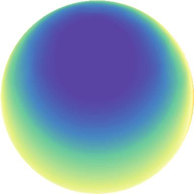
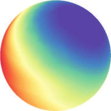
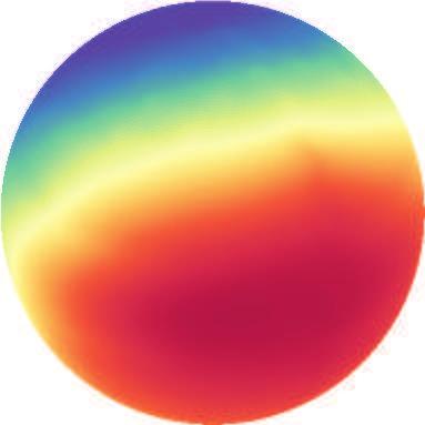
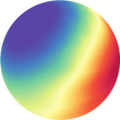
8 A&A 73, A123 (21) Fig. 6. Distribution of the magnetic field on the surface of HD derived from simultaneous MDI analysis of Fe, Nd, and Na. The plots show the distribution of magnetic field modulus (first row), horizontal field (second row), radial field (third row), and field orientation (fourth row) on the surface of HD The bars on the right indicate the field strength in kg. The contours are plotted in steps of 1 kg. The arrow length in the bottom plot is proportional to the field strength. The star is shown at five rotational phases, indicated above the spherical plots Fig. 7. Abundance distribution of Nd, Fe, and Na on the surface of HD The first row shows the surface map of the Nd, the second and third rows illustrate the surface abundance maps of Fe and Na. These maps were derived from the simultaneous mapping of the three elements. The bars on the right next to each panel indicate the abundance in log(nx /Ntot ) units of element X. The contours are plotted with a step of.4 dex Nd and Na, and.2 dex for Fe. The vertical bar indicates the rotation axis. harmonics, containing 96% of the total magnetic field energy. The contribution of all other modes with ` > 2 is much less significant, as shown in Fig. (panel 3). There is a slight asymmetry between the positive (visible) and negative magnetic pole in our final magnetic field maps, see Fig. 6, by approximately.6 kg. This discrepancy probably does not represent sufficient evidence that the magnetic field topology A123, page 8 of 1 of HD deviates strongly from axial symmetry. It might be caused purely by the nature of the magnetic field configuration of the star, where only the positive magnetic pole is visible by an observer from Earth. We conclude that the magnetic field topology of HD has a dominant dipolar component with a very weak contribution at smaller spatial scales from higher-order harmonics. This result

9 N. Rusomarov et al.: Magnetic Doppler Imaging of HD in all four Stokes parameters Stokes I/Ic Relative intensity Fe Fe Fe Fe Fe Fe Nd Nd Nd Na Fe1 68. Fe Fe Fe Fe Fe Fe Fig. 8. Comparison of the observed (dots connected with lines) and synthetic (lines) Stokes I profiles calculated for the final magnetic field and abundance maps (Figs. 7 and 6) for all lines used in the MDI inversion. The distance between two consecutive ticks on the horizontal top axis of each panel is.1 Å, indicating the wavelength scale. Rotational phases are indicated on the right of the figure. contrasts with the finding of a roughly dipole-like global field with strong small-scale features for α2 CVn (Kochukhov & Wade 21) and with the quasi-dipolar field of 3 Cam, which has a mostly dipolar poloidal component with toroidal contributions of similar strength on spatial scales of 3 4 (Kochukhov et al. 24b). The abundance distribution of Fe and Nd for HD was previously derived by Lüftinger et al. (21) from an MDI study of Fe and Nd lines using only Stokes I and V parameters. The new maps confirm these findings and also show some details the previous study lacked. The abundance distribution of Fe varies between.3 and 4.86 dex on the log(nx /Ntotal ) scale. One new detail is the appearance of a roughly circular area around the positive magnetic pole that is strongly depleted relative to the median value by about.3 dex. The new Nd abundance map shows significantly stronger variations that change from 8.66 to 6.4 dex. This corresponds to a range of values of 2.61 dex versus the 1.1 dex reported by Lüftinger et al. (21). The range of the abundance values for Fe is.67 dex and matches the range reported in the previous study. We also found a discrepancy in the location of the Nd spot. Lüftinger et al. (21) detected a possible longitudinal offset, amounting to.4 of the rotation period, of the position of the maximum of the Nd abundance map relative to the maximum of the magnetic field. Our MDI study shows that the longitudinal offset for Nd is very small, if present at all. We attribute this to the better quality of our observational material and the denser phase sampling, resulting in a higher accuracy when determining longitudinal position of abundance spots; Lüftinger et al. (21) could determine longitudinal positions of abundance structures with a precision of.2. rotational periods. We also found that our adopted period, which is slightly shorter than the period used by Lüftinger et al. (21), results in a positive longitudinal shift of about.1 rotational periods relative to the previous study. Therefore, the lack of a visible longitudinal offset of the maximum of the Nd abundance map relative to the position of the maximum of the magnetic field in this work might be caused by a combination of the higher quality of the observations and the revised rotational period used here. The abundance distribution maps of Fe and Nd (Fig. 7) in combination with the magnetic field maps (Fig. 6) reproduce the Stokes profiles of the spectral lines reasonably well. However, there are certain discrepancies in minor spectral details. This can be seen in the Stokes I line profiles of Fe Å. This line has a simple Zeeman-splitting pattern and is highly sensitive to the magnetic field, which results in the appearance of two partially resolved components that are easily visible in the observed A123, page 9 of 1

10 A&A 73, A123 (21) Stokes Q/Ic Relative polarization, % Fe Fe Fe Fe Fe Fe Nd Nd Nd Na Fe1 68. Fe Fe Fe Fe Fe Fe Fig. 9. Same as Fig. 8 for the Stokes Q profiles. Stokes I profiles (Fig. 8), but the synthetic line profiles do not show this splitting. The second example with a similar behavior is the Fe Å line, for which the code 1 does not produce the characteristic splitting in the Stokes I profiles either. Another discrepant behavior is observed in the Stokes Q profiles of the Nd lines, for which the code 1 cannot reproduce the blue wing of the profiles around the maximum of the magnetic field. This problem persists even for an MDI inversion using only Nd lines, although the discrepancy is less pronounced. These discrepancies probably do not affect our results significantly. For the Fe lines with visible Zeeman splitting in the Stokes I profiles, their general behavior with phase is reproduced on a satisfactory level. The observed behavior in the calculated Stokes Q profiles of the Nd lines can be caused by the Stokes Q profiles of Fe lines, which are systematically weaker and more numerous than Nd line profiles (13 versus 3) and thus contribute more to the MDI solution. For the first time for HD 24712, we here attempted to derive an abundance map of Na. The resulting abundance map explains the behavior of Na lines fairly well, whose profiles change in anti-phase to Nd lines. The abundance map of this element shows a strong horizontal gradient, its range of values is 3.49 dex and changes from 8.6 to.16 dex. The morphological characteristics of the Na abundance map contrasts with A123, page 1 of 1 the map for Nd ; Na is overabundant near the negative magnetic pole, which is invisible to the observer from Earth, and is depleted near the positive magnetic pole. This abundance distribution of Na explains the peculiar behavior of the circular polarization profile of the Na Å line, which changes sign around zero phase. However, special care has to be taken when interpreting these results. In Figs we see that our best fit for this line does not properly describe its behavior around zero phase corresponding to magnetic maximum. Our further analysis of this line showed that to fully reproduce the behavior of the line profiles of Na Å with phase, we need to allow the code 1 to produce an abundance map with a range of values of.6 dex instead of with the 3. dex for the map presented in Fig. 7. For such an abundance map the regularization parameter Λa is non-optimal (see Sect. 3.1). We suspect that the reason for the insufficiently good fit of the Na line might be the strong vertical stratification that is made even more complex by NLTE effects. In our current version of the code 1 we do not account for these effects. We plan to investigate vertical stratification structures in a future paper Dipolar field parameters In Paper I we considered our longitudinal magnetic field and net linear polarization measurements inferred from the LSD profiles

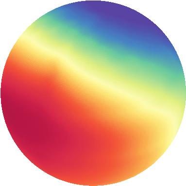
11 N. Rusomarov et al.: Magnetic Doppler Imaging of HD in all four Stokes parameters Stokes U/Ic Relative polarization, % Fe Fe Fe Fe Fe Fe Nd Nd Nd Na Fe1 68. Fe Fe Fe Fe Fe Fe Fig. 1. Same as Fig. 8 for the Stokes U profiles. of HD together with available broad-band linear polarization measurements obtained by Leroy (199) in the framework of the so-called canonical model introduced by Landolfi et al. (1993), and derived the global magnetic field parameters for a purely dipolar magnetic field geometry. The global field parameters agreed well with the previous result obtained by Bagnulo et al. (199), with the exception of a somewhat lower B p obtained by us. Because in this work we used a spherical harmonics decomposition of the magnetic field, it is possible to use the coefficients of the decomposition that correspond to the poloidal field for ` = 1 to derive the dipole field strength B p and the angle β between the rotation axis and the magnetic axis. Using this approach, we derived B p = 3439 G and β = 16 from the solution that was computed from the simultaneous mapping of Fe, Nd, and Na. The comparison of the newly derived values for the dipolar magnetic field parameters with the values presented in Paper I shows that the new value for B p is within three sigma of the previous measurement; the slightly higher value of β by about 1 relative to its previous value may be related to the revised value for the inclination angle i = 12 we adopted here (see Sect. 3.4). We emphasize that the values for B p and β were derived using only a subset of the spherical harmonics coefficients derived in our study and therefore represent a simplified picture of the magnetic field of HD Stokes profiles and surface distribution of calcium Lüftinger et al. (21) attempted to use their magnetic field maps to derive abundance distribution of Ca, but because of limitations of the observational data, they were unable to derive results of any significance. Our unique observational data set opens new possibilities of investigating the abundance distribution for Ca. This element was studied by Ryabchikova et al. (1997) and was used by Shulyak et al. (29) for their vertical stratification analysis, which showed that Ca has a vertical stratification profile similar to that of Fe. It is of particular interest to see how our magnetic field maps reproduce the spectral features of a chemical element with previously unknown abundance distribution. The Ca lines of HD are well suited for this purpose. The line list of Ca lines, shown in Table 2, was composed on basis of the same principles as discussed in Sect. 3.3 the Ca lines were selected based on their phase variations, polarization signatures, and lack of blending by other spectral lines. We used the magnetic field maps (Fig. 6) from the simultaneous MDI study of Fe, Nd, and Na as fixed parameters and derived abundance distribution of Ca. The resulting map for Ca is shown in Fig. 12. The computed and observed Ca line profiles are compared in Fig. 13, which shows that most polarization signatures in the Stokes QUV profiles are reproduced satisfactorily. There are some exceptions in the Stokes I profiles for several lines, in particular for Ca Å and Ca Å. A123, page 11 of 1

12 A&A 73, A123 (21) Stokes V /Ic Relative polarization, % Fe Fe Fe Fe Fe Fe Nd Nd Nd Na Fe1 68. Fe Fe Fe Fe Fe Fe Fig. 11. Same as Fig. 8 for the Stokes V profiles Fig. 12. Abundance distribution of Ca on the surface of HD The bar on the far right denotes the abundance in log(nca /Ntot ) units. The contours are plotted with steps of.4 dex. The vertical bar in each projection indicates the rotation axis. Phase is indicated in the upper right corner of each projection. Table 2. Atomic data of spectral lines used for the MDI inversion of calcium. Ion Ca Ca Ca Ca Ca λ (Å) Elo (ev) log g f.24.9a 1.286a a Notes. Same as Table 1 for the Ca line list. This might be caused by an inhomogeneous vertical distribution of Ca in the atmosphere of HD A123, page 12 of 1 The abundance map of Ca varies across the stellar surface between.4 dex and 7.1 dex. Interestingly, Ca shows an overabundance area close to the magnetic equator and a roughly circular patch at the visible magnetic pole where Ca is depleted relative to its median value. From the comparison of Figs. 7 and 12 we see that this coincides with the abundance map of Fe, which has a similar circular patch around the visible magnetic pole, where Fe is underabundant. One should be careful when interpreting these results because some Ca and Fe lines can be influenced by vertical stratification. It is possible that the roughly circular underabundance patches at the location of the visible magnetic pole derived in our MDI inversions are an artifact caused by ignoring vertical stratification.