Computer Assignment (CA) No. 11: Autocorrelation And Power Spectral Density

Transcription

1 Computer Assignment (CA) No. 11: Autocorrelation And Power Spectral Density Problem Statement Recall the autocorrelation function is defined as: N 1 R(τ) = n=0 x[n]x[n τ],τ = 0, 1, 2,..., M Compute and plot the autocorrelation function for the following signals, and then plot the power spectral density by computing the Fourier transform of the autocorrelation function. 1. Gaussian white noise: N=100, M= An impulse function, : N = 100, M= A periodic impulse train with a period of 20 samples: N = 200, M = A sinewave with a period of 20 samples: N = 200, M = Repeat no. 4 for N = 14, 17, 20, 23, 26. Analyze the behavior that you observe and relate it to the period of the signal. 6. The sum of (1) and (4) at an SNR of 10 db (assume the sinewave is the signal and the Gaussian white noise is the noise): N = 200, M = 60. Explain what you observe. Approach and Results The autocorr() and generate_sine() functions were first reconstructed as can be seen below. The numpy and scipy libraries were also loaded, and a plot style was applied because it looks awesome. The power spectral density is considered, where F[... ] is the fourier transform. F[ R xx (τ)] = S xx (ω)

2 In [7]: %pylab inline from scipy.stats import norm plt.style.use('bmh') def generate_sine(freq, duration, fs, snr): # freq: pure signal frequancy of duration with sample rate fs # and signal to noise ratio snr in db. samples = fs*duration # number of samples is equal to the samples p er second * the number of seconds t = np.linspace(0, duration, samples) # generate time vector freq_radians = (2*np.pi)*freq x = np.sin(freq_radians*t) # generate signal e = norm.rvs(size=samples) c = sqrt(np.var(x)/(np.var(e)*10**(snr/20))) print 20*log(var(x)/var(c*e))/log(10) return x + c*e def autocorr(x, M): ''' Autocorrlates signal X with a delay of M samples. Returns $R_{xx}(t, t-\tau). The function autocorrlated in indexe d past the lag point. ''' Ryy = zeros(m+1) for tau in range(m+1): #print x[m:] #print x[m-tau:-tau] Ryy[tau] = sum( x[m:]*x[m-tau:len(x)-tau] ) return Ryy Populating the interactive namespace from numpy and matplotlib Task 1 N(t) S NN (ω) = c ω 0 E[N(t)] = 0 White noise is defined as a random signal which is normally distributed, contains a flat power spectral density ( for all ) and an expected value of, ( ). The autocorrelation of white noise is calculated as follows, R NN (t, t τ) = E[N(t)N(t τ)], but as every sample in white noise is independent, white noise should result in an autocorrelation of zero for every value except when τ = 0. Further, when τ = 0, the autocorrelation of N(t) becomes the E[N(t ) 2 ], and with E[N(t)] = 0 the autocorrelation becomes R NN (τ) = σn 2 δ(τ) τ = 0 Strangely, this is not exactly what appears in the plot below. The autocorrelation does spike when, but the autocorrelation does not appear to be diminishing as the lag increases. Instead, it fluctuates around the predicted value. The power spectral density of white noise should result in a uniform distribution. The plot after R xx power spectal density, and it is not flat. This is likely due to the limited sample size. S xx (ω) displays the the

3 In [14]: # 1) White Noise Out[14]: (0, 300) N = 100 M = 20 x = norm.rvs(size=n) Rxx = autocorr(x, M) ax = subplot(111) ax.plot(range(m+1), Rxx, label=r"$r_{xx}(\tau)$") ax.set_xlabel(r"$\tau$") ax.legend() fuck = fft.rfft(rxx, n=8192) plot(abs(fuck), label=r"$s_{xx}(\omega)$") xlabel("frequency") legend() ylim([0, 300])

4 Task 2 The autocorrelation of an impulse response,, is displayed below. As the plot illustrates, the autocorrelation is zero for all of. The calculation for the autocorrelation of is as follows: τ x(t) = δ(t 10) Note that when, in other words when, there should be an impulse! The fourier transform of the autocorrelation will, therefore, be uniform for all frequency content. This is displayed in the second plot below. x(t) R xx (t, t τ) = E[δ(t 10)δ(t 10 τ)] t 10 = t 10 τ = 0 τ = 0 In [15]: # 2) Impulse Response N = 100 M = 30 x = 80*[0] + [1] + 9*[0] print x x = array(x) Rxx = autocorr(x, M) print Rxx ax = subplot(111) ax.plot(range(m+1), Rxx, label=r"$r_{xx}(\tau)$") ax.set_xlabel(r"$\tau$") ax.legend() fuck = fft.rfft(rxx, n=8192) plot(abs(fuck), label=r"$s_{xx}(\omega)$") xlabel("frequency") legend()

5 [0, 0, 0, 0, 0, 0, 0, 0, 0, 0, 0, 0, 0, 0, 0, 0, 0, 0, 0, 0, 0, 0, 0, 0, 0, 0, 0, 0, 0, 0, 0, 0, 0, 0, 0, 0, 0, 0, 0, 0, 0, 0, 0, 0, 0, 0, 0, 0, 0, 0, 0, 0, 0, 0, 0, 0, 0, 0, 0, 0, 0, 0, 0, 0, 0, 0, 0, 0, 0, 0, 0, 0, 0, 0, 0, 0, 0, 0, 0, 0, 1, 0, 0, 0, 0, 0, 0, 0, 0, 0] [ ] Out[15]: <matplotlib.legend.legend at 0x7fdabb9ad610>

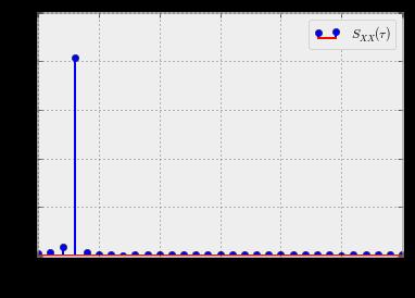
6 Task 3 The autocorrelation of an impulse train also know as the Dirac Comb, T in this case is 20 returns an impulse train with an identical period. This can be seen in the first plot below. R yy This signal will deliver a value when x(t) = n= δ(t nt) where the period (t, t τ) = E[ δ(t nt) δ(t τ kt)] = E[δ(t nt)δ(t τ kt)] n= k= t nt = t τ kt = 0 n= k= t nt (t τ kt) = 0 = τ + (k n)t = 0 k n τ T As and are integers, must be equal to a multiple of the period for the expected value to have any value. This, in turn, would generate an impulse train with an identical period to that of x(t). The fourier transform of the autocorrelation function will also generate an impulse train as proven in signals. This can be seen in the second plot below. In [16]: # 3) Impulse Train with period of 20, N = 200, M = 60 x = [1] + [0]*19 x = 10*x x = np.array(x) M = 60 Rxx = autocorr(x, M) ax = fig.add_subplot(111) ax.stem(range(m+1), Rxx, label=r"$r_{xx}(\tau)$") ax.set_xlabel(r"$\tau$") ax.legend() FFTsig = fft.rfft(rxx, n=128) plot(abs(fftsig), label=r"$s_{xx}(\omega)$") xlabel("frequency") legend()

7 Out[16]: <matplotlib.legend.legend at 0x7fdabc473f50>

8 Task 4 The autocorrelation of a sine wave, identical period and an amplitude equal to the autocorrelation of a continous sine. The expected value of x(t) = a sin(wt) 140/2, returns a sine wave as illustrated by the plot below with an. Explaining this value was an interesting journey. First, I examined R xx (t, t τ) = a 2 a E[sin(u) sin(u 2 τ)] = E[cos(u (u τ)) cos(u + u τ)] 2 cos a (t, t 2 R xx τ) = 2 t for all values of is zero leaving, E[cos(τ) cos(2u τ)] a (t, t 2 R xx τ) = cos(τ) 2... but, then I cried because everything we do is digital and our equation for autocorrelation is reaaaaallllly this. R[n, n τ] = N 1 n=0 x[n]x[n τ],τ = 0, 1, 2,..., M thus N 1 a 2 R xx [n, n τ] = n=0 sin(ωn) sin(ω(n τ)),τ = 0, 1, 2,..., M lets assume a 2 = 1 for simplicity. The trigonometry still holds from the continous example. N 1 1 R xx [n, n τ] = 2 n=0 (cos(ωτ) cos(2ωn τ)),τ = 0, 1, 2,..., M The summation of cos(2ωn τ) will average to zero, leaving N 1 1 N R xx [τ] = cos(ωτ) = cos(ωτ). 2 n=0 2 Wait a second! That still is not equal to 70. Your signal is 200 samples long! What is this 70 giberish. I know this had me up a tree. The signal is 200 samples in length, therefore to calculate the autocorrelation, the function starts the summations at the lag value to ensure the calculation will remain in the bounds of the vector. Therefore, despite taking the autocorrelation of signal that is 200 samples long, the result is the autocorrelation of a signal N M samples long, and, therefore, the amplitude of the signal after autocorrelation is. S XX (ω) will contain a single impulse as the frequency content of second plot below. R XX (τ) (N M)/2 = 70 is at one frequency. This is proven in the

9 In [18]: # 4) A sinewave with a period of 20 samples: N = 200, M = 60. N = 200 M = 60 t = np.arange(n) y = sin(2*pi/20*t) Ryy = autocorr(y, M) ax = fig.add_subplot(111) ax.plot(range(m+1), Ryy, label=r"$r_{xx}(\tau)$") ax.set_xlabel(r"$\tau$") ax.legend() FFTsig = fft.rfft(ryy, n=60) stem(abs(fftsig), label=r"$s_{xx}(\omega)$") xlabel("frequency") legend() Out[18]: <matplotlib.legend.legend at 0x7fdabbcac190>

10 Task 5 Utilizing the reduction quirk of the autocorrelation function, was reduced for the following signals. As calculated N for task 4, the amplitude of the resulting waveform is equal to. 2 S XX (ω) N would be equal to the PSD for task 4 as the signals are identical. The only variation is the amplitude; therefore, the magnitude of the impulses would differ. N In [15]: # 4) Repeat no. 4 for N = 14, 17, 20, 23, 26. # Analyze the behavior that you observe and relate it to the period o f the signal. N = [14, 17, 20, 23, 26] M = 60 t = np.arange(200) y = sin(2*pi/20*t) for n in N: Ryy = autocorr(y, n) ax = fig.add_subplot(111) ax.plot(ryy[0:60], label=r"$r_{yy}[\tau]$, $N = %d$" %(n)) ax.legend() ax.set_xlabel(r"$\tau$") Out[15]: <matplotlib.text.text at 0x7f8d2e75b410>

11 Task 6 As displayed also in computer assignment 9, the autocorrelation of a signal containing white noise filters out a portion of the noise. x a n If representes the sine wave, is a scaler, and is a white noise signal, the output signal can be represented in the following form: y = x + a n. The autocorrelation of the signal would be equal to R yy (τ) = R xx (τ) + a R xn (τ) + a R nx (τ) + a 2 R nn (τ), x(t) n(t) R xn R nx but as and are independent, their crosscorrelation ( and ) is equal to a product of their means which is equal to zero, reducing the autocorrelation sum to R yy (τ) = R xx (τ) + a 2 R nn (τ) Luckily, the autocorrelation of white noise is zero except when the lag value is equal to zero, thus R nn (τ) = R nn (τ)δ(τ) σn 2 δ(τ) E[n(t)] = 0 which simplifies to as the. This results in the final expression for the autocorrelation for output signal with a specific SNR: R yy (τ) = R xx (τ) + a 2 σn 2 δ(τ). The amplitude of the waveform after the spike from the noise when is equal to 0 appears to be identical to that of the signal in task 4 which is predicted by the equation above. The power spectual density will be equal to an impulse at the frequency of the original signal. τ In [21]: N = 200 M = 60 p = 10 x = generate_sine(p, N, 1, 20) plot(x, label=r"x(t)") legend() xlabel("samples") Rxx = autocorr(x, M) ax = fig.add_subplot(111) ax.plot(range(m+1), Rxx, label=r"$r_{xx}(\tau)$") ax.set_xlabel(r"$\tau$") ax.legend() FFTsig = fft.rfft(rxx, n=60) stem(abs(fftsig), label=r"$s_{xx}(\tau)$") xlabel("frequency") legend()

12 20.0 Out[21]: <matplotlib.legend.legend at 0x7fdabba0f710>

13 Conclusions τ > 0 Through the derivations, it has been displayed that autocorrelation cancels any non periodic signals, when. Application of the theory provides slightly different results. For example, the autocorrelation of white noise should result in only a single impulse at τ = 0. Instead, our discrete computations of autocorrelation of white noise provided an impulse at τ = 0 followed by what appears to be random noise at a much lower amplitude centered around a zero. When white noise is added to the sine wave at a low SNR, autocorrelation does not recover the original signal without distortion. I'm not quite sure why in discrete application these phenomenons occur. The limited resolution of digital signals could be the reason.