arxiv: v5 [math.gr] 2 Dec 2014

Transcription

1 Hyperbolically embedded subgroups and rotating families in groups acting on hyperbolic spaces F. Dahmani, V. Guirardel, D. Osin arxiv: v5 [math.gr] 2 Dec 2014 Abstract We introduce and study the notions of hyperbolically embedded and very rotating families of subgroups. The former notion can be thought of as a generalization of the peripheral structure of a relatively hyperbolic group, while the later one provides a natural framework for developing a geometric version of small cancellation theory. Examples of such families naturally occur in groups acting on hyperbolic spaces including hyperbolic and relatively hyperbolic groups, mapping class groups, Out(F n ), and the Cremona group. Other examples can be found among groups acting geometrically on CAT (0) spaces, fundamental groups of graphs of groups, etc. We obtain a number of general results about rotating families and hyperbolically embedded subgroups; although our technique applies to a wide class of groups, it is capable of producing new results even for well-studied particular classes. For instance, we solve two open problems about mapping class groups, and obtain some results which are new even for relatively hyperbolic groups. Contents 1 Introduction 3 2 Main results Hyperbolically embedded subgroups Rotating families Examples Group theoretic Dehn filling Applications Preliminaries General conventions and notation Hyperbolic spaces and group actions Relative presentations and isoperimetric functions Generalizing relative hyperbolicity Weak relative hyperbolicity and bounded presentations

2 4.2 Isolated components in geodesic polygons Paths with long isolated components Hyperbolically embedded subgroups Projection complexes and geometrically separated subgroups Very rotating families Rotating families and windmills Definitions and main results Windmills and proof of the structure theorem Greendlinger s lemmas Quotient space by a very rotating family, hyperbolicity, isometries, and acylindricity Hyperbolic cone-off Examples WPD elements and elementary subgroups Hyperbolically embedded virtually free subgroups Combination theorems Rotating families from small cancellation subgroups Back and forth Some particular groups Dehn filling Dehn filling via rotating families Diagram surgery The general case Applications Largeness properties Subgroups in mapping class groups and Out(F n ) Inner amenability and C -algebras Some open problems 143 Bibliography 145 Index 155 2

3 1 Introduction The notion of a hyperbolic space was introduced by Gromov in his seminal paper [67] and since then hyperbolic geometry has proved itself to be one of the most efficient tools in geometric group theory. Gromov s philosophy suggests that groups acting nicely on hyperbolic spaces have properties similar to those of free groups and fundamental groups of closed hyperbolic manifolds. Of course not all actions, even free ones, are equally good for implementing this idea. Indeed every group G acts freely on the complete graph with G vertices, which is a hyperbolic space. Thus, to derive meaningful results, one needs to impose certain properness conditions. Groups acting on hyperbolic spaces geometrically (i.e., properly and cocompactly) constitute the class of hyperbolic groups. Replacing properness with its relative analogue modulo a fixed collection of subgroups leads to the notion of a relatively hyperbolic group. These classes turned out to be wide enough to encompass many examples of interest, while being restrictive enough to allow building an interesting theory, main directions of which were outlined by Gromov [67]. On the other hand, there are many examples of non-trivial actions of non-relatively hyperbolic groups on hyperbolic spaces: the action of the fundamental group of a graph of groups on the corresponding Bass-Serre tree, the action of the mapping class group of a closed oriented surface on the curve complex, and the action of the outer automorphism group of a free group on the free factor (or free splitting) complex, just to name a few. In general, these actions are very far from being proper. Nevertheless, they can be (and were) used to prove interesting results. The main goal of this paper is to suggest a general approach which allows to study hyperbolic and relatively hyperbolic groups, examples mentioned in the previous paragraph, and many other classes of groups acting on hyperbolic spaces in a uniform way. To achieve this generality, we have to sacrifice global properness (in any reasonable sense). Instead we require the actions to satisfy a properness-like condition that only applies to a selected collection of subgroups. We suggest two ways of formalizeing this idea. The first way leads to the notion of a hyperbolically embedded collection of subgroups, which can be thought of as a generalization of the peripheral structure of relatively hyperbolic groups. The other formalization is based on Gromov s rotating families [68] of special kind, which we call very rotating families of subgroups; they provide a suitable framework to study collections of subgroups satisfying small cancellation conditions. At first glance, these two ways seem quite different: the former is purely geometric, while the latter has rather dynamical flavor. However, they turn out to be closely related to each other and many general results can be proved using either of them. On the other hand, each approach has its own advantages and limitations, so they are not completely equivalent. Groups acting on hyperbolic spaces provide the main source of examples in our paper. Loosely speaking, we show that if a group G acts on a hyperbolic space X so that the action of some subgroup H G is proper, orbits of H are quasi-convex, and distinct translates 3

4 of H-orbits quickly diverge, then H is hyperbolically embedded in G. If K H is a normal subgroup of H and all nontrivial elements of K act on X with large translation length, then the set of conjugates of K in G forms a very rotating family. The main tools used in the proofs of these results are the projection complexes introduced in a recent paper by Bestvina, Bromberg, and Fujiwara [23] and the hyperbolic cone-off construction suggested by Gromov in [68]. This general approach allows us to construct hyperbolically embedded subgroups and very rotating families in many particular classes of groups, e.g., hyperbolic and relatively hyperbolic groups, mapping class groups, Out(F n ), the Cremona group, many fundamental groups of graphs of groups, groups acting properly on proper CAT (0) spaces and containing rank one isometries, etc. Many results previously known for hyperbolic and relatively hyperbolic groups can be uniformly reproved in the general context of groups with hyperbolically embedded subgroups, and very rotating families often provide the most convenient way of doing that. As an illustration of this idea we generalize the group theoretic analogue of Thurston s hyperbolic Dehn surgery theorem proved for relatively hyperbolic groups by the third-named author in [119] (and independently by Groves and Manning [71] in the particular case of finitely generated and torsion free relatively hyperbolic groups). This and other general results from our paper have many particular applications. Despite its generality, our approach is capable of producing new results even for well-studied particular classes of groups. For instance, we answer two well-known questions about normal subgroups of mapping class groups. We also show that the sole existence of a non-degenerate (in a certain precise sense) hyperbolically embedded subgroup in a group G imposes strong restrictions on the algebraic structure of G, complexity of its elementary theory, the structure of operator algebras associated to G, etc. However, we stress that the main goal of this paper is to build a general theory for the future use rather than to consider particular applications. Some further results can be found in [7, 36, 89, 90, 99, 105, 117]. The paper is organized as follows. In the next section we provide a detailed outline of the paper and discuss the main definitions and results. We believe it useful to state most results in a simplified form there, as in the main body of the paper we stick to the ultimate generality which makes many statements rather technical. Section 3 establishes notation and recalls some well-known results used throughout the paper. In Sections 4 and 5 we develop a general theory of hyperbolically embedded subgroups and rotating families, respectively. Most examples are collected in Section 6. Section 7 is devoted to the proof of the Dehn filling theorem. Applications are collected in Section 8. Finally we discuss some open questions and directions for the future research in Section 9. Acknowledgments. We are grateful to Mladen Bestvina, Brian Bowditch, Montse Casals- Ruiz, Remi Coulon, Thomas Delzant, Pierre de la Harpe, Ilya Kazachkov, Ashot Minasyan, Alexander Olshanskii, Mark Sapir, and Alessandro Sisto with whom we discussed various topics related to this paper, and to the referee. We benefited a lot from these discussions. The first two authors were partially supported by the ANR grant ANR 2011-BS and the IUF. The research of the third author was supported by the NSF grants DMS , DMS , and by the RFBR grant

5 2 Main results 2.1 Hyperbolically embedded subgroups The first key concept of our paper is the notion of a hyperbolically embedded collection of subgroups. For simplicity, we only discuss the case when the collection consists of a single subgroup here and refer to Section 4 for the general definition. Let G be a group, H a subgroup of G, X a (not necessary finite) subset of G. If G = X H, we denote by Γ(G, X H) the Cayley graph of G with respect to the generating set X H. Here we think of X and H as disjoint alphabets; more precisely, disjointness of the union X H means that if some x X and h H represent the same element g G, then Γ(G, X H) contains two edges connecting every vertex v G to the vertex vg: one edge is labelled by x and the other is labelled by h. Let also Γ H denote the Cayley graph of H with respect to the generating set H. Clearly Γ H is a complete subgraph of Γ(G, X H). We say that a path p in Γ(G, X H) is admissible if p does not contain edges of Γ H. Note that we do allow p to pass through vertices of Γ H. Given two elements h 1, h 2 H, define d(h 1, h 2 ) to be the length of a shortest admissible path p in Γ(G, X H) that connects h 1 to h 2. If no such path exists we set d(h 1, h 2 ) =. Since concatenation of two admissible paths is an admissible path, it is clear that d: H H [0, ] is a metric on H. (For the triangle inequality to make sense we extend addition from [0, ) to [0, ] in the obvious way.) Definition 2.1. We say that H is hyperbolically embedded in G with respect to a subset X G (and write H h (G, X)) if the following conditions hold. (a) G is generated by X H. (b) The Cayley graph Γ(G, X H) is hyperbolic. (c) (H, d) is a proper metric space, i.e., every ball (of finite radius) is finite. We also say that H is hyperbolically embedded in G (and write H h G) if H h (G, X) for some X G. Example 2.2. (a) Let G be any group. Then G h G. Indeed take X =. Then the Cayley graph Γ(G, X H) has diameter 1 and d(h 1, h 2 ) = whenever h 1 h 2. Further, if H is a finite subgroup of a group G, then H h G. Indeed H h (G, X) for X = G. These cases are referred to as degenerate. In what follows we are only interested in non-degenerate examples. (b) Let G = H Z, X = {x}, where x is a generator of Z. Then Γ(G, X H) is quasiisometric to a line and hence it is hyperbolic. However d(h 1, h 2 ) 3 for every h 1, h 2 H. Indeed in the shift xγ H of Γ H there is an edge (labelled by h 1 1 h 2 H) connecting h 1 x to h 2 x, so there is an admissible path of length 3 connecting h 1 to h 2 (see Fig. 1). Thus if H is infinite, then H h (G, X). Moreover it is not hard to show that H h G. (c) Let G = H Z, X = {x}, where x is a generator of Z. In this case Γ(G, X H) is quasiisometric to a tree (see Fig. 1) and d(h 1, h 2 ) = unless h 1 = h 2. Thus H h (G, X). 5

6 x x x xγ H xγ H... x x x... h 1 h 2 Γ H 1 Γ H x x x... x x x x 1 Γ H x 1 Γ H Figure 1: Cayley graphs Γ(G, X H) for G = H Z and G = H Z. Our approach to the study of hyperbolically embedded subgroups is inspired by [120]. In particular, we first provide an isoperimetric characterization of hyperbolically embedded subgroups, which resembles the corresponding characterization of relatively hyperbolic groups. Recall that a relative presentation of a group G with respect to a subgroup H G and a subset X G is a presentation of the form G = H, X R, (1) which is obtained from a presentation of H by adding the set of generators X and the set of relations R. Thus G = H F (X)/ R, where F (X) is the free group with basis X and R is the normal closure of R in H F (X). The relative presentation (1) is bounded, if all elements of R have uniformly bounded length being considered as words in the alphabet X H; further it is strongly bounded if, in addition, the set of letters from H appearing in words from R is finite. For instance, if H is an infinite group with a finite generating set A, then the relative presentation H, {x} [x, h] = 1, h H of the group G = H Z is bounded but not strongly bounded. presentation H, {x} [a, x] = 1, a A of the same group is strongly bounded. On the other hand, the The relative isoperimetric function of a relative presentation is defined in the standard way. Namely we say that f : N N is a relative isoperimetric function of a relative presentation 6

7 (1), if for every n N and every word W of length at most n in the alphabet X ±1 H which represents the trivial element in G, there exists a decomposition W = k fi 1 R i ±1 f i i=1 in the free product H F (X), where for every i = 1,..., k, we have f i H F (X), R i R, and k f(n). Theorem 2.3 (Theorem 4.24). Let G be a group, H a subgroup of G, X a subset of G such that G = X H. Then H h (G, X) if and only if there exists a strongly bounded relative presentation of G with respect to X and H with linear relative isoperimetric function. This theorem and the analogous result for relatively hyperbolic groups (see [120]) imply that the notion of a hyperbolically embedded subgroup indeed generalizes the notion of a peripheral subgroup of a relatively hyperbolic group, where one requires X to be finite. More precisely, we have the following. Proposition 2.4 (Proposition 4.28). Let G be a group, H G a subgroups of G. Then G is hyperbolic relative to H if and only if H h (G, X) for some (equivalently, any) finite subset X of G. On the other hand, by allowing X to be infinite, we obtain many other examples of groups with hyperbolically embedded subgroups. A rich source of such examples is provided by groups acting on hyperbolic spaces. More precisely, we introduce the following. Definition 2.5. Let G be a group acting on a space S. Given an element s S and a subset H G, we define the H-orbit of s by H(s) = {h(s) h H}. We say that (the collection of cosets of) a subgroup H G is geometrically separated if for every ε > 0 and every s S, there exists R > 0 such that the following holds. Suppose that for some g G we have diam ( H(s) (gh(s)) +ε) R, where (gh(s)) +ε denotes the ε-neighborhood of the gh-orbit of s in S. Then g H. Informally, the definition says that distinct translates of the H-orbit of s rapidly diverge. It is also fairly easy to see that replacing every s S with some s S yields an equivalent definition (see Remark 4.41). Example 2.6. Suppose that G is generated by a finite set X. Let S = Γ(G, X), and H a subgroup of G. Then geometric separability of H with respect to the natural action on S implies that H is almost malnormal in G, i.e., H g H < for any g / H. (The converse is not true in general.) 7

8 Theorem 2.7 (Theorem 4.42). Let G be a group acting by isometries on a hyperbolic space S, H a geometrically separated subgroup of G. Suppose that H acts on S properly and there exists s S such that the H-orbit of s is quasiconvex in S. Then H h G. This theorem is one of the main technical tools in our paper. In Section 2.3, we will discuss many particular examples of groups with hyperbolically embedded subgroups obtained via Theorem 2.7. To prove the theorem, we first use the Bestvina-Bromberg-Fujiwara projection complexes (see Definition 4.37) to construct a hyperbolic space on which G acts coboundedly. Then a refined version of the standard Milnor-Svarč argument allows us to construct a (usually infinite) subset X G such that H h (G, X). Here we mention just one application of Theorem 2.7, which makes use of the following notion introduced by Bestvina and Fujiwara [27]. Definition 2.8. Let G be a group acting on a hyperbolic space S, h an element of G. One says that h satisfies the weak proper discontinuity condition (or h is a WPD element) if for every ε > 0 and every x S, there exists N = N(ε) such that {g G d(x, g(x)) < ε, d(h N (x), gh N (x)) < ε} <. (2) Recall also that an element h G is loxodromic if the map Z S given by n h n (s) is a quasi-isometric embedding for some (equivalently any) s S. This corollary summarizes Lemma 6.5 and a particular case of Theorem 6.8. To prove it, we verify that H = E(h) satisfies all assumptions of Theorem 2.7. Corollary 2.9. Let G be a group acting on a hyperbolic space and let h be a loxodromic WPD element. Then h is contained in a unique maximal virtually cyclic subgroup of G, denoted E(h), and E(h) h G. Let us mention one restriction which is useful in proving that a subgroup is not hyperbolically embedded in a group. In fact, it is a generalization of Example 2.2 (b). Proposition 2.10 (Proposition 4.33). Let G be a group, H a hyperbolically embedded subgroup of G. Then H is almost malnormal, i.e., H H g < whenever g / H. Yet another obstruction for being hyperbolically embedded is provided by homological invariants. It was proved by the first and the second author [52] that every peripheral subgroup of a finitely presented relatively hyperbolic group is finitely presented. This was generalized by Gerasimov-Potyagailo [65] to a class of quasiconvex subgroups of relatively hyperbolic groups. In this paper we generalize the result of [52] in another direction, namely to hyperbolically embedded subgroups. Our argument is geometric, inspired by [65], and allows us to obtain several finiteness results in a uniform way. It is worth noting that for n > 2 parts b) and c) of Theorem 2.9 below are new even for peripheral subgroups of relatively hyperbolic groups. Recall that a group G is said to be of type F n (n 1) if it admits an Eilenberg-MacLane space K(G, 1) with finite n-skeleton. Thus conditions F 1 and F 2 are equivalent to G being finitely generated and finitely presented, respectively. Further G is said to be of type F P n if the 8

9 trivial G-module Z has a projective resolution which is finitely generated in all dimensions up to n. Obviously F P 1 is equivalent to F 1. For n = 2 these conditions are already not equivalent; indeed there are groups of type F P 2 that are not finitely presented [22]. For n 2, F n implies F P n and is equivalent to F P n for finitely presented groups. For details we refer to the book [37]. Recall also that for n 1, the n-dimensional Dehn function of a group G is defined whenever G has type F n+1 ; it is denoted by δ (n) G. In particular δ(1) G = δ G is the ordinary Dehn function of G. The definition can be found in [5] or [33]; we stick to the homotopical version here and refer to [33] for a brief review of other approaches. As usual we write f g for some functions f, g : N N if there are A, B, C, D N such that f(n) Ag(Bn) + Cn + D for all n N. In Section 4.3, we prove the following. Theorem 2.11 (Corollary 4.32). Let G be a finitely generated group and let H be a hyperbolically embedded subgroup of G. Then the following conditions hold. (a) H is finitely generated. (b) If G is of type F n for some n 2, then so is H. Moreover, we have δ n 1 H particular, if G is finitely presented, then so is H and δ H δ G. δn 1 G. In (c) If G is of type F P n, then so is H. Many other results previously known for relatively hyperbolic groups can be reproved in the general context of hyperbolically embedded subgroups. One of the goals of this paper is to help making this process automatic. More precisely, in Section 4 we generalize some useful technical lemmas originally proved for relatively hyperbolic groups in [119, 120] to the case of hyperbolically embedded subgroups. Then proofs of many results about relatively hyperbolic groups work in the general context of hyperbolically embedded subgroups almost verbatim after replacing references. This approach is illustrated by the proof of the group theoretic analogue of Thurston s Dehn filling theorem discussed in Section Rotating families. The other main concept used in our paper is that of an α-rotating family of subgroups, which we again discuss in the particular case of a single subgroups here. It is based on the notion of a rotating family (or rotation family, or rotation schema), which was introduced by Gromov in [68, 26 28] in the context of groups acting on CAT (κ) spaces with κ 0. It allows to envisage a small-cancellation like property for a family of subgroups in a group through a geometric configuration of a space upon which the group acts and in which the given subgroups fix different points. The essence of this definition is that we have a G-invariant collection of points, and for each point c in this collection, a subgroup G c of G whose non-trivial elements act as rotations around c with a large angle. This angle condition would make sense in a CAT (0) or CAT ( 1) space, and the definition we give mimics this situation in the coarser setting of a Gromov-hyperbolic space (see Figure 2). Because of this coarseness, we need to 9

10 Figure 2: In a very rotating family, g G c \ {1} rotates by a large angle assume that the points c in our family are sufficiently far away from each other compared to the hyperbolicity constant. Definition (a) (Gromov s rotating families) Let G X be an action of a group on a metric space. A rotating family C = (C, {G c, c C}) consists of a subset C X, and a collection {G c, c C} of subgroups of G such that (a-1) C is G-invariant, (a-2) each G c fixes c, (a-3) g G c C G gc = gg c g 1. The set C is called the set of apices of the family, and the groups G c are called the rotation subgroups of the family. (b) (Separation) One says that C (or C) is ρ-separated if any two distinct apices are at distance at least ρ. (c) (Very rotating condition) When X is δ-hyperbolic for some δ > 0, one says that C is very rotating if, for all c C, g G c \ {1}, and all x, y X with both d(x, c), d(y, c) in the interval [20δ, 40δ] and d(gx, y) 15δ, any geodesic between x and y contains c. (d) (α-rotating subgroup) A subgroup H of a group G is called α-rotating if there is an αδ-separated very rotating family of G acting on a δ-hyperbolic space X for some δ > 0 whose rotation subgroups are exactly the conjugates of H. When we want to stress a particular action, we will say that H is α-rotating with respect to the given action of G on X. Example Suppose that G = H K. Let C be the set of vertices of the corresponding Bass-Serre tree X and let G c denote the stabilizer of c C in G. Then we obtain a rotating family C = (C, {G c, c C}) of subgroups of G. Since X is δ-hyperbolic for any δ > 0, we see that H and K are α-rotating subgroups of G for every α > 0. 10

11 These definitions come with three natural problems. First, study the structure of the subgroups generated by rotating families. Second, study the quotients of groups and spaces by the action of rotating families. Third, provide a way to construct spaces with rotating families in different contexts. We will show that the first two questions can be answered for α-rotating collections of subgroups if α is large enough and provide many examples of such collections. The main structural result about rotating families is a partial converse of Example Recall that given a subset S of a group G, we denote by S G the normal closure of S in G, i.e., the minimal normal subgroup of G containing S. Theorem 2.14 (Theorem 5.3). Let G be a group acting on a hyperbolic space X, H an α- rotating subgroup of G with respect to this action for some α 200. Then the following holds. (a) There exists a (usually infinite) subset T G such that H G = t T t 1 Ht. (b) Every element h H G either is conjugate to an element of H, or is loxodromic with respect to the action on X The proof of this result is inspired by [68, 26 28], where X is assumed to be CAT (0). Claiming that this context has rather limited application, Gromov indicates that a generalization to spaces with approximately negative curvature is desirable and sketches it in [70] and [69]. A result similar to Theorem 2.14 was stated in [69, 1/6 theorem]. For the proof, Gromov refers to the Delzant s paper [53], which deals with the particular case of hyperbolic groups. Delzant did not use rotating families there, and his argument, which can indeed be generalized, is quite technical. We propose here an alternative proof inspired by the more geometric settings of [68, 26 28]; our approach is based on the notion of a windmill introduced in Section 5.1. A standard way of producing very rotating families is through a coning-off construction proposed by Gromov [68, 29 32] for CAT (κ) spaces with κ < 0. It was later adapted to approximate negative curvature in [8, 49, 54]. The general idea is to start with some action of a group G on a hyperbolic space and then glue hyperbolic cones to orbits of a family of subgroups to make these subgroups elliptic. In general, this does not yield a very rotating family; in fact, the resulting space may not be even hyperbolic. In order to be able to proceed with the coning-off construction while getting a suitable space, we introduce a condition of small cancellation flavor (see Definition 6.22 and Proposition 6.23). We mention here a particular application of this idea to acylindrical actions and, more generally, group actions with WPD loxodromic elements. Definition Following Bowditch [31], we say that an action of a group G on a metric space X is acylindrical if for any ε 0, there exist R = R(ε) > 0 and N = N(ε) > 0 such that for all x, y X with d(x, y) R, the set contains at most N elements. {g G d(x, gx) ε, d(y, gy) ε} 11

12 It is easy to see that if the action of Γ(G, X H) on X is acylindrical, then every loxodromic element g G is WPD (see Definition 2.8). Thus part (a) of the proposition applies to a more general situation than part (b), while the conclusion in part (b) is more uniform. Proposition 2.16 (Proposition 6.34). Let G be a group acting on a hyperbolic space X and let α be a positive number. (a) For any loxodromic WPD element g G, there exists m = m(α, g) N such that the subgroup g m is α-rotating with respect to the induced action of G on a certain cone-off of X. (b) If the action of G on X is acylindrical, then there exists n = n(α) such that for every loxodromic g G the subgroup g n is α-rotating with respect to the induced action of G on a certain cone-off of X. After obtaining a rotating family acting on a suitable space, one may want to quotient this space by the group normally generated by the very rotating family. A typical result of this type would assert that hyperbolicity is preserved, possibly in an effective way (compare to [69, Theorem 1/7]). This is indeed what we obtain in Propositions 5.28 and In addition, we show that, under certain mild assumptions, acylindricity is preserved through coning-off and taking such a quotient (see Propositions 5.40 and 5.33, respectively). These results can be summarized as follows. Proposition Let G be a group acting on a hyperbolic graph X. Let H be an α-rotating subgroup of G with respect to this action, where α in large enough. Then for any, the following conditions hold. (a) X/ H G is Gromov-hyperbolic (b) The quotient map X X/ H G is a local isometry away from the apices of the rotating family. (c) Any elliptic isometry of X/ H G in G/ H G has a preimage in G that is elliptic. (d) Suppose that the action of G on X is acylindrical. Suppose also that, for a fixed point c of H in X, the action of the stabilizer Stab G (c) on the sphere centered at c satisfies a certain properness assumption (see 5.33). Then the action of G/ H G on X/ H G is acylindrical. Preservation of acylindricity allows us to iterate applications of Corollary 2.16 and Proposition 2.17 infinitely many times and construct some interesting quotient groups (see Section 8.2). 2.3 Examples We now discuss some examples of hyperbolically embedded and α-rotating subgroups. Before looking at particular groups, let us mention one general result, which allows us to pass from hyperbolically embedded subgroups to α-rotating ones. 12

13 Theorem 2.18 (Theorem 6.35). Suppose H is a hyperbolically embedded subgroup of a group G. Then for every α > 0, there exists a finite subset F H \ {1} such that the following holds. Let N H be a normal subgroup of H that contains no elements of F. Then N is an α-rotating subgroup of G. In particular, this theorem together with Proposition 2.4 allows us to construct α-rotating subgroups in relatively hyperbolic groups. Yet another typical application is the case when H is infinite and virtually cyclic. In this case, it is easy to show that for every infinite order element h H and every α > 0, there exists k N such that the subgroup h k is α-rotating (see Corollary 6.37). Below we consider some examples where the groups are not, in general, relatively hyperbolic. The first class of examples consists of mapping class groups. Let Σ be a (possibly punctured) orientable closed surface. The mapping class group MCG(Σ) is the group of isotopy classes of orientation preserving homeomorphisms of Σ; we do allow homeomorphisms to permute the punctures. By Thurston s classification, an element of MCG(Σ) is either of finite order, or reducible (i.e., fixes a multi-curve), or pseudo-anosov. Recall that all but finitely many mapping class groups are not relatively hyperbolic, essentially because of large degree of commutativity [6]. However, we prove the following result (see Theorem 6.50 and Theorem 8.10). Theorem Let Σ be a (possibly punctured) orientable closed surface and let MCG(Σ) be its mapping class group. (a) For every pseudo-anosov element a MCG(Σ), we have E(a) h MCG(Σ), where E(a) is the unique maximal virtually cyclic subgroup containing a. (b) For every α > 0, there exists n N such that for every pseudo-anosov element a MCG(Σ), the cyclic subgroup a n is α-rotating. (c) Every subgroup of MCG(Σ) is either virtually abelian or virtually surjects onto a group with a non-degenerate hyperbolically embedded subgroup. We explain the proof in the case on non-exceptional surfaces. That is, we assume that 3g + p > 4, where g and p are the genus and the number of punctures of Σ, respectively. In all exceptional cases, MCG(Σ) is a hyperbolic group, and the proof is much easier. Associated to Σ is its curve complex C, on which MCG(Σ) acts by isometries; pseudo- Anosov elements of MCG(Σ) are exactly loxodromic elements with respect to this action. Recall that C is hyperbolic for all non-exceptional surfaces Σ [101] and the action of MCG(Σ) on C is acylindrical [31] (the WPD property for pseudo-anosov elements was established earlier in [27]). Thus we obtain (a) by applying Corollary 2.9 to the action of the mapping class group on the corresponding curve complex. We note that the subgroup a is not necessarily hyperbolically embedded. In fact, Proposition 2.10 easily implies that no proper infinite subgroup of E(a) is hyperbolically embedded in MCG(Σ). Further, part (b) follows immediately from Proposition 2.16 (b). Finally, part (c) is easy to derive from (a) and Ivanov s trichotomy, 13

14 stating that every subgroup of a mapping class group is either finite, or reducible, or contains a pseudo-anosov element [92]. A similar result can be proved for the group Out(F n ) of outer automorphisms of a free group. Recall that an element g Out(F n ) is irreducible with irreducible powers (or iwip, for brevity) if none of its non-trivial powers preserve the conjugacy class of a proper free factor of F n. These automorphisms play the role of pseudo-anosov mapping classes in the usual analogy between mapping class groups and Out(F n ). As an analogue of the curve complex, we can use the free factor complex [26], or a specially crafted hyperbolic complex [25] on which a given iwip element g acts loxodromically and satisfies the WPD condition. Arguing as above, we obtain: Theorem 2.20 (Theorem 6.51). Let F n be the free group of rank n, g an iwip element. Then E(g) h Out(F n ), where E(g) is the unique maximal virtually cyclic subgroup of Out(F n ) containing g. Furthermore, for every α > 0, there exists k N such that the cyclic subgroup g k is α-rotating. Remark Note that this theorem is significantly weaker than Theorem There are two reasons: first, currently there is no known hyperbolic space on which Out(F n ) acts acylindrically so that all iwip elements are exactly the loxodromic ones; second, no analogue of Ivanov s trichotomy is known for subgroups of Out(F n ). The recent papers [77, 84] provide another hyperbolic space on which Out(F n ) acts. It is very well possible that further study of the action of Out(F n ) on this or other similar spaces will lead to a stronger version of the theorem. The same argument also works for the group Bir(P 2 C ) of birational transformations of the projective plane P 2 C, called the Cremona group. For the definition and details about Bir(P2 C ) we refer to the survey [39]. In [41], Cantat and Lamy introduced the notion of a tight element (see Definition 6.52) and proved that most elements of Bir(P 2 C ) are tight. They use this notion to prove that the Cremona group is not simple, using a generalization of small cancellation arguments by Delzant [53]. Tight elements act loxodromically on a hyperbolic space naturally associated to Bir(P 2 C ). Existence of tight elements and some additional results from [29, 41] allow us to apply Theorem 2.7 to certain virtually cyclic subgroups containing these elements. Theorem 2.22 (Corollary 6.54). Let g be a tight element of the Cremona group Bir(P 2 C ). Then there exists a virtually cyclic subgroup E(g) of Bir(P 2 C ) which contains g and is hyperbolically embedded in Bir(P 2 C ). Furthermore, for every α > 0, there exists k N such that the cyclic subgroup g k is α-rotating. The next example is due to Sisto [142]. It answers a question from the first version of this paper. Theorem 2.23 (Sisto [142]). Let G be a group acting properly on a proper CAT (0) space. Suppose that g G is a rank one isometry. Then g is contained in a unique maximal virtually cyclic subgroup of G, which is hyperbolically embedded in G. This result also gives rise to rotating families via Theorem The notion of a rank one isometry originates in the Ballman s paper [11]. Recall that an axial isometry g of a CAT (0) space S is rank one if there is an axis for g which does not bound 14

15 a flat half-plane. Here a flat half-plane means a totally geodesic embedded isometric copy of an Euclidean half-plane in S. For details see [12, 76] and references therein. Theorem 2.23 provides a large source of groups with non-degenerated hyperbolically embedded subgroups. For instance let M be an irreducible Hadamard manifold that is not a higher rank symmetric space. Suppose that a group G acts on M properly and cocompactly. Then G always contains a rank one isometry [13, 14, 38]. Conjecturally, the same conclusion holds for any locally compact geodesically complete irreducible CAT (0) space that is not a higher rank symmetric space or a Euclidean building of dimension at least 2 [15]. Recall that a CAT (0) space is called geodesically complete if every geodesic segment can be extended to some bi-infinite geodesic. This conjecture was settled by Caprace and Sageev [43] for CAT (0) cube complexes. Namely, they show that for any locally compact geodesically complete CAT (0) cube complex Q and any infinite discrete group G acting properly and cocompactly on Q, Q is a product of two geodesically complete unbounded convex subcomplexes or G contains a rank one isometry. For instance, this applies to right angled Artin and Coxeter groups acting on the universal covers of their Salvetti complexes and their Davis complexes, respectively (see [46] for details). In most examples discussed above, the hyperbolically embedded subgroups are elementary (i.e. virtually cyclic). The next result allows us to construct non-elementary hyperbolically embedded subgroups starting from any non-degenerate (but possibly elementary) ones. The proof is also based on Theorem 2.7 and a small cancellation like argument. This theorem has many applications, e.g., to the proof of SQ-universality and C -simplicity of groups with non-degenerate hyperbolically embedded subgroups, discussed in Section 2.5. Theorem 2.24 (Theorem 6.14). Suppose that a group G contains a non-degenerate hyperbolically embedded subgroup. Then the following hold. (a) There exists a (unique) maximal finite normal subgroup of G, denoted K(G). (b) For every infinite subgroup H h G, we have K(G) H. (c) For any n N, there exists a subgroup H G such that H h G and H = F n K(G), where F n is a free group of rank n. Given groups with hyperbolically embedded subgroups, we can combine them using amalgamated products and HNN-extensions. In Section 6 we discuss generalizations of some combination theorems previously established for relatively hyperbolic groups by Dahmani [51]. Here we state our results in a simplified form and refer to Theorem 6.19 and Theorem 6.20 for the full generality. The first part of the theorem requires the general definition of a hyperbolically embedded collection of subgroups, which we do not discuss here (see Definition 4.25). Theorem (a) Let G be a group, {H, K} a hyperbolically embedded collection of subgroups, ι : K H a monomorphism. Then H is hyperbolically embedded in the HNN extension G, t t 1 kt = ι(k), k K. (3) 15

16 (b) Let H and K be hyperbolically embedded isomorphic subgroups of groups A and B, respectively. Then H = K is hyperbolically embedded in the amalgamated product A H=K B. Finally we note that many non-trivial examples of hyperbolically embedded subgroups can be constructed via group theoretic Dehn filling discussed in the next section. 2.4 Group theoretic Dehn filling Roughly speaking, Dehn surgery on a 3-dimensional manifold consists of cutting of a solid torus from the manifold (which may be thought of as drilling along an embedded knot) and then gluing it back in a different way. The study of these elementary transformations is partially motivated by the Lickorish-Wallace theorem, which states that every closed orientable connected 3-manifold can be obtained by performing finitely many surgeries on the 3-dimensional sphere. The second part of the surgery, called Dehn filling, can be formalized as follows. Let M be a compact orientable 3 manifold with toric boundary. Topologically distinct ways to attach a solid torus to M are parameterized by free homotopy classes of unoriented essential simple closed curves in M, called slopes. For a slope σ, the corresponding Dehn filling M(σ) of M is the manifold obtained from M by attaching a solid torus D 2 S 1 to M so that the meridian D 2 goes to a simple closed curve of the slope σ. The fundamental theorem of Thurston [145, Theorem 1.6] (see [86, 127] for proofs) asserts that if M \ M admits a complete finite volume hyperbolic structure, then the resulting closed manifold M(σ) is hyperbolic provided σ is not in a finite set of exceptional slopes. Algebraically this means that for all but finitely many primitive elements x π 1 ( M) π 1 (M), the quotient group of π 1 (M) by the normal closure of x (which is isomorphic to π 1 (M(σ)) by the Seifert-van Kampen theorem) is non-elementary hyperbolic. Modulo the geometrization conjecture proved by Perelman, this algebraic statement is equivalent to the Thurston theorem. Dehn filling can be generalized in the context of abstract group theory as follows. Let G be a group and let H be a subgroup of G. One can think of G and H as the analogues of π 1 (M) and π 1 ( M), respectively. Instead of considering just one element x H, let us consider a normal subgroup N H. By N G we denote its normal closure in G. Associated to this data is the quotient group G/ N G, which we call the group theoretic Dehn filling of G. Theorem 2.26 (Osin [119]). Suppose that a group G is hyperbolic relative to a subgroup H. Then for any subgroup N H avoiding a fixed finite set of nontrivial elements, the natural map from H/N to G/ N G is injective and G/ N G is hyperbolic relative to H/N. In particular, if H/N is hyperbolic, then so is G/ N G. This theorem was proved in [119]; an independent proof for finitely generated torsion free relatively hyperbolic groups was later given in [71]. Since the fundamental group of a complete finite volume hyperbolic manifold M with toric boundary is hyperbolic relative to the subgroup π 1 ( M) [61] (which does embed in π 1 (M) in this case), the above result can be thought of as a generalization of the Thurston theorem. 16

17 In this paper we further generalize these results to groups with hyperbolically embedded subgroups. We also study the kernel of the filling and obtain some other results which are new even for relatively hyperbolic groups. We state a simplified version of our theorem here and refer to Theorem 7.19 for a more general and stronger version. Theorem Let G be a group, H a subgroup of G. Suppose that H h (G, X) for some X G. Then there exists a finite subset F of nontrivial elements of H such that for every subgroup N H that does not contain elements from F, the following hold. (a) The natural map from H/N to G/ N G is injective (equivalently, H N G = N). (b) H/N h (G/ N G, X), where X is the natural image of X in G/ N G. (c) Every element of N G is either conjugate to an element of N or acts loxodromically on Γ(G, X H). Moreover, translation numbers of loxodromic elements of N G are uniformly bounded away from zero. (d) N G = t T N t for some subset T G. The proof of parts (a) and (b) makes use of van Kampen diagrams and Theorem 2.3, while parts (c) and (d) are proved using rotating families, namely Theorem 2.18 and Theorem Note that parts (c) and (d) of this theorem (as well as some other parts of Theorem 7.19) are new even for relatively hyperbolic groups. 2.5 Applications We start with some results about mapping class groups. The following question is Problem 2.12(A) in Kirby s list. It was asked in the early 80s and is often attributed to Penner, Long, and McCarthy. It is also recorded by Ivanov [93, Problems 3], and Farb refers to it in [62, 2.4] as a well known open question. Recall that a subgroup of a mapping class group is called purely pseudo-anosov, if all its non-trivial elements are pseudo-anosov. Problem Let Σ be a closed orientable surface. Does MCG(Σ) contain a non-trivial purely pseudo-anosov normal subgroup? The abundance of finitely generated (non-normal) purely pseudo-anosov free subgroups of MCG(Σ) is well known, and follows from an easy ping-pong argument. However, this method does not elucidate the case of infinitely generated normal subgroups. For a surface of genus 2 the problem was answered by Whittlesey [148] who proposed an example based on Brunnian braids (see also the study of Lee and Song of the kernel of a variation of the Burau representation [95]). Unfortunately methods of [148, 95] do not generalize to closed surfaces of higher genus. Another question was probably first asked by Ivanov (see [93, Problem 11]). Farb also recorded this question in [62, Problem 2.9], and qualified it as a basic test question for understanding normal subgroups of MCG(Σ). 17

18 Problem Let Σ be a closed orientable surface. Is the normal closure of a certain nontrivial power of a pseudo-anosov element of MCG(Σ) free? We answer both questions positively. In fact, our approach can be used in more general settings. Namely, we derive the following from Proposition 2.16 and Theorem Part (a) can be alternatively derived from Corollary 2.9 and Theorem Theorem 2.30 (Theorem 8.7). Let G be a group acting on a hyperbolic space X. (a) For every loxodromic WPD element g G, there exists n N such that the normal closure g n in G is free. (b) If the action of G is acylindrical, then there exists n N such that for every loxodromic element g G, the normal closure g n in G is free. Moreover, in both cases every non-trivial element of g n is loxodromic with respect to the action on X. This result can be viewed as a generalization of Delzant s theorem [53] stating that for a hyperbolic group G and every element of infinite order g G, there exists n N such that g n is free (see also [47] for a clarification of certain aspects of Delzant s proof). Applying Theorem 2.30 to mapping class groups acting on the corresponding curve complexes, we obtain: Theorem 2.31 (Theorem 8.8). Let Σ be a (possibly punctured) closed orientable surface. Then there exists n N such that for any pseudo-anosov element a MCG(Σ), the normal closure of a n is free and purely pseudo-anosov. For Out(F n ), we cannot achieve such a uniform result for the reason explained in Remark Newertheless, we obtain the following theorem by applying Theorem 2.30 to the action of Out(F n ) on the free factor complex. Theorem 2.32 (Theorem 8.12). Let f be an iwip element of Out(F n ). n N such that the normal closure of f n is free and purely iwip. Then there exists Using techniques developed in our paper it is not hard to obtain many general results about groups with hyperbolically embedded subgroups. We prove just some of them to illustrate our methods and leave others for future papers. We start with a theorem, which shows that a group containing a non-degenerate hyperbolically embedded subgroup is large in many senses. Recall that the class of groups with non-degenerate hyperbolically embedded subgroups includes non-elementary hyperbolic and relatively hyperbolic groups with proper peripheral subgroups, all but finitely many mapping class groups, Out(F n ) for n 2, the Cremona group, and many other examples. Theorem 2.33 (Theorem 8.1). Suppose that a group G contains a non-degenerate hyperbolically embedded subgroup. Then the following hold. 18

19 (a) The group G is SQ-universal. Moreover, for every finitely generated group S there is a quotient group Q of G such that S h Q. (b) dim H 2 b (G, R) = 1 In particular, G is not boundedly generated. (c) The elementary theory of G is not superstable. Recall that a group G is called SQ-universal if every countable group can be embedded into a quotient of G [135]. It is straightforward to see that any SQ-universal group contains an infinitely generated free subgroup. Furthermore, since the set of all finitely generated groups is uncountable and every single quotient of G contains at most countably many finitely generated subgroups, every SQ-universal group has uncountably many non-isomorphic quotients. The first non-trivial example of an SQ-universal group was provided by Higman, Neumann and Neumann [85], who proved that the free group of rank 2 is SQ-universal. Presently many other classes of groups are known to be SQ-universal: various HNN-extensions and amalgamated products [64, 96, 134], groups of deficiency 2 (it follows from [17]), most C(3) & T (6)- groups [87], non-elementary hyperbolic groups [53, 114], and non-elementary groups hyperbolic relative to proper subgroups [10]. However our result is new, for instance, for mapping class groups, Out(F n ), the Cremona group and some other classes. The proof is based on Theorem 2.24 and part (a) of Theorem The next notion of largeness comes from model theory. We briefly recall some definitions here and refer to [100] for details. An algebraic structure M for a first order language is called κ-stable for an infinite cardinal κ, if for every subset A M of cardinality κ the number of complete types over A has cardinality κ. Further, M is called stable, if it is κ-stable for some infinite cardinal κ, and superstable if it is κ-stable for all sufficiently large cardinals κ. A theory T in some language is called stable or superstable, if all models of T have the respective property. The notions of stability and superstability were introduced by Shelah [139]. In [140], he showed that superstability is a necessary condition for a countable complete theory to permit a reasonable classification of its models. Thus the absence of superstability may be considered, in a very rough sense, as an indication of logical complexity of the theory. For other results about stable and superstable groups we refer to the survey [147]. Sela [136] showed that free groups and, more generally, torsion free hyperbolic groups are stable. On the other hand, non-cyclic free groups are known to be not superstable [130]. More generally, Ould Houcine [125] proved that a superstable torsion free hyperbolic group is cyclic. It is also known that a free product of two nontrivial groups is superstable if and only if both groups have order 2 [130]. Our theorem can be thought as a generalization of these results. For the definition and main properties of bounded cohomology we refer to [106]. It is known that Hb 2 (G, R) vanishes for amenable groups and all irreducible lattices in higher rank 1 After the first version of this paper was completed, M. Hull and the third author proved in [90] a more general extension theorem for quasi-cocycles, which also implies that dim Hb 2 (G, l p (G)) = for any p [1, + ). Later Bestvina, Bromberg and Fujiwara [24] proved this result (in different terms) even for more general coefficients. For the relation between these and some older results, see the discussion before Theorem 8.3 in [117]. In particular, we have dim Hb 2 (G, l 2 (G)) =, which allows one to apply orbit equivalence and measure equivalence rigidity results of Monod an Shalom [107] to groups with hyperbolically embedded subgroups. 19

20 semi-simple algebraic groups over local fields. On the other hand, according to Bestvina and Fujiwara [27], groups which admit a non-elementary (in a certain precise sense) action on a hyperbolic space have infinite-dimensional space of nontrivial quasi-morphisms QH(G), which can be identified with the kernel of the canonical map Hb 2(G, R) H2 (G, R). Examples of such groups include non-elementary hyperbolic groups [60], mapping class groups of surfaces of higher genus [25], and Out(F n ) for n 2 [25]. In Section 8 we show that the action of any group G with a non-degenerate hyperbolically embedded subgroup on the corresponding relative Cayley graph is non-elementary in the sense of [27], which implies dim Hb 2 (G, R) =. Recall also that a group G is boundedly generated, if there are elements x 1,..., x n of G such that for any g G there exist integers α 1,..., α n satisfying the equality g = x α xαn n. Bounded generation is closely related to the Congruence Subgroup Property of arithmetic groups [132], subgroup growth [97], and Kazhdan Property (T) of discrete groups [138]. Examples of boundedly generated groups include SL n (Z) for n 3 and many other lattices in semi-simple Lie groups of R-rank at least 2 [44, 144]. There also exists a finitely presented boundedly generated group which contains all recursively presented groups as subgroups [123]. It is well-known and straightforward to prove that for every boundedly generated group G, the space QH(G) is finite dimensional, which implies the second claim of (c). We mention one particular application of Theorem 2.33 to subgroups of mapping class groups. It follows immediately from part (c) of Theorem 2.19 together with the fact a group that has an SQ-universal subgroup of finite index or an SQ-universal quotient is itself SQuniversal. Corollary 2.34 (Corollary 8.11). Let Σ be a (possibly punctured) closed orientable surface. Then every subgroup of MCG(Σ) is either virtually abelian or SQ-universal. It is easy to show that every SQ-universal group G contains non-abelian free subgroup; if, in addition, G is finitely generated, then it has uncountably many normal subgroups. Thus Corollary 2.34 can be thought of as a simultaneous strengthening of the Tits alternative [92] and various non-embedding theorems of lattices into mapping class groups [63]. Indeed we recall that if Γ is an irreducible lattice in a connected higher rank semi-simple Lie group with finite center, then every normal subgroup of Γ is either finite or of finite index by the Margulis theorem. In particular, Γ has only countably many normal subgroups. Hence the image of every such a lattice in MCG(Σ) is finite. We also obtain some results related to von Neumann algebras and reduced C -algebras of groups with hyperbolically embedded subgroups. Recall that a non-trivial group G is ICC (Infinite Conjugacy Classes) if every nontrivial conjugacy class of G is infinite. By a classical result of Murray and von Neumann [108] a countable discrete group G is ICC if and only if the von Neumann algebra W (G) of G is a II 1 factor. Further a group G is called inner amenable, if there exists a finitely additive measure µ: P(G\{1}) [0, 1] defined on the set of all subsets of G \ {1} such that µ(g \ {1}) = 1 and µ is conjugation invariant, i.e., µ(g 1 Ag) = µ(a) for every A G \ {1} and g G. This property was first introduced by Effros [59], who proved that if G is a countable group and W (G) is a II 1 factor which has property Γ of Murray and von Neumann, then G is inner amenable. (The converse is not true as was recently shown by Vaes [146].) 20

21 It is easy to show that every group with a nontrivial finite conjugacy class is inner amenable. It is also clear that every amenable group is inner amenable. Other examples of inner amenable groups include R. Thompson s group F, its generalizations [94, 128], and some HNN-extensions [143]. On the other hand, the following groups are known to be not inner amenable: ICC Kazhdan groups (this is straightforward to prove), lattices in connected real semi-simple Lie groups with trivial center and without compact factors [82], and non-cyclic torsion free hyperbolic groups [80]. To the best of our knowledge, the question of whether every non-elementary ICC hyperbolic group is not inner amenable was open until now (see the discussion in Section 2.5 of [79]). In this paper we prove a much more general result. Theorem 2.35 (Theorem 8.14). Suppose that a group G contains a non-degenerate hyperbolically embedded subgroup. Then the following conditions are equivalent. (a) G has no nontrivial finite normal subgroups. (b) G is ICC. (c) G is not inner amenable. If, in addition, G is countable, the above conditions are also equivalent to (d) The reduced C -algebra of G is simple. (e) The reduced C -algebra of G has a unique normalized trace. The study of groups with simple reduced C -algebras have begun with the Power s paper [131], where he proved that the reduced C -algebra of a non-abelian free group is simple. Since then many other examples of groups with simple reduced C -algebras have been found, including centerless mapping class groups, Out(F n ) for n 2, many amalgamated products and HNN-extensions [35, 81], and free Burnside groups of sufficiently large odd exponent [115]. For a comprehensive survey we refer to [78]. Recall also that a (normalized) trace on a unitary C -algebra A is a linear map τ : A C such that for all a, b A. τ(1) = 1, τ(a a) 0, and τ(ab) = τ(ba) Equivalence of (a), (d), and (e) was known before for relatively hyperbolic groups [9]. Note however that in [9] properties (d) and (e) are derived from the fact that the corresponding group satisfies the property P nai, which says that for every finite subset F G, there exists a nontrivial element g G such that for every f F the subgroup of G generated by f and g is isomorphic to the free product of the cyclic groups generated by f and g. In this paper we choose a different approach: Theorems 2.24 and 2.27 are used to show that if a group G contains a non-degenerate hyperbolically embedded subgroup and satisfies (a), then it is a group of the so-called Akemann-Lee type, which means that G contains a non-abelian normal free subgroup with trivial centralizer. For countable groups, this implies (d) and (e) according to [2]. 21

22 3 Preliminaries 3.1 General conventions and notation Throughout the paper we use the standard notation [a, b] = a 1 b 1 ab and a b = b 1 ab for elements a, b of a group G. Given a subset R G, by R G (or simply by R if no confusion is possible) we denote the normal closure of R in G, i.e., the smallest normal subgroup of G containing R. We say that a group is elementary if it is virtually cyclic. Given a path p in a metric space, we denote by p and p + its beginning and ending points, respectively. If p is a combinatorial path in a labeled directed graph (e.g., a Cayley graph or a van Kampen diagram), Lab(p) denotes its label. When talking about metric spaces, we allow the distance function to take infinite values. Algebraic operations and relations <, >, etc., are extended to [, + ] in the natural way. Say, c + = for any c (, + ] and c = for any c [0, + ], while + and / are undefined. Whenever we write any expression potentially involving ±, we assume that it is well defined. If S is a geodesic metric space and x, y S, [x, y] denotes a geodesic in S connecting x and y. For two subsets T 1, T 2 of a metric space S with metric d, we denote by d(t 1, T 2 ) and d Hau (T 1, T 2 ) the usual and the Hausdorff distance between T 1 and T 2, respectively. That is, and d(t 1, T 2 ) = inf{d(t 1, t 2 ) t 1 T 1, t 2 T 2 } d Hau (T 1, T 2 ) = sup{d(t 1, T 2 ), d(t 1, t 2 ) t 1 T 1, t 2 T 2 }}. For a subset T S, T +ε denotes the closed ε-neighborhood of T, i.e., T +ε = {s S d(s, T ) ε}. Given a word W in an alphabet A, we denote by W its length. We write W V to express the letter-for-letter equality of words W and V. If A is a generating set of a group G, we do not distinguish between words in A and elements of G represented by these words if no confusion is possible. Recall that a subset X of a group G is said to be symmetric if for any x X, we have x 1 X. In this paper all generating sets of groups under consideration are supposed to be symmetric, unless otherwise is stated explicitly. If G is a group and X G, we denote by g X the (word) length of an element g G. Note that we do not require G to be generated by X and we will often work with word length with respect to non-generating subsets of G. By definition, g X is the length of a shortest word in X representing g in G if g X and otherwise. Associated to this length function is the word metric d X : G G [0, ] defined in the usual way: d X (f, g) = f 1 g X for any f, g G. If G is generated by X, we also denote by d X the natural extension of this metric to the corresponding Cayley graph. 22

23 To deal with infinite values, we extend addition and multiplication to [0, ] in the following way: c + = + c =, d = d =, 0 = 0 for every c [0, ] and d (0, ). We also order [0, + ] in the natural way. 3.2 Hyperbolic spaces and group actions A geodesic metric space S is δ hyperbolic for some δ 0 (or simply hyperbolic) if for any geodesic triangle with vertices x, y, z in S, and any points p [x, y], q [x, y] with d(x, p) = d(x, q) (y.z) x, we have d(p, q) δ. Here by y.z) x we denote the Gromov s product of y and z with respect to x, that is, (y.z) x = d(x, y) + d(x, z) d(y, z). 2 In particular, any side of the triangle belongs to the union of the closed δ neighborhoods of the other two sides [67]. A finitely generated group is called hyperbolic if its Cayley graph with respect to some (equivalently, any) generating set is a hyperbolic metric space. By S we denote the Gromov boundary of a hyperbolic space S. Note that we do not assume, in general, that S is proper and thus we have to employ the Gromov s definition of the boundary via sequences convergent at infinity (see [67, Section 1.8]). Given a group G acting on a hyperbolic space S, an element g G is called elliptic if some (equivalently, any) orbit of g is bounded, and loxodromic if the map Z S defined by n g n (s) is a quasi-isometric embedding for some (equivalently any) s S. Equivalently, an element g G is loxodromic if it has exactly 2 limit points on the Gromov boundary S. Finally, an element g is parabolic if it has exactly one limit point on the boundary S. Every isometry of a hyperbolic space is either elliptic, or loxodromic, or parabolic. For details we refer to [67]; a clarification of some of Gromov s arguments in the case of non-proper spaces can be found in [75]. Given a path p in a metric space, we denote by p and p + the origin and the terminus of p, respectively. We also denote {p, p + } by p ±. The length of p is denoted by l(p). A path p in a metric space S is called (λ, c) quasi geodesic for some λ 1, c 0 if l(q) λdist(q, q + ) + c for any subpath q of p. The following property of quasi-geodesics in a hyperbolic space is well known and will be widely used in this paper. Lemma 3.1. For any δ 0, λ 1, c 0, there exists a constant κ = κ(δ, λ, c) 0 such that (a) Every two (λ, c) quasi geodesics in a δ-hyperbolic space with the same endpoints belong to the closed κ neighborhoods of each other. (b) For every two bi-infinite (λ, c) quasi geodesics a, b in a δ-hyperbolic space, d Hau (a, b) < implies d Hau (a, b) < κ. 23

24 Proof. The first assertion follows for instance from [34, Th.1.7 p.401]. We could not find a reference for the second assertion when the space is not proper (we cannot use the existence of a bi-infinite geodesic). Let M = d Hau (a, b), and x = a(t). Let κ 0 be a constant as in the first assertion. We claim that we can take κ = 2κ 0 + 2δ in the second assertion. Consider t 1 < t < t 2, x 1 = a(t 1 ), x 2 = a(t 2 ) so that d(x 1, x), d(x 2, x) M + κ δ. Consider y [x 1, x 2 ] at distance κ 0 from x. Let x 1, x 2 be two points on b at distance at most M from x 1 and x 2. Considering the quadrilateral x 1, x 2, x 2, x 1, we see that y is at distance at most 2δ from [x 1,, x 1 ] [x 1, x 2 ] [x 2, x 2], but since d(y, {x 1, x 2 }) M + 10δ, there is a point y [x 1, x 2 ] such that d(y, y ) 2δ. Using the first assertion, y is at distance at most κ 0 from b, so d(x, b) 2κ 0 + 2δ. The next lemma is a simplification of Lemma 10 from [112]. We say that two paths p and q in a metric space are ε-close for some ε > 0 if d Hau {p ±, q ± ) ε. Lemma 3.2. Suppose that the set of all sides of a geodesic n gon P = p 1 p 2... p n in a δ hyperbolic space is divided into two subsets S, T. Assume that the total lengths of all sides from S is at least 10 3 cn for some c 30δ. Then there exist two distinct sides p i, p j, and 13δ-close subsegments u, v of p i and p j, respectively, such that p i S and min{l(u), l(v)} > c. From now on, let S be a geodesic metric space. Definition 3.3. A subset Q S is σ-quasiconvex if any geodesic in S between any two points of Q is contained in the closed σ-neighborhood of Q. We say that Q S is σ-strongly quasiconvex if for any two points x, y Q, there exist x, y Q and geodesics [x, y ], [x, x ], [y, y ] of S such that max{d(x, x ), d(y, y )} σ and [x, y ] [x, x ] [y, y ] Q. We will need the following remarks. The proofs are elementary and we leave them to the reader. Lemma 3.4. Let S be a δ-hyperbolic space, and Q a subset of S. (a) If Q is σ-quasiconvex, then for all r σ, Q +r is 2δ-strongly quasiconvex. (b) If Q is σ-strongly quasiconvex, then the induced path-metric d Q on Q satisfies for all x, y Q, d S (x, y) d Q (x, y) d S (x, y) + 2σ. (c) If Q is 2δ-strongly quasiconvexthen Q is 4δ-quasiconvex. 3.3 Relative presentations and isoperimetric functions Van Kampen Diagrams and isoperimetric functions A van Kampen diagram over a presentation G = A O (4) is a finite oriented connected planar 2 complex endowed with a labeling function Lab : E( ) A {1}, where E( ) denotes the set of oriented edges of, such that Lab(e 1 ) (Lab(e)) 1. 24

25 a a a b a a a a a a a a a b b a a a a a a Figure 3: A 0-refinement of a van Kampen diagram over the presentation G = a, b a 3 = 1 (Recall that we always assume that generating sets are symmetric; thus A = A 1 ). We identify 1 with the empty word in A; thus 1 = 1 1. It is convenient to assume that the empty word represents the identity element of G. Given a path p = e 1... e k in a van Kampen diagram, where e 1,..., e k are edges, we define Lab(p) to be the concatenation of labels of e 1,..., e k. Note that we remove all 1 s from the label since 1 is identified with the empty word. Thus the label of every path in a van Kampen diagram is a word in A. We call edges labelled by letters from A essential; edges labelled by 1 are called 0-edges. Since 1 1 = 1, we will often drop the orientation of 0-edges in illustrations. By a cell of a van Kampen diagram, we always mean a 2-cell. Given a cell Π of, we denote by Π the boundary of Π. Similarly, denotes the boundary of. The labels of Π and are defined up to cyclic permutations. An additional requirement is that for any cell Π of, one of the following two conditions holds. (a) Lab( Π) is equal to (a cyclic permutation of) a word P ±1, where P O. (b) The boundary path of Π either entirely consists of 0-edges or has exactly two essential edges (in addition to 0-edges) with mutually inverse labels. (In both cases the boundary label of such a cell is equal to 1 in the free group generated by A.) Such cells are called 0-cells and all other cells are called essential. A diagram over (4) is called a disk diagram if it is homeomorphic to a disc. Note that every simply connected van Kampen diagram can be made homeomorphic to a disk by adding 0-cells. This can be done by the so-called 0-refinement, which is illustrated on Fig For a more formal discussion we refer to [111, Section 11]. Similarly, using 0-refinement we can ensure the following condition, which will be assumed throughout the paper. (c) Every cell is homeomorphic to a disk, i.e., its boundary do not self intersect. By the well-known van Kampen Lemma, a word W over an alphabet A represents the identity in the group given by (4) if and only if there exists a disc diagram over (4) such that Lab( ) W (see [111, Ch. 4]). Remark 3.5. It is easy to show that for any vertex O of a disc van Kampen diagram over (4), there is a natural continuous map µ from the 1-skeleton of to the Cayley graph Γ(G, A) 25

26 that maps O to the identity vertex of Γ(G, A), collapses 0-edges to points, and preserves labels and orientation of essential edges. Let G = X R (5) be a group presentation. Given a word W in the alphabet X X 1 representing 1 in G, denote by Area(W ) the minimal number of cells in a van Kampen diagram with boundary label W. A function f : N N is called an isoperimetric function of (5) if Area(W ) f(n) for every word W in X X 1 of length at most n representing 1 in G. Relative presentations. Let G be a group, {H λ } λ Λ a collection of subgroups of G. A subset X is called a relative generating set of G with respect to {H λ } λ Λ if G is generated by X together with the union of all H λ s. In what follows we always assume relative generating sets to be symmetric, i.e., if x X, then x 1 X. Let us fix a relative generating set X of G with respect to {H λ } λ Λ. The group G can be regarded as a quotient group of the free product where F (X) is the free group with the basis X. F = ( λ Λ H λ ) F (X), (6) Suppose that kernel of the natural homomorphism F G is a normal closure of a subset R in the group F. The set R is always supposed to be symmetrized. This means that if R R then every cyclic shift of R ±1 also belongs to R. Let H = λ Λ H λ. We think of H as a subset of F. Let us stress that the union is disjoint, i.e., for every nontrivial element h G such that h H λ H µ for some λ µ, the set H contains two copies of h, one in H λ and the other in H µ. Further for every λ Λ, we denote by S λ the set of all words over the alphabet H λ that represent the identity in H λ. Then the group G has the presentation where S = λ Λ X, H S R, (7) S λ. In what follows, presentations of this type are called relative presentations of G with respect to X and {H λ } λ Λ. Sometimes we will also write (7) in the form G = X, {H λ } λ Λ R. Let be a van Kampen diagram over (7). As usual, a cell of is called an R-cell (respectively, a S-cell) if its boundary is labeled by a (cyclic permutation of a) word from R (respectively S). Given a word W in the alphabet X H such that W represents 1 in G, there exists an expression k W = F fi 1 R i ±1 f i (8) i=1 26

27 where the equality holds in the group F, R i R, and f i F for i = 1,..., k. The smallest possible number k in a representation of the form (8) is called the relative area of W and is denoted by Area rel (W ). Obviously Area rel (W ) can also be defined in terms of van Kampen diagrams. Given a diagram over (7), we define its relative area, Area rel ( ), to be the number of R-cells in. Then Area rel (W ) is the minimal relative area of a van Kampen diagram over (7) with boundary label W. Finally we say that f(n) is a relative isoperimetric function of (7) if for every word W of length at most n in the alphabet X H representing 1 in G, we have Area rel (W ) f(n). Thus, unlike the standard isoperimetric function, the relative one only counts R-cells. Relatively hyperbolic groups. The notion of relative hyperbolicity goes back to Gromov [67]. There are many definitions of (strongly) relatively hyperbolic groups [32, 58, 61, 120]. All these definitions are equivalent for finitely generated groups. The proof of the equivalence and a detailed analysis of the case of infinitely generated groups can be found in [88]. We recall the isoperimetric definition suggested in [120], which is the most suitable one for our purposes. That relative hyperbolicity in the sense of [32, 61, 67] implies relative hyperbolicity in the sense of the definition stated below is essentially due to Rebbechi [133]. Indeed it was proved in [133] for finitely presented groups. The later condition is not really important and the proof from [133] can easily be generalized to the general case (see [120]). The converse implication was proved in [120]. Definition 3.6. Let G be a group, {H λ } λ Λ a collection of subgroups of G. Recall that G is hyperbolic relative to a collection of subgroups {H λ } λ Λ if G has a finite relative presentation (7) (i.e., the sets X and R are finite) with linear relative isoperimetric function. In particular, G is an ordinary hyperbolic group if G is hyperbolic relative to the trivial subgroup. 4 Generalizing relative hyperbolicity 4.1 Weak relative hyperbolicity and bounded presentations Throughout this section let us fix a group G, a collection of subgroups {H λ } λ Λ of G, and a (not necessary finite) relative generating set X of G with respect to {H λ } λ Λ. That is, we assume that G is generated by X together with the union of all H λ. We also assume that X is symmetric, i.e., for every x X, we have x 1 X. Our first goal is to extend some standard tools from the theory of relatively hyperbolic groups to a more general case. More precisely, as in the case of relatively hyperbolic groups we define H = λ Λ H λ (9) 27

28 and let Γ(G, X H) denote the Cayley graph of G with respect to the alphabet X H. Here by the Cayley graph of a group G with respect to an alphabet A given together with a (not necessarily injective) map α: A G we mean the graph with vertex set G and set of edges {(g, gα(a), a) g G, a A}. The edge (g, gα(a), a) goes from g to gα(a) and has label a. For A = X H, the map α is the obvious one, so we omit it from the notation. Note that some letters from X H may represent the same element in G, in which case Γ(G, X H) has multiple edges corresponding to these letters. For example, there are at least Λ loops at each vertex, which correspond to identity elements of subgroups H λ. (We could remove these loops by considering H λ \ {1} instead of H λ in (9), but their presence does not cause any problems.) Definition 4.1. We say that G is weakly hyperbolic relative to X and {H λ } λ Λ if the Cayley graph Γ(G, X H) is hyperbolic. We also denote by Γ λ the Cayley graphs Γ(H λ, H λ ), which we think of as complete subgraphs of Γ(G, X H). Definition 4.2. For every λ Λ, we introduce a relative metric d λ : H λ H λ [0, + ] as follows. Given h, k H λ let d λ (h, k) be the length of a shortest path p in Γ(G, X H) that connects h to k and has no edges in Γ λ. We stress that we do alow p to pass through vertices of Γ λ ; p can also have edges e labelled by elements of H λ if e is not in Γ λ (i.e., p can travel inside a coset of H λ other than 1H λ ). If no such path exists, we set d λ (h, k) =. Clearly d λ satisfies the triangle inequality. The notion of weak relative hyperbolicity defined above is not sensitive to finite changes in generating sets in the following sense. Recall that two metrics d 1, d 2 : S [0, + ) on a set S are bi-lipschitz equivalent (we write d 1 Lip d 2 if d 1 ) if the ratios d 1 /d 2 and d 2 /d 1 are bounded on S S minus the diagonal. Proposition 4.3. Let G be a group, {H λ } λ Λ a collection of subgroups of G, X 1, X 2 two relative generating sets of G with respect to {H λ } λ Λ. Suppose that X 1 X 2 <. Then d X1 H Lip d X2 H. In particular, Γ(G, X 1 H) is hyperbolic if and only if Γ(G, X 1 H) is. Proof. The proof is standard and is left to the reader. Remark 4.4. Note that the metric d λ is much more sensitive. For instance, let G be any finite group, H = G, and X =. Then d(g, h) = for any distinct g, h H. However if we take X = G, we have d(g, h) < for all g, h H. Definition 4.5 (Components, connected and isolated components). Let q be a path in the Cayley graph Γ(G, X H). A (non-trivial) subpath p of q is called an H λ -subpath, if the label of p is a word in the alphabet H λ. An H λ -subpath p of q is an H λ -component if p is not contained in a longer subpath of q with this property. Further by a component of q we mean an H λ -component of q for some λ Λ. Two H λ -components p 1, p 2 of a path q in Γ(G, X H) are called connected if there exists a path c in Γ(G, X H) that connects some vertex of p 1 to some vertex of p 2, and Lab(c) is a word consisting only of letters from H λ. In algebraic terms this means that all vertices of 28

29 p 1 and p 2 belong to the same left coset of H λ. Note also that we can always assume that c has length at most 1 as every non-trivial element of H λ is included in the set of generators. An H λ -component p of a path q in Γ(G, X H) is isolated if it is not connected to any other component of q. Finally, given a path p in Γ(G, X H) labelled by a word in an alphabet H λ for some λ Λ, we define l(p) = d λ (1, Lab(p)). We stress that l not only depends on the endpoints of p, but also on λ. Indeed it can happen that two vertices x, y G can be connected by paths p and q labelled by words in alphabets H λ and H µ for some µ λ. In this case l(p) = d λ (1, x 1 y) and l(q) = d µ (1, x 1 y) may be non-equal. Also note that l is undefined for paths whose labels involve letters from more then one H λ or from X. In our paper l will be used to measure components of paths in Γ(G, X H), in which case it is always well-defined (but may be infinite). The lemma below follows immediately from Definitions 4.2 and 4.5. Lemma 4.6. Let p be an isolated H λ -component of a cycle of length C in Γ(G, X H). Then l(p) C. Definition 4.7 (Bounded and reduced presentations). A relative presentation X, H S R (10) is said to be bounded if relators from R have uniformly bounded length, i.e., sup{ R R R} <. Further the presentation is called reduced if for every R R and some (equivalently any) cycle p in Γ(G, X H) labeled by R, all components of p are isolated and have length 1 (i.e., consist of a single edge). Remark 4.8. Note that whenever (10) is reduced, for any letter h H λ appearing in a word from R, we have d λ (1, h) R by Lemma 4.6. In particular, if (10) is bounded, there is a uniform bound on d λ (1, h) for such h. Lemma 4.9. Suppose that a group G is weakly hyperbolic relative to a collection of subgroups {H λ } λ Λ and a subset X. Then there exists a bounded reduced relative presentation of G with respect to {H λ } λ Λ and X with linear relative isoperimetric function. Conversely, suppose that there exists a bounded relative presentation of G with respect to {H λ } λ Λ and X with linear relative isoperimetric function. Then G is weakly hyperbolic relative to the collection of subgroups {H λ } λ Λ and the subset X. Proof. Let us call a word W in the alphabet X H a relator if W represents the identity in G. Further we call W atomic if the following conditions hold: a) for some (hence any) cycle p in Γ(G, X H) labeled by W, all components of p are isolated and have length 1 (i.e., consist of a single edge); b) W is not a single letter from H. Let R (respectively, R) consist of all relators (respectively, atomic relators) that have length at most 16δ, where δ is the hyperbolicity constant of Γ(G, X H). 29

30 Q A 2 Σ U 1 h k 2 V P A 1 Figure 4: Two cases in the proof of Lemma 4.9. Let us first show that for every integer n, there exists a constant C n > 0 such that for every word W R of length W n, there is a van Kampen diagram with boundary label W and Area rel ( ) C n over the presentation X, H S R, (11) where S = λ Λ S λ as in Section 3.3. We proceed by induction on n. If W = 1, then W is either atomic or consists of a single letter from H. Thus we can tale C 1 = 1. Suppose now that W = n > 1 and W is not atomic. Let p be a cycle in Γ(G, X H) labeled by W. There are two possibilities to consider. First assume that some H λ component q of p has length greater than 1. Up to a cyclic permutation, we have W AQ, where Q = Lab(q). Let h H λ be the element represented by Q. Then Ah is a relator of lengths at most W 1 and by the inductive assumption there is a van Kampen diagram Σ over (11) with boundary label Ah and area at most C n 1. Gluing this diagram and the S-cell with boundary label h 1 Q in the obvious way (Fig. 4), we obtain a van Kampen diagram over (11) with boundary label W and area at most C n Now assume that the cycle p decomposes as a 1 ua 2 v, where a 1, a 2 are connected H λ components for some λ Λ. Let A 1 UA 2 V be the corresponding decomposition of W. Since the components a 1 and a 2 are connected to each other, U and V represent some elements h and k of H λ, respectively. Note that A 1 ha 2 k S λ. Further the words h 1 U, k 1 V represent 1 in G and have lengths smaller than W. By the inductive assumption there are disc van Kampen diagrams 1 and 2 over (11) with boundary labels h 1 U and k 1 V, respectively, and areas at most C n 1. Gluing these diagrams and the S-cell labeled A 1 ha 2 k in the obvious way (Fig. 4), we obtain a diagram over (11) with boundary label W and area at most 2C n Thus we can set C n = 2C n Recall that any δ hyperbolic graph endowed with the combinatorial metric becomes 1 connected after gluing 2 cells along all combinatorial loops of length at most 16δ and moreover the combinatorial isoperimetric function of the resulting 2-complex is linear (see [34, Ch. III.H, Lemma 2.6] for details). In our settings this means that the presentation X, H R (12) represents the group G and (12) has a linear isoperimetric function f(n) = An for some constant A. According to the previous paragraph every diagram over (12) can be converted to 30

31 a diagram over (11) by replacing every cell with a van Kampen diagram over (11) having the same boundary label and at most C 16δ cells. Thus (11) represents G and C 16δ An is a relative isoperimetric function of (11). Clearly (11) is bounded and reduced. To prove the converse, let (11) be a relative presentation of G with respect to {H λ } λ Λ and X with relative isoperimetric function f(n) = Cn. Obviously we also have G = X, H S R, (13) where S = λ Λ S λ and S λ consists of all words of length 3 in the alphabet H λ representing 1 in H λ. The idea is to show that the (non-relative) isoperimetric function of (13) is linear. Since the length of relators in (13) is uniformly bounded, the combinatorial isoperimetric function of Γ(G, X H) is also linear by Remark 3.5. Hence Γ(G, X H) is hyperbolic (for the definition of an isoperimetric function of a general space and its relation to hyperbolicity see Sec. 2 of Ch. III.H and specifically Theorem 2.9 in [34]). Let W be a word in X H representing 1 in G. Suppose that W = n. Let be a van Kampen diagram with boundary label W over (11) such that a) has at most Cn R-cells; and b) has minimal number of S-cells among all diagrams satisfying a). In particular, b) implies that no two S-cells can have a common boundary edge as otherwise we could replace these S-cells with a single one. Hence every boundary edge of every S-cell either belongs to or to a boundary of an R-cell. Thus the total length of boundaries of all S-cells in is at most (CM + 1)n, where M = max{ R : R R}. Triangulating every S-cell of in the obvious way, we obtain a van Kampen diagram over (13) with less than (CM + C + 1)n cells. Hence the (non-relative) isoperimetric of (13) is linear and we are done. Given a subset Y G and a path p in a Cayley graph Γ(G, X H), let l Y (p) denote the word length of the element represented by Lab(p) with respect to Y. Recall that l Y (p) = if Lab(p) / Y. Lemma Let X, H S R (14) be a bounded presentation of a group G with respect to a collection of subgroups {H λ } λ Λ. Let Y λ be the set of all letters from H λ that appear in words from R. Suppose that (14) has relative isoperimetric function f(n). Then for every cycle q in Γ(G, X H) and every set of isolated components p 1,..., p n of q, where p i is an H λi -component, we have n l Yλi (p i ) Mf(l(q)), (15) i=1 where M = max R. (16) R R Proof. Consider a van Kampen diagram over (14) whose boundary label is Lab(q). In what follows we identify with q. Assume that q = p 1 r 1 p n r n. For i = 1,..., n, let D i denote the set of all subdiagrams of bounded by p i (p i ) 1, where p i is a path in without self 31

32 p 1 r 1 r n Σ 1 p n Σ n s 1 s 2 s n Ξ Σ 2 p 2 r 2 Figure 5: Decomposition of. intersections such that (p i ) = (p i ), (p i ) + = (p i ) +, and Lab(p i ) is a word in the alphabet H λi. We choose a subdiagram Σ i D i that has maximal number of cells among all subdiagrams from D i (see Fig. 5). Let Σ i = p i s 1 i. Since p i is an isolated component of q, the path s i has no common edges with r i, i = 1,... k, and the sets of edges of s i and s j are disjoint whenever j i. Therefore each edge e of s i belongs to the boundary of some cell Π of the subdiagram Ξ of bounded by s 1 r 1 s k r k. If Π is an S cell, then Lab(Π) is a word in the alphabet H λi. Hence by joining Π to Σ i we get a subdiagram Σ i D i with bigger number of cells that contradicts the choice of Σ i. Thus each edge of s i belongs to the boundary of an R cell. The total (combinatorial) length of s i s does not exceed the number of R cells in Ξ times the maximal number of edges in boundary of an R cell. Therefore, k l Yλi (p i ) = i=1 k l Yλi (s i ) MArea rel (Lab( )) Mf(l(q)). (17) i=1 We extend the definition of bi-lipschitz equivalence to metrics with possibly infinite values as follows. Two metrics d 1, d 2 : H [0, + ] on a set H are bi-lipschitz equivalent (we write d 1 Lip d 2 ), if there is a constant C such that for any h 1, h 2 H, d 1 (h 1, h 2 ) is finite if and only if d 2 (h 1, h 2 ) is, and if both ratios are finite we have d 1 (h 1, h 2 )/d 2 (h 1, h 2 ) < C and d 2 (h 1, h 2 )/d 1 (h 1, h 2 ) < C. Recall that given a path p in Γ(G, X H), l(p) is only defined if p is labelled by elements of some H λ and equals d λ (1, Lab(p)) in this case. For weakly relatively hyperbolic groups we obtain the following. Lemma Suppose that G is weakly hyperbolic relative to X and {H λ } λ Λ. following hold. Then the 32

33 (a) There exists a constant L such that for every cycle q in Γ(G, X H) and every set of isolated components p 1,..., p n of q, we have n l(p i ) Ll(q). i=1 (b) For every λ Λ, there exists a subset Y λ H λ such that d Yλ Lip dλ. More precisely, if (14) is a reduced bounded relative presentation of G with respect to X and {H λ } λ Λ with linear relative isoperimetric function, then one can take Y λ to be the set of all letters from H λ that appear in words from R. Proof. By Lemma 4.9 there exists a reduced bounded relative presentation of G with respect to X and {H λ } λ Λ with linear relative isoperimetric function. Let (14) be any such a presentation. Note that since (14) is reduced, we have d λ (1, y) M (18) for every y Y λ by Lemma 4.6, where M is defined by (16). This and the inequality (15) implies (a). To prove (b), take any h H λ. Notice that d λ (1, h) M h Yλ by (18). It remains to prove the converse inequality. In case d λ (1, h) = we obviously have h Yλ d λ (1, h). Suppose now that d λ (1, h) = n <. Let p be a path in Γ(G, X H) of length n such that p = 1, p + = h, and p contains no edges of Γ Hλ. Let e be the edge of Γ(G, X H) connecting 1 to h and labeled by h. Then e is an isolated H λ -component of the cycle ep 1 and by part (a) we have h Yλ = l Yλ (e) Ll(q) = L(n + 1) 2Ln = 2L d λ (1, h). Thus d λ and d Yλ are Lipschitz equivalent. In many cases the subsets Y λ can be described explicitly. Here are some elementary examples. Note that in these cases changing the relative presentation significantly affects the corresponding relative metric (cf. Remark 4.4). Example (a) Let G = H 1 A=B H 2 be the amalgamated product of groups H 1, H 2 corresponding to an isomorphism ι: A B between subgroups A H 1 and B H 2. Then G is weakly hyperbolic relative to {H 1, H 2 } and X =. Indeed it is easy to verify that Γ(G, X H) is quasi-isometric to the Bass-Serre tree of G (see, e.g., [124]). The natural relative presentation G = H 1, H 2 a = ι(a), a A (19) is obviously bounded. Moreover it easily follows from the normal form theorem for amalgamated products [98, Ch. IV, Theorem 2.6] that (19) has linear relative isoperimetric function. The definition of Y λ from Lemma 4.10 gives Y 1 = A, Y 2 = B in this case. Hence by part (b) of Lemma 4.11, for the corresponding relative metrics on H 1 and H 2 we have d 1 Lip d A and d 2 Lip d B, where d A and d B are the word metrics on H 1 and H 2 with respect to the subsets A and B, respectively (note that these metrics only take values in 0, 1, ). 33

34 (b) Similarly if G is an HNN-extension of a group H with associated subgroups A, B H, then G is weakly hyperbolic relative to H and X = {t}, where t is the stable letter. The corresponding relative metric on H is bi-lipschitz equivalent to the word metric with respect to the set A B. (c) More generally, it is not hard to show that for every finite graph of groups G, its fundamental group π 1 (G) is weakly hyperbolic relative to the collection of vertex groups and the subset X consisting of stable letters (i.e., generators corresponding to edges of G \ T, where T is a spanning subtree of G). The corresponding relative metric on a vertex group H v corresponding to a vertex v will be bi-lipschitz equivalent to the word metric with respect to the union of the edge subgroups of H v corresponding to edges incident to v. The proof is essentially the same as above. We leave this as an exercise for the reader. For details about fundamental groups of graphs of groups, their presentations, and the normal form theorem we refer to [137]. 4.2 Isolated components in geodesic polygons Throughout this section let G be a group, {H λ } λ Λ a collection of subgroups of G, X a subset of G. Our next goal is to generalize some useful results about quasi-geodesic polygons in Cayley graphs of relatively hyperbolic groups proved in [119]. We start with a definition which is an analogue of [119, Definition 3.1]. Definition For µ 1, c 0, and n 2, let Q µ,c (n) denote the set of all pairs (P, I), where P = p 1... p n is an n gon in Γ(G, X H) and I is a distinguished subset of the set of sides {p 1,..., p n } of P such that: 1. Each side p i I is an isolated H λi -component of P for some λ i Λ. 2. Each side p i / I is (µ, c) quasi geodesic. For technical reason, it is convenient to allow some of the sides p 1,..., p n to be trivial. Thus we have Q µ,c (2) Q µ,c (3).... Given (P, I) Q µ,c (n), we set s(p, I) = p i I l(p i ) = pi I d λi (1, Lab(p i )) and s µ,c (n) = sup s(p, I). (P,I) Q µ,c(n) A priori, it is not even clear whether the quantity s µ,c (n) is finite for fixed values of n, µ, and c. However a much stronger result holds. It is the analogue of Proposition 3.2 from [119]. Proposition Suppose that G is weakly hyperbolic relative to X and {H λ } λ Λ. Then for any µ 1, c 0, there exists a constant D = D(µ, c) > 0 such that s µ,c (n) Dn for any n N. 34

35 The proof of this proposition repeats the proof of its relatively hyperbolic analogue, Proposition 3.2 in Section 3 of [119], almost verbatim after few changes in notation and terminology. In fact, the key tool in the proof of Proposition 3.2 in [119] was Lemma 2.7 from the same paper, which has a direct analogue, namely Lemma 4.11, in our situation. Apart from this lemma, the proof in [119] only uses general facts about hyperbolic spaces, so all arguments remain valid. Since Proposition 4.14 plays a central role in our paper, we reproduce here the proof for convenience of the reader. The following obvious observation will often be used without special references. If q 1, q 2 are two components of some path in Γ(G, X H) that are connected, then for any two vertices u q 1 and v q 2, we have d X H (u, v) 1. Note also that replacing p i for each i I with a single edge labelled by a letter from the corresponding alphabet H λ does not change l(p i ). Thus we assume that for each i I, p i is a single edge. Below we also use the following notation for vertices of P: x 1 = (p n ) + = (p 1 ), x 2 = (p 1 ) + = (p 2 ),..., x n = (p n 1 ) + = (p n ). The following immediate corollary of Lemma 3.1 will be used several times. Lemma For any δ 0, µ 1, c 0, there exists a constant θ = θ(δ, µ, c) 0 with the following property. Let Q be a quadrangle in a δ hyperbolic space whose sides are (µ, c) quasi geodesic. Then each side of Q belongs to the closed θ neighborhood of the union of the other three sides. Proof. Obviously θ = κ(µ, c) + 2δ, where κ(µ, c) is the constant provided by Lemma 3.1, works. From now on, we fix µ and c. Without loss of generality we may assume θ = θ(δ, µ, c) to be a positive integer. The proof of Proposition 4.14 is by induction on n. We begin with the case n 4. Lemma For any µ 1, c 0, and n 4, s µ,c (n) is finite. Proof. Suppose that (P, I) Q µ,c (4), P = p 1 p 2 p 3 p 4. According to Lemma 4.11, it suffices to show that for each p i I, there is a cycle c i in Γ(G, X H) of length at most K, where K is a constant which depends on µ, c, and the hyperbolicity constant δ of the graph Γ(G, X H) only, such that p i is an isolated component of c i. We will show that works. There are 4 cases to consider. K = 100(µθ + c + θ) Case 1. Suppose I = 4. Then the assertion of the lemma is obvious. Indeed l(p) = 4 < K as each p i I has lengths 1, and we can set c i = P for all i. Case 2. Suppose I = 3, say I = {p 1, p 2, p 3 }. Since p 4 is (µ, c) quasi geodesic, we have l(p 4 ) µd X H (x 4, x 1 ) + c 3µ + c 35

36 Figure 6: Cases 3 a) and b) by the triangle inequality. Hence l(p) 3µ + c + 3 < K and we can set c i = P again. Case 3. Assume now that I = 2. Up to renumbering the sides, there are two possibilities to consider. a) First suppose I = {p 1, p 2 }. If d X H (x 3, x 4 ) < θ + 2, we have and hence l(p 4 ) l(p 3 ) µd X H (x 3, x 4 ) + c < µ(θ + 2) + c, µd X H (x 4, x 1 ) + c µ(d X H (x 1, x 2 ) + d X H (x 2, x 3 ) + d X H (x 3, x 4 )) + c < µ( θ + 2) + c µ(θ + 4) + c, l(p) < 2 + l(p 3 ) + l(p 3 ) < µ(2θ + 6) + 2c + 2 < K. Thus we may assume d X H (x 3, x 4 ) θ + 2. Let u be a vertex on p 3 such that d X H (x 3, u) = θ + 2. By Lemma 4.15 there exists a vertex v p 1 p 2 p 4 such that d X H (u, v) θ. Note that, if fact, v p 4. Indeed otherwise v = x 2 or v = x 3 and we have that contradicts the choice of u. d X H (x 3, u) d X H (x 3, v) + d X H (u, v) 1 + θ Let r be a geodesic path in Γ(G, X H) connecting u to v. We wish to show that no component of r is connected to p 1 or p 2. Indeed suppose that a component s of r is connected to p 1 or p 2 (Fig.6). Then d X H (x 2, s ) 1 and we obtain d X H (u, x 3 ) d X H (u, s ) + d X H (s, x 2 ) + d X H (x 2, x 3 ) (θ 1) = θ

37 This contradicts the choice of u again. Note also that p 1, p 2 can not be connected to a component of p 3 or p 4 as p 1, p 2 are isolated components in P. Therefore p 1 and p 2 are isolated components of the cycle c = p 1 p 2 [x 3, u]r[v, x 1 ], where [x 3, u] and [v, x 1 ] are segments of p 3 and p 4 respectively. Using the triangle inequality, it is easy to check that l([v, x 1 ]) µ(2θ + 4) and l(c) µ(3θ + 6) + 2c + θ + 2 < K. b) Let I = {p 1, p 3 }. If d X H (x 2, x 3 ) < 2θ + 2, we obtain l(p) < K arguing as in the previous case. Now assume that d X H (x 2, x 3 ) 2θ + 2. Let u 1 (respectively u 2 ) be the vertex on p 2 such that d X H (x 2, u 1 ) = θ+1 (respectively d X H (x 3, u 2 ) = θ+1). By Lemma 4.15 there exist vertices v 1, v 2 on p 1 p 3 p 4 such that d X H (v i, u i ) θ, i = 1, 2. In fact, v 1, v 2 belong to p 4 (Fig.6). Indeed the reader can easily check that the assumption v 1 = x 2 (respectively v 1 = x 3 ) leads to the inequality d X H (x 2, u 1 ) θ (respectively d X H (x 2, x 3 ) 2θ + 1). In both cases we get a contradiction. Hence v 1 p 4 and similarly v 2 p 4. and Let r i, i = 1, 2, be a geodesic path in Γ(G, X H) connecting u i to v i. We set c 1 = p 1 [x 2, u 1 ]r 1 [v 1, x 1 ] c 3 = p 3 [x 4, v 2 ]r 1 2 [u 2, x 3 ]. Arguing as in Case 3a) we can easily show that p i is an isolated component of c i and l(c i ) < K for i = 1, 2. Case 4. Finally assume I = 1. To be definite, let I = {p 1 }. If d X H (x 2, x 3 ) < θ + 1 and d X H (x 4, x 1 ) < θ + 1, we obtain l(p) < K as in the previous cases. Thus, changing the enumeration of the sides if necessary, we may assume that d X H (x 2, x 3 ) θ + 1. Let u be a point on p 2 such that d X H (x 2, u) = θ +1, v a point on p 1 p 3 p 4 such that d X H (u, v) θ, r a geodesic path in Γ(G, X H) connecting u to v. As above it is easy to show that v p 3 p 4. Let us consider two possibilities (see Fig. 7). a) v p 4. Using the same arguments as in Cases 2 and 3 the reader can easily prove that p 1 is an isolated component of the cycle It is easy to show that l(c) < K. b) v p 3. Here there are 2 cases again. b1) If d X H (x 1, x 4 ) < θ + 1, then we set c = p 1 [x 2, u]r[v, x 1 ]. (20) c = p 1 [x 2, u]r[v, x 4 ]p 4. The standard arguments show that l(c) < K and p 1 is isolated in c. b2) d X H (x 1, x 4 ) θ + 1. Let w be a vertex on p 4 such that d X H (x 1, w) = θ + 1, z a vertex on p 1 p 2 p 3 such that d X H (z, w) θ. Again, in fact, our assumptions imply that 37

38 Figure 7: Cases 4 a), b1), and b2). z p 2 p 3. If z p 2, the lemma can be proved by repeating the arguments from the case 4a) (after changing enumeration of the sides). If z p 3, we set c = p 1 [x 2, u]r[v, z]s[w, x 1 ], where s is a geodesic in Γ(G, X H) connecting z to w. It is straightforward to check that p 1 is an isolated component of c and l(c) < K. We leave details to the reader. Lemma For any n 4, we have s µ,c (n) n(s µ,c (n 1) + s µ,c (4)). (21) Proof. We proceed by induction on n. The case n = 4 is obvious, so we assume that n 5. Let (P, I) Q µ,c (n), p i I, and let q be a geodesic in Γ(G, X H) connecting x i to x i+3 (indices are taken mod n). If p i is isolated in the cycle p i p i+1 p i+2 q 1, we have l(p i ) s µ,c (4). Assume now that the component p i is not isolated in the cycle p i p i+1 p i+2 q 1. As p i is isolated in P, this means that p i is connected to a component s of q. Hence d X H (x i, s + ) 1. Since q is geodesic in Γ(G, X H), this implies s = x i (see Fig. 8). Let q = ss and let e denote an edge in Γ(G, X H) such that e = x i+1, e + = s +, and ϕ(e) is a word in H. We note that e is an isolated component of the cycle r = p i+1 p i+2 (s e) 1. Indeed if e is connected to a component of p i+1 or p i+2, then p i is not isolated in p, and if e is connected to a component of s, then q is not geodesic. Similarly s is an isolated component 38

39 Figure 8: of p i+3... p i 1 ss. Hence l(s) s µ,c (n 1) by the inductive assumption and l(e) s µ,c (4). Therefore we have l(p i ) s µ,c (4) + s µ,c (n 1). Repeating these arguments for all p i I, we get (21). Corollary s µ,c (n) is finite for any n. The proof of the next lemma is a calculus exercise. We do not copy it and refer the reader to [119, Lemma 3.6]. Lemma Let f : N N. Suppose that there exist constants C, N > 0, and α (0, 1) such that for any n N, n > N, there are n 1,..., n k N satisfying the following conditions: a) k C ln n; b) f(n) k f(n i ); i=1 c) n k n i n + C ln n; i=1 d) n i αn for any i = 1,..., k. Then f(n) is bounded by a linear function from above. The next lemma was proved by Olshanskii [112, Lemma 23] for geodesic polygons. In [112], the inequality (22) had the form dist(u, v) 2δ(2+log 2 n). Passing to quasi geodesic polygons we only need to add a constant to the right hand side according to the above mentioned property of quasi geodesics in hyperbolic spaces. Lemma For any δ 0, µ 1, c 0, there exists a constant η = η(δ, µ, c) with the following property. Let P = p 1... p n be a (µ, c) quasi geodesic n gon in a δ hyperbolic space. Then there are points u and v on sides of P such that dist(u, v) 2δ(2 + log 2 n) + η (22) and the geodesic segment connecting u to v divides P into an m 1 gon and m 2 gon such that n/4 < m i < 3n/

40 Figure 9: Decomposition of the n gon in the proof of Proposition

41 Now we are ready to prove the main result of this section. Proof of Proposition We are going to show that for any fixed µ 1, c 0, the function s µ,c (n) satisfies the assumptions of Lemma Let (P, I) Q µ,c (n), where P = p 1... p n. As in the proof of Lemma 4.16, we may assume that every p i I consists of a single edge. We also assume n N, where the constant N is big enough. The exact value of N will be specified later. Let u, v be the points on P provided by Lemma Without loss of generality we may assume that u, v are vertices of Γ(G, X H). Further let t denote a geodesic path in Γ(G, X H) such that t = u, t + = v. According to Lemma 4.20, l(t) 2δ(2 + log 2 n) + η, (23) where η is a constant depending only on δ, µ, and c, and t divides P into an m 1 gon P 1 and m 2 gon P 2 such that m i 3n/4 + 2 < n (24) for i = 1, 2. To be precise we assume that u p α, v p β, and p α = p αp α, p β = p β p β, where (p α) + = (p α) = u, (p β ) + = (p β ) = v. Then and P 1 = p αp α+1... p β 1 p β t 1 P 2 = p β p β+1... p α 1 p αt. (Here and below the indices are taken modulo n.) Since each p i I consists of a single edge, one of the paths p α, p α (respectively p β, p β ) is trivial whenever p α I (respectively p β I). Hence the set I is naturally divided into two disjoint parts I = I 1 I 2, where I i is a subset of I consisting of sides of P i, i = 1, 2. Let us consider the polygon P 1 and construct cycles c 0,..., c l in Γ(G, X H) as follows. If each p i I 1 is isolated in P 1, we set l = 0 and c 0 = P 1. Further suppose this is not so. Let p i1 I 1, be the first component (say, an H λ1 component) in the sequence p α, p α+1,... such that p i1 is not isolated in P 1. As p i1 is isolated in P, this means that p i1 is connected to an H λ1 component y 1 of t. Let f 1 (respectively e 1 ) be an edge in Γ(G, X H) labelled by an element of H λ1 such that (f 1 ) = (p i1 ), (f 1 ) + = (y 1 ) (respectively (e 1 ) = (p i1 ) +, (e 1 ) + = (y 1 ) + ). We set c 0 = p αp α+1... p i1 1f 1 [(y 1 ), u], where [(y 1 ), u] is the segment of t 1 (see Fig. 9). Now we proceed by induction. Suppose that the cycle c k 1 and the corresponding paths f k 1, e k 1, y k 1, p ik 1 have already been constructed. If the sequence p ik 1 +1, p ik 1 +2,... contains no component p i I 1 that is not isolated in P 1, we set l = k, c k = e 1 k 1 p i k p β 1 p β [v, (y k 1) + ], where [v, (y k 1 ) + ] is the segment of t 1, and finish the procedure. Otherwise we continue as follows. We denote by p ik the first component in the sequence p ik 1 +1, p ik 1 +2,... such that 41

42 p ik I 1 and p ik is connected to some component y k of t. Then we construct f k, e k as above and set c k = e 1 k 1 p i k p ik 1f k [(y k ), (y k 1 ) + ]. Observe that each path p i I 1 is either included in the set J 1 = {p i1,..., p il } or is an isolated component of some c j. Indeed a path p i I 1 \ J 1 can not be connected to a component of t according to our choice of p i1,..., p il. Moreover p i I 1 \ J 1 can not be connected to some f j or e j since otherwise p i is connected to p ij that contradicts the assumption that sides from the set I are isolated components in P. By repeating the mirror copy of this algorithm for P 2, we construct cycles c l+1,..., c l+m+1, m 0, the set of components J 2 = {p il+1,..., p il+m } I 2, components y l+1,..., y l+m of t, and edges f l+1, e l+1,..., f l+m, e l+m in Γ(G, X H) such that f j (respectively e j ) goes from (p ij ) to (y j ) + (respectively from (p ij ) + to (y j ) ) (see Fig. 9) and each path p i I 2 is either included in the set J 2 or is an isolated component of c j for a certain j {l + 1,..., l + m + 1}. Each of the cycles c j, 0 j l + m + 1, can be regarded as a geodesic n j gon whose set of sides consists of paths of the following five types (up to orientation): (1) Components from the set I \ (J 1 J 2 ). (2) Sides of P 1 and P 2 that do not belong to the set I. (3) Paths f j and e j, 1 j l + m. (4) Components y 1,..., y l+m of t. (5) Maximal subpaths of t lying between y 1,..., y l+m, i.e. those maximal subpaths of t that have no common edges with y 1,..., y l+m. It is straightforward to check that for a given 0 j l + m + 1, all sides of c j of type (1), (3), and (4) are isolated components of c j. Indeed we have already explained that sides of type (1) are isolated in c j. Further, if f j or e j is connected to f k, e k, or y k for k j, then p ij is connected to p ik and we get a contradiction. For the same reason f j or e j can not be connected to a component of a side of type (2). If f j or e j is connected to a component x of a side of type (5), i.e., to a component of t, then y j is connected to x. This contradicts the assumption that t is geodesic. Finally y j can not be connected to a component of a side of type (2) since otherwise p ij is not isolated in P, and y j can not be connected to another component of t as notified in the previous sentence. Observe that (23) and (24) imply the following estimate of the number of sides of c j : n j max{m 1, m 2 } + l(t) 3n/ δ(log 2 n + 2) + η. Assume that N is a constant such that 3n/ δ(log 2 n + 2) + η 4n/5 for all n N. Then for any n N, we obtain the following. l(p i ) p i I p i I\(J 1 J 2 ) l+m l(p i ) + ( l(yj ) + l(e j ) + l(f j ) ) j=1 42 l+m+1 j=0 s µ,c (n j )

43 Here the last inequality follows from the fact that every component appearing in its left side is an isolated component of c j for some j. and Further there is a constant C > 0 such that m+l+1 j=0 n j n + 6l(t) n + 12δ(log 2 n + 2) + 6η n + C log 2 n m + l + 2 2l(t) + 2 C log 2 n. Therefore, for any n N, the function s µ,c (n) satisfies the assumptions of Lemma 4.19 for k = m + l + 2 and α = 4/5. Thus s(n, µ, c) is bounded by a linear function from above. 4.3 Paths with long isolated components In this section we prove a technical lemma, which will be used several times in this paper. Informally it says the following. Let p be a path in Γ(G, X H) such that at least every other edge is a long (with respect to l) component and no two consecutive components are connected. Then p is quasi-geodesic. Further if two such paths are long and close to each other, then there are many consecutive components of one of them which are connected to consecutive components of the other. For relatively hyperbolic groups, similar lemmas were proved in [10, 104]. Recall that relative generating sets are always assumed symmetric, so X = X 1 in the following lemma. Lemma Let G be a group weakly hyperbolic relative to X and {H λ } λ Λ and let W be the set consisting of all words U in X H such that: (W 1 ) U contains no subwords of type xy, where x, y X. (W 2 ) If U contains a letter h H λ for some λ Λ, then d λ (1, h) > 50D, where D = D(1, 0) is given by Proposition (W 3 ) If h 1 xh 2 (respectively, h 1 h 2 ) is a subword of U, where x X, h 1 H λ, h 2 H µ, then either λ µ or the element represented by x in G does not belong to H λ (respectively, λ µ). Then the following hold. (a) Every path in Γ(G, X H) labelled by a word from W is (4, 1)-quasi-geodesic. (b) For every ε > 0 and every integer K > 0, there exists R = R(ε, K) > 0 satisfying the following condition. Let p, q be two paths in Γ(G, X H) such that l(p) R, Lab(p), Lab(q) W, and p, q are oriented ε-close, i.e., max{d(p, q ), d(p +, q + )} ε. 43

44 Then there exist K consecutive components of p which are connected to K consecutive components of q. That is, p = x 0 a 1... x K 1 a K x K, q = y 0 b 1... y K 1 b K y K, where x i, y i are edges labelled by elements of X or trivial paths for i = 1,..., K 1, and a j, b j are connected components for every j = 1,..., K. Proof. Let p be a path in Γ(G, X H) such that Lab(p) W. Then according to (W 1 ) and (W 3 ), p = r 0 p 1 r 1... p m r m, where p i s are edges labelled by elements of H while r i s are either edges labelled by elements of X or trivial paths. Further (W 3 ) guarantees that no two consecutive components of p are connected. We start by showing that all components of p are isolated. Suppose that two H λ - components, p i and p j, are connected for some j > i and j i is minimal possible (Fig. 10). Note that j = i k for some k 1, as no two consecutive components of p are connected. Let t denote the segment of p with t = (p i ) + and t + = (p j ), and let c be an empty path or an edge in Γ(G, X H) labelled by an element of H λ such that c = (p i ) +, c + = (p j ). Note that the components p i+1,..., p i+k are isolated in the cycle tc 1. Indeed otherwise we can pass to another pair of components connected to each other with smaller value of j i. By Proposition 4.14 we have k l(p i+l ) Dl(tc 1 ) D(2k + 4). l=1 Hence l(p i+l ) D(2 + 4/k) 6D for some l which contradicts (W 2 ). Thus all components of p are isolated. To prove (a) we have to show that p is (4, 1)-quasi-geodesic. If l(p) = 1, then this is obvious, so we assume that l(p) > 1 and hence m 1. Let u be a geodesic connecting p + and p. Consider the geodesic (2m + 2)-gon P = pu whose sides are u and edges of p. Let I be any subset of components of p that are isolated in P. By Proposition 4.14 we have l(s) D(2m + 2). s I Since l(s) > 50D for every s I by (W 2 ), we have I < (2m + 2)/50 m/10. Hence at least 9m/10 components of p are not isolated in P. As no two distinct components of p are connected, these 9m/10 components are connected to distinct components of u. In particular, l(u) 9m/10 > 3m/4 (2m + 1)/4 l(p)/4. As this argument works for any subpath of p as well, p is (4, 1)-quasi-geodesic. Let us prove (b). Fix ε > 0 and an integer K > 0. Let p be as above and let q = s 0 q 1 s 1... q n s n, where q j s are edges labelled by elements of H while s j s are either edges labelled by elements of X or trivial paths. As above, q j s are isolated components of q. Since p is (4, 1)-quasi-geodesics, we can choose R such that R 8ε + 3 (25) 44

45 t p i p j c Figure 10: and the inequality l(p) R guarantees the existence of a subpath w of p such that and d(w, p ± ) > ε (26) l(w) 4K + l(p)/2. (27) Let Q = u 1 pu 2 q 1 be a loop in Γ(G, X H) such that u i is geodesic and l(u i ) ε, i = 1, 2. (28) We can think of Q as a geodesic k-gon for k = l(p) + l(q) + 2 whose sides are u 1, u 2 and the edges of p and q. Since q is (4, 1)-quasi-geodesic, we have l(q) 4(2ε + l(p)) + 1. Hence k 5l(p) + 8ε + 3 6l(p) by (25). Since l(w) l(p)/2 + 1, w contains at least l(p)/4 components. Using Proposition 4.14, (W 2 ), and arguing as above, we can show that every set I of isolated components of w satisfies I 6l(p)/50 < l(p)/4 and hence not all components of w are isolated in Q. Let p i be an H λ -component of w that is not isolated in Q. We can assume that the segment v of w starting from (p i ) + and ending at w + has length at least (l(w) 1)/2. (The case when the initial subsegment of w ending at (p i ) has length at least (l(w) 1)/2 is symmetric.) By (28) and (26), p i can not be connected to a component of u 1 or u 2. Hence p i is connected to an H λ -component q j of q. Let e be the edge connecting (q j ) + to (p i ) + and labelled by a letter from H λ. Note that v has at least (l(v) 1)/2 ((l(w) 1)/2 1)/2 = (l(w) 3)/4 > l(p)/8 components by (27). We consider the polygon Q = r i+1 p i+1... r m 1 p m r m u 2 (s j+1 q j+1... s n 1 q n s n ) 1 e, where the only side that is not an edge is u 2. Clearly the total number of sides of Q is less than k 6l(p). Again by (W 2 ) and Proposition 4.14 every set I of isolated components of v satisfies I 6l(p)/50 < l(p)/8 and therefore not all components of v are isolated in Q. Let p i+a be an H µ -component of v which is not isolated in Q and such that a is minimal possible. Note that p i+a can not be connected to e as otherwise it is connected to p i as well, which contradicts the fact that all components of p are isolated. Again by (26) and (28), p i+a can not be connected to a component of u 2. Hence p i+a is connected to an H µ -component q j+b of q. Let f be an edge (or an empty path) connecting (p i+a ) to (q j+b ) and labelled by a letter from H µ (Fig. 11). Routinely applying Proposition 4.14 to the polygon Q whose sides 45

46 p i p i+a u 1 e Q f u 2 q j Figure 11: q j+b are e, f, and edges of p (respectively, q) between (p i ) + and (p i+a ) (respectively, (q j ) + and (q j+b ) ), we conclude that if a > 1, then there is a component p i+a of p, 0 < a < a, which is not isolated in Q. As above p i+a can not be connected to e or f. Hence it is connected to q j+b for some b > 0. However this contradicts minimality of a. Hence a = 1 and similarly b = 1. Thus p i+1 is connected to q j+1. Repeating the arguments from the previous paragraph, we can show that components p i, p i+1,..., p i+k 1 are connected to q j, q j+1,..., q j+k 1. The key point here is that, for every 1 l K 2, the segment [(p i+l ) +, w + ] of p contains at least (l(w) 3)/4 l > (l(w) 4l 3)/4 > (l(w) 4K)/4 l(p)/8 components while at most 6l(p)/50 < l(p)/8 of them are not connected to components of the segment [(q j+l ) +, q + ] of q. Thus there exists a component p i+l+a of [(p i+l ) +, w + ] connected to a component q j+l+b of [(q j+l ) +, q + ] and then the same argument as above shows that a = b = 1. Thus part (b) is proven. 4.4 Hyperbolically embedded subgroups Our next goal is to introduce the notion of a hyperbolically embedded collection of subgroups. Assume that the group G has a relative presentation X, H S R (29) with respect to a collection of subgroups {H λ } λ Λ and a relative generating set X. (The reader may want to review Section 3.3 before reading the rest of this section.) Definition 4.22 (Strongly bounded presentations). We say that a relative presentation (29) is strongly bounded if it is bounded (that is, words in R have bounded length), and for every λ Λ, the set of letters from H λ that appear in relators R R is finite. One easily checks that this definition agrees with the one given in the introduction, when there is a single subgroup H λ (i.e. Λ = 1). Example Let K be the free group with countably infinite basis X = {x 1, x 2,...} and let H = t. The group G = K H has relative presentation G = X, H R with respect to X and H, where R = {[t, x n ] = 1 n = 1, 2,...}. This relative presentation is strongly bounded. 46

47 There is another relative presentation t, K R of G with respect to the generating set {t} and the subgroup K. This presentation is bounded but not strongly bounded. Theorem Let G be a group, {H λ } λ Λ a collection of subgroups of G, X a relative generating set of G with respect to {H λ } λ Λ. The following conditions are equivalent. a) The Cayley graph Γ(G, X H) is hyperbolic and for every λ Λ, the metric space (H λ, d λ ) is locally finite. b) There exists a strongly bounded relative presentation of G with respect to X and {H λ } λ Λ with linear relative isoperimetric function. Proof. Suppose first that for every λ Λ, the metric space (H λ, d λ ) is locally finite. Let X, H S R (30) be a reduced bounded presentation with linear relative isoperimetric function provided by Lemma 4.9. By Remark 4.8 the letters from H that appear in relators R R have uniformly bounded length with respect to d λ. Since (H λ, d λ ) is locally finite, the later condition means that the set of letters from H that appear in relators R R is finite. Thus (30) is strongly bounded. Now suppose that (30) is a strongly bounded relative presentation of G with respect to X and {H λ } λ Λ with linear relative isoperimetric function. Let Y λ H λ be the subset consisting of all letters from H that appear in relators R R. Suppose that d λ (1, h) = n < for some h H λ. Let p be a path in Γ(G, X H) of length n such that p = 1, p + = h, and p contains no edges of Γ Hλ, h 1. Let e be the edge of Γ(G, X H) connecting 1 to h and labeled by h H λ. Since p contains no edges of Γ Hλ, e is an isolated H λ -component of the cycle ep 1. By Lemma 4.10, we obtain l Yλi (p i ) MCl(ep 1 ) = MC(n + 1), (31) where C is the isoperimetric constant of (30) and M = max R. Since (30) is strongly R R bounded, Y λ is finite and M <. Therefore there are only finitely many h H λ satisfying (31) and thus (H λ, d λ ) is locally finite. Definition If either of the conditions from Theorem 4.24 holds, we say that the collection {H λ } λ Λ is hyperbolically embedded in G with respect to X and write {H λ } λ Λ h (G, X). Further we say that {H λ } λ Λ is hyperbolically embedded in G and write {H λ } λ Λ h G if {H λ } λ Λ h (G, X) for some relative generating set X. Remark Note that if {H λ } λ Λ h G, then H λ h G. Indeed let H λ = H µ. µ Λ\{λ} Then it follows immediately from the definition that H λ h (G, X H λ ) for every λ Λ. However the converse does not hold. For example, let H 1 = G = F (x, y) be the free group of rank 2 and let H 2 = x. Then one has H 1 h G and H 2 h G. However {H 1, H 2 } is not hyperbolically embedded in (G, X) for any X as (H 2, d 2 ) is always bounded. 47

48 We record a useful corollary of Theorem 4.24 (cf. Proposition 4.3). Corollary Let G be a group, {H λ } λ Λ a collection of subgroups of G, X 1, X 2 G relative generating sets of G with respect to {H λ } λ Λ. Suppose that X 1 X 2 <. Then {H λ } λ Λ h (G, X 1 ) if and only if {H λ } λ Λ h (G, X 2 ). Proof. It is convenient to use both definitions of hyperbolically embedded subgroups from Theorem Suppose that {H λ } λ Λ h (G, X 1 ). We first note that G is weakly hyperbolic relative to {H λ } λ Λ and X 2 by Proposition 4.3. Further observe that if (H λ, d X λ ) is locally finite, where the relative metric d X λ on H λ is defined using some subset X G, then for every Y X, (H λ, d Y λ ) is also locally finite, where dy λ is defined using Y. Indeed this follows directly from the definition of the relative metric. Hence it suffices to prove that {H λ } λ Λ h (G, X 1 X 2 ). Thus without loss of generality, we can assume that X 1 X 2. By induction, we can further reduce this to the case X 2 = X 1 {t}. The proof in this case will be done using the isoperimetric characterization of hyperbolically embedded subgroups. Let G = X 1, H S R. (32) be a strongly bounded relative presentation of G with respect to X 1 and {H λ } λ Λ with relative isoperimetric function Cn. Let V be a word in X 1 H representing t in G. Then G = X 2, H S (R {tv 1 }). (33) and it is routine to check that (33) has linear relative isoperimetric function. Indeed let W be a word in X 2 H of length W n representing 1 in G. Let W = W 1 t ε1 W k t ε k W k+1, where words W 1,..., W k+1 do not contain t ±1 and ε i = ±1 for i = 1,..., k. Obviously we have W = G U, where U = W 1 V ε1 W k V ε k W k+1. Let Area rel 1 and Area rel 2 denote the relative areas with respect to presentations (32) and (33), respectively. Obviously Area rel 2 (W ) Area rel 1 (U) + k C U + k C V n + n. Thus the relative isoperimetric function of (33) is also linear and hence {H λ } λ Λ h (G, X 2 ). The next result shows that Definition 4.25 indeed generalizes the notion of a relatively hyperbolic group. Proposition Let G be a group, {H λ } λ Λ a collection of subgroups of G. a) Suppose that G is hyperbolic relative to {H λ } λ Λ. Then {H λ } λ Λ h (G, X) for some (equivalently, any) finite relative generating set X of G. 48

49 b) Conversely if {H λ } λ Λ h (G, X) for some (equivalently, any) finite relative generating set X of G and Λ is finite, then G is hyperbolic relative to {H λ } λ Λ. Proof. Since every finite relative presentation is strongly bounded, a) follows immediately from Definitions 3.6 and Conversely if X and Λ are finite, then every strongly bounded relative presentation of G with respect to X and {H λ } λ Λ is finite, and the claim follows from the definitions again. We are now going to discuss some general results about hyperbolically embedded subgroups. Our first goal is to prove that many finiteness properties pass from groups to hyperbolically embedded subgroups. We will need the following. Lemma Let G be a group, H a subgroup of G, X a generating set of G. Suppose that Γ(G, X H) is hyperbolic. Then there is a map r : G H such that the restriction of r to H is the identity map for some fixed constant C > 0 we have for every f, g G. d(r(f), r(g)) Cd X (f, g) (34) Proof. Given g G we define r(g) to be any element of H such that Obviously r(g) = g for every g H. d X H (g, h) = d X H (g, H). Assume first that f, g G and d X (f, g) = 1. Consider a geodesic 4-gon Q in Γ(G, X H) with consecutive vertices f, g, r(g), r(f) (some sides of Q may be trivial) such that the side [f, g] is labelled by some x X and the side p = [r(g), r(f)] is labelled by some h H. By the definition of r, the sides [f, r(f)] and [g, r(g)] intersect H only at r(f) and r(g), respectively. Hence p is a component of Q which is not connected to any H-component of [f, r(f)] or [g, r(g)]. Since [f, g] is labelled by some x X and thus has no H-components at all, p is isolated in Q. Hence d(p, p + ) 4D, where D = D(1, 0) is the constant from Proposition Now (34) follows for any f, g G and C = 4D by the triangle inequality. The next definition is inspired by [4]. Definition Let S, T be metric spaces. We say that S is a Lipschitz quasi-retract of T if there exists a sequence of Lipschitz maps such that r i id S. S i T r S Given a finitely generated group A and a group B, we say that B is a Lipschitz quasiretract of A if B is finitely generated and (B, d Y ) is a Lipschitz quasi-retract of (A, d X ), where d X and d Y are word metrics corresponding to some finite generating sets X and Y of A and 49

50 B respectively. (Obviously replacing some finite generating sets X and Y with any finite generating sets X and Y leads to an equivalent definition.) We stress that the maps i and r do not need to preserve the group structure, so our definition does not imply that B is a retract of A in the group theoretic sense. On the other hand, it is easy to see that if B is a retract of A in the group theoretic sense and A is finitely generated, then B is a Lipschitz quasi-retract of A. Theorem Let G be a finitely generated group and let H be a hyperbolically embedded subgroup of G. Then H is a Lipschitz quasi-retract of G. Proof. Let X 0 be a finite generating set of G. Suppose that H h (G, X). By Corollary 4.27 we can assume that X 0 X. Lemma 4.29 easily implies that H is generated by the set Y = {y H d(1, y) C}. Indeed for any h H there is a path q in Γ(G, X H) labelled by a word in the alphabet X 0 and connecting 1 to h. Let h 0 = 1, h 1,..., h n = h be the images of consecutive vertices of q under the map r provided by Lemma Then for 1 i n, we have d(1, h 1 i 1 h i) = d(h i 1, h i ) C by Lemma Hence h 1 i 1 h i Y and h = (h 1 0 h 1) (h 1 n 1 h n) Y. Thus Y generates H. Moreover, our argument shows that for every h H, we have h Y h X. (35) Let i: (H, d Y ) (G, d X ) be the map induced by the natural embedding H G. Then i is Lipschitz by (35). Further it is obvious that the composition r i is identical on H. Since r is also Lipschitz, we conclude that (H, d Y ) is a Lipschitz quasi-retract of (G, d X ). It remains to note that Y is finite since H h G. Note that every Lipschitz quasi-retract in our sense is a quasi-retract in the sense of [4]. It was proved in [4] and [5] that if a finitely generated group H is a quasi-retract of a finitely generated group G, then H inherits some finiteness properties and upper bounds on Dehn functions (including higher dimensional ones) from G. Combining Theorem 4.31 with these results we obtain the following. Corollary Let G be a finitely generated group and let H be a hyperbolically embedded subgroup of G. Then the following conditions hold. (a) H is finitely generated. (b) If G is of type F n for some n 2, then so is H. Moreover, the corresponding (n 1)- dimensional Dehn functions satisfy δ n 1 H δn 1 G. In particular, if G is finitely presented, then so is H and δ H δ G. (c) If G is of type F P n, then so is H. Let us mention some other elementary results generalizing well-known properties of relatively hyperbolic groups. These results will be used later in this paper. 50

51 Proposition Suppose that a group G is weakly hyperbolic relative to X and {H λ } λ Λ. Then there exists a constant A > 0 such that following conditions hold. a) For any distinct λ, µ Λ, and any g G, the intersection H g λ H µ has diameter at most A with respect to d λ. In particular, if {H λ } λ Λ h G, then H g λ H µ <. b) For any λ Λ and any g G \ H λ, the intersection H g λ H λ has diameter at most A with respect to d λ. In particular, if {H λ } λ Λ h G, then H λ H g λ <. Proof. We first prove (a). Consider a shortest word W in the alphabet X H that represents g in G. Assume that W = W 1 W 2, where W 1 is the maximal (may be empty) prefix of W consisting of letters from H λ. Denote by f the element of G represented by W 2. It is clear that H g λ = Hf λ. Thus passing from g to f if necessary, we can assume that the first letter of W does not belong to H λ. Let us take an arbitrary element h H g λ H µ and denote by h 1, h 2 the letters from H λ and H µ that represent elements h g 1 H λ and h H µ, respectively. Since W 1 h 1 W and h 2 represent the same element h, there is a geodesic quadrilateral c = a 1 pbq in Γ(G, X H), where a and b are paths labelled by W, and p, q are edges labelled by h 1 H λ and h 1 2 H λ, respectively. Note that p is an isolated component of c. Indeed as λ µ, p can not be connected to q. Further suppose that a component of a 1 is connected to p. Since a is geodesic this component must be the last edge of a 1, which contradicts our assumption that the first letter of W does not belong to H λ. Hence p can not be connected to a component of a. The same argument applies to b. Thus p is isolated in c and l(p) 4L, where L is the constant provided by Proposition This proves (a). The proof of (b) is similar. The only difference is that p can not be connected to q in this case since g / H λ. Corollary Suppose that G is a group with infinite center. Then G contains no proper infinite hyperbolically embedded subgroups. Proof. Assume that there exists a non-degenerate hyperbolically embedded subgroup H of G and let Z denote the center of G. Then H z = H for every z Z. Since H is infinite, we obtain Z H from part b) of the proposition (and the fact that H is a proper space with respect to the relative metric d). Since H G, there exists g G \ H. Then H g H must be finite by part b) of the proposition. Obviously this intersection contains Z. Hence Z is finite. The next proposition shows that being a hyperbolically embedded subgroup is a transitive property. The analogous property of relatively hyperbolic groups can be found in [120]. Proposition Let G be a group, {H λ } λ Λ a finite collection of subgroups of G, X G, Y λ H λ. Suppose that {H λ } λ Λ h (G, X) and, for each λ Λ, there is a collection of subgroups {K λµ } µ Mλ of H λ such that {K λµ } µ Mλ h (H λ, Y λ ). Then λ Λ {K λµ} µ Mλ h (G, Z), where Z = X ( λ λ Y λ). 51

52 Proof. Let us fix some strongly bounded relative presentations with linear relative isoperimetric functions: ( ) G = X, H S λ R (36) λ Λ and H λ = Y λ, {K λµ } µ Mλ P λ. (37) Here, as usual, H = λ Λ H λ, and S λ is the set of all words in H λ representing 1 in H λ. Clearly G can be also represented by the relative presentation G = X Y, λ Λ{K λµ } µ Mλ P R, (38) where Y = λ λ Y λ and P = λ Λ P λ. It is clear that (38) is strongly bounded. To prove the proposition it suffices to show that it has linear relative isoperimetric function. We define the notions of S λ -, S-, R-, P λ -, and P-cells in diagrams over (36)-(38) in the obvious way. Since Λ is finite, there exists C > 0 such that f(n) = Cn is a relative isoperimetric function of the presentations (36) and (37) for all λ. Let be the lexicographic order on N N, that is (a, b) (c, d) if and only if a < c or a = c and b d. We say that a diagram over (36) has type (a, b) if a and b are the numbers of R-cells and S-cells in, respectively. Let W be any word in X Y K, where K = λ Λ µ M λ (K λµ ), and suppose that W represents 1 in G. Let be the diagram over (36) of minimal type with W. Observe that no two S λ -cells have a common edge in. Indeed otherwise we could replace these two cells with one, which contradicts the minimality of the type of. Hence every edge of in either belongs to the boundary of or to the boundary of some R-cell. Let E be the total number of edges in. Then E (CM + 1) W, where M = max R. R R For every S λ -cell Ξ in, there is a diagram over (37) with the same boundary label and the number of P λ -cells at most Cl( Ξ). After replacing all S λ -cells (for all λ) with such diagrams, we obtain a diagram over (38), where the total number of P-cells is at most CE C(CM + 1) W. Note that the number of R-cells does not change and is at most C W by the minimality of the type of and the choice of C. Hence the total number of P and R-cells in is at most C(CM + 2) W. Thus (38) has a linear relative isoperimetric function. The next result shows that the property of being hyperbolically embedded is conjugacy invariant. Moreover, we have the following. Proposition Let G be a group, {H λ } λ Λ a collection of subgroups of G, X a subset of G such that {H λ } λ Λ h (G, X). Let t be an arbitrary element of G and let M be any subset of Λ. Then we have {H t λ } λ M {H λ } λ Λ\M h (G, X). Proof. Let H = λ Λ H λ 52

53 and H = ( λ M H t λ ) λ Λ\M By Corollary 4.27 we can assume that t X without loss of generality. Let d λ and (respectively, d λ ) be the metric defined on H λ (respectively, Hλ t for λ M and H λ for λ Λ \ M) using the graph Γ(G, X H) (respectively, Γ(G, X H )). Note that every word W in the alphabet X H can be turned into a word in the alphabet X H by replacing each letter h t Hλ t, λ M, with the word t 1 ht of length 3, where h H λ. We will denote the resulting word by π(w ). Note that W and π(w ) represent the same element in the group G. Let x t H t λ for some λ M. Let p be a in Γ(G, X H ) between 1 and the vertex x t. Let q be the path connecting 1 and x H λ with label tπ(lab(p))t 1. It is straightforward to verify that if p does not contain any edges of the subgraph Γ(H t λ, Ht λ ) of Γ(G, X H ), then q does not contain any edges of the subgraph Γ(H λ, H λ ) of Γ(G, X H). Since l(q) 2 + 3l(p), we conclude that d λ (1, x) 3 d λ (1, xt ) for every x H λ. Hence local finiteness of (H λ, d λ ) implies local finiteness of (H t λ, d λ ) for λ M. Further for λ Λ\M, the local finiteness of (Ht λ, d λ ) can be obtained in the same way. The only difference is that we have to use the label π(lab(p)) instead of tπ(lab(p))t 1 in the definition of q. Thus {H t λ } λ M {H λ } λ Λ\M h (G, X) by the definition. H λ. 4.5 Projection complexes and geometrically separated subgroups Our main goal in this section is to propose a general method of constructing hyperbolically embedded subgroups in groups acting on hyperbolic spaces. Our approach is based on projection complexes introduced by Bestvina, Bromberg, and Fujiwara in [23]. We begin by recalling the definitions. Definition Let Y be a set. Assume that for each Y Y we have a function d π Y : (Y \ {Y }) (Y \ {Y }) [0, ), called projection on Y, and a constant ξ > 0 that satisfy the following axioms for all A, B Y \ {Y }: (A 1 ) d π Y (A, B) = dπ Y (B, A); (A 2 ) d π Y (A, B) + dπ Y (B, C) dπ Y (A, C); (A 3 ) min{d π Y (A, B), dπ B (A, Y )} < ξ; (A 4 ) #{Y d π Y (A, B) ξ} is finite. Let also K be a positive constant. Associated to this data is the projection complex, P K (Y), which is a graph constructed as follows. The set of vertices of P K (Y) is the set Y itself. To 53

54 describe the set of edges, one first defines a new function d Y : (Y \ {Y }) (Y \ {Y }) [0, ) as a small perturbation of d π Y. The exact definition can be found in [23] and is not essential for our goals. The only essential property of d Y is the following inequality, which is an immediate corollary of [23, Proposition 2.2]. For every Y Y and every A, B Y \ {Y }, we have d π Y (A, B) d Y (A, B) < 2ξ. (39) Two vertices A, B Y are connected by an edge if and only if for every Y Y \ {A, B}, the projection d Y (A, B) satisfies d Y (A, B) K. Note that this construction strongly depends on K and, in general, the complexes corresponding to different K are not quasi-isometric. We also remark that if Y is endowed with an action of a group G that preserves projections (i.e., d π g(y ) (g(a), g(b)) = dπ Y (A, B)), then it extends to an action of G on P K(Y). The following is the main example (due to Bestvina, Bromberg, and Fujiwara [23]), which motivates the terminology. Example Let G be a discrete group of isometries of H n and g 1,..., g k a finite collection of loxodromic elements of G. Denote by X i the axis of g i and let Y = {gx i g G, i = 1,..., k} It is easy to check that there exists ν > 0 such that the projection proj Y X (i.e. the image under the nearest point projection map) of any geodesic X Y to any other geodesic Y Y has diameter bounded by ν. Thus we can define d π Y (X, Z) to be diam(proj Y (X Z)). The reader may check that all axioms hold. Later on we will apply the above construction in a situation which can be viewed as a generalization of Example The following was proved in [23, Lemma 2.4 and Theorem 2.9] under the assumptions of Definition Proposition There exists K > 0 such that P K (Y) is connected and quasi-isometric to a tree. Given a group G acting on a set S, an element s S, and a subset H G, we define the H-orbit of s by H(s) = {h(s) h H}. Definition Let G be a group acting on a space (S, d). A collection of subgroups {H λ } λ Λ of G is called geometrically separated if for every ε > 0 and every s S, there exists R > 0 such that the following holds. Suppose that for some g G and λ, µ Λ we have Then λ = µ and g H λ. diam ( H µ (s) (gh λ (s)) +ε) R. (40) Informally, the definition says that the orbits of distinct cosets of subgroups from the collection {H λ } λ Λ rapidly diverge. In the next section, we will also show that geometric separability can be thought of as a generalization of the weak proper discontinuity condition introduced by Bestvina and Fujiwara [27]. 54

55 k 1 (s ) ε h 1 (s ) (gh λ (s )) +ε H µ (s ) Figure 12: k 2 (s ) ε h 2 (s ) Remark Note that in order to prove that {H λ } λ Λ is geometrically separated it suffices to verify that for every ε > 0 and some s S, there exists R = R(ε) > 0 satisfying the requirements of the Definition Indeed then for every ε > 0 and every s S, we can take Now if R = 2R(ε + 2d(s, s )) + 4d(s, s ). diam ( H µ (s ) (gh λ (s )) +ε) R, then there exist h 1, h 2 H µ and k 1, k 2 gh λ such that d(h 1 (s ), h 2 (s )) R /2 = R(ε + 2d(s, s )) + 2d(s, s ) and d(h i (s ), k i (s )) ε for i = 1, 2 (Fig. 12). This implies d(h 1 (s), h 2 (s)) d(h 1 (s ), h 2 (s )) d(h 1 (s ), h 1 (s)) d(h 2 (s ), h 2 (s)) R(ε + 2d(s, s )) and similarly Therefore, d(h i (s), k i (s)) ε + 2d(s, s ). ( ) diam H µ (s) (gh λ (s)) +ε+2d(s,s ) R(ε + 2d(s, s )), which implies λ = µ and g H λ. The main result of this section is the following. Theorem Let G be a group, {H λ } λ Λ a finite collection of distinct subgroups of G. Suppose that the following conditions hold. (a) G acts by isometries on a hyperbolic space (S, d). (b) There exists s S such that for every λ Λ, the H λ -orbit of s is quasiconvex in S. (c) {H λ } λ Λ is geometrically separated. 55

56 Then there exists a relative generating set X of G with respect to {H λ } λ Λ and a constant α > 0 such that the Cayley graph Γ(G, X H) is hyperbolic, and for every λ Λ and h H λ we have d λ (1, h) αd(s, h(s)). (41) In particular, if every H λ acts on S properly, then {H λ } λ Λ h (G, X). Remark Note that the assumptions of the theorem imply that each H λ acts properly and coboundedly on a hyperbolic space, namely on a suitable neighborhood of the orbit H λ (s). This implies that H λ is hyperbolic. Thus all applications of Theorem 4.42 lead to hyperbolically embedded families of hyperbolic subgroups. Note that if diam(h λ (s)) < for some λ Λ, then the inequality (41) holds for α = 1/diam(H λ (s)) for any generating set X. (In particular, if diam(h λ (s)) < for all λ Λ, then we can take X = G.) Thus it suffices to prove the theorem assuming that for all λ Λ. diam(h λ (s)) = (42) We present the proof as a sequence of lemmas. Throughout the rest of the section we work under the assumptions of Theorem We also assume (42). Let us first introduce some auxiliary notation. Let δ > 0 be a hyperbolicity constant of S. Given a point a S and a subset Y S, we define the projection of a to Y by Further, given two subsets A, Y S, we define proj Y (a) = {y Y d(a, y) d(a, Y ) + δ}. (43) proj Y (A) = {proj Y (a) a A}. The proof of following lemma is a standard exercise in hyperbolic geometry. Lemma Suppose that Y is a σ-quasiconvex subset of S. Then for every a S, we have diam(proj Y (a)) 6δ + 2σ. Proof. Let x, y proj Y (a), let z be the point of the geodesic segment [x, y] such that d(z, z 1 ) = d(z, z 2 ) δ for some z 1 [a, x] and z 2 [a, y], and let w be a point from Y such that d(z, w) σ (Fig. 13). By the definition of proj Y (a), we have d(z 1, x) d(z 1, w) + δ 2δ + σ. Hence d(x, z) d(x, z 1 ) + d(z 1, z) 3δ + σ and similarly for d(y, z). We define Y to be the set of orbits of all cosets of H λ s. That is, let Y = {gh λ (s) λ Λ, g G}. In what follows the following observation will be used without any references. Lemma Suppose that for some f, g G we have gh λ (s) = fh µ (s). Then gh λ = fh µ. 56

57 a z 1 δ δ z 2 z σ x w y Y Figure 13: Proof. If gh λ (s) = fh µ (s), then f 1 gh λ (s) = H µ (s). Now the geometric separability condition together with (42) imply that λ = µ and f 1 g H λ, hence the claim. Recall that Λ < in Theorem Let us denote by σ a common quasiconvexity constant of all H λ (s), λ Λ. Thus all subsets Y Y of S are σ-quasiconvex. Lemma There exists a constant ν such that for any distinct A, B Y we have Proof. Let diam(proj B (A)) ν. (44) ε = 13δ + 2σ and let R = R(ε) be the constant given by Definition Let c = max{r + 2σ, 30δ + σ}. We will show that (44) is satisfied for ν = 4000c. Indeed let a 1, a 2 A and let b 1 proj B (a 1 ), b 2 proj B (a 2 ) and suppose that d(b 1, b 2 ) > 4000c. Note that by our definition of projections, we have d(a i, b i ) d(a i, B) + δ, i = 1, 2. (45) By Lemma 3.2 applied to the geodesic 4-gon with consecutive vertices a 1, a 2, b 2, b 1, there is a subsegment u of the geodesic segment [b 1, b 2 ] and a subsegment v of one of the geodesic segments [a 1, b 1 ], [a 1, a 2 ], [a 2, b 2 ] such that min{l(u), l(v)} c and u, v are 13δ-close. It easily follows from our definition of projections that v can not belong to [a 1, b 1 ] or [a 2, b 2 ]. Indeed if v is an (oriented) subsegment of [a i, b i ] for some i {1, 2}, then d(a 1, B) d(a 1, v ) + d(v, u) + d(u, B) d(a 1, v ) + 13δ + σ, 57

58 a 1 A a 2 σ v 13δ u σ b 1 B b 2 Figure 14: while d(a 1, b 1 ) d(a 1, v ) + l(v) d(a 1, v ) + 30δ + σ. This contradicts (45). Hence v is a subsegment of [a 1, a 2 ] (Fig. 14). Since A and B are σ -quasiconvex, we obtain diam ( B A +ε) l(u) 2σ c 2σ R. By the geometric separability condition, this inequality implies A = B. A contradiction. Let us now define, for any Y Y and A, B Y \ {Y }, d π Y (A, B) = diam(proj Y (A) proj Y (B)). The quantity d π Y is finite by Lemma Lemma The functions d π Y satisfy axioms (A 1)-(A 4 ) from Definition Proof. Axioms (A 1 ) and (A 2 ) obviously hold. The nontrivial part of the proof is to verify (A 3 ) and (A 4 ). Let us start with (A 3 ). Let ε, R, and c be as in the proof of Lemma We will show that (A 3 ) hold for any ξ > 6000c + 2ν, where ν is given by Lemma Indeed suppose that d Y (A, B) ξ. Let a A, b B, x, y Y be points such that d(a, x) d(a, Y ) + δ, d(b, y) d(b, Y ) + δ. (46) In particular, x proj Y (a), y proj Y (b), and hence d(x, y) > d Y (A, B) diam(proj Y A) diam(proj Y B) ξ 2ν > 6000c. By Lemma 4.46 it suffices to show that for any a A and any b proj B (a ), we have d(b, b) 6000c. (47) 58

59 a v v + b A B 13δ Q a u u + b x Y y Figure 15: Consider the geodesic hexagon P with consecutive vertices a, a, x, y, b, b (Fig. 15). By Lemma 3.2, there exists a subsegment u of [x, y] and a subsegment v of one of the other 5 sides of P such that u and v are 13δ-close and min{l(u), l(v)} c. As in the proof of Lemma 4.46, we can show that v can not be a subsegment of [x, a] or [y, b] and v can not be a subsegment of [a, a ] or [b, b ] by the geometric separability condition as A Y and B Y. Hence v is a subsegment of [a, b ]. For definiteness, assume that d(u +, v + ) 13δ. We now consider the geodesic pentagon Q with consecutive vertices u +, v +, b, b, y. If d(b, b ) > 5000c, then applying Lemma 3.2 we obtain 13δ-close subsegments w and t of [b, b ] and one of the other 4 sides of Q, respectively, which have length at least c 30δ. This leads to a contradiction since t can not be a subsegment of [v +, u + ] as d(v +, u + ) 13δ, and t can not be a subsegment of the other 3 sides for the same reasons as above. Hence d(b, b ) 5000c. In particular, (47) holds. This completes the proof of (A 3 ). To verify (A 4 ), we take and modify R = R(ε) and ε = 26δ + 2σ c = max{r + 2σ, 30δ + σ} accordingly. Again we will prove (A 4 ) for any ξ > 6000c + 2ν. Fix any a A and any b proj B (a ). As above if d Y (A, B) ξ, then for any a A, b B, x proj Y (a), y proj Y (b) we have d(x, y) > 6000c. Consider the geodesic 6-gon with consecutive vertices a, a, b, b, y, x (Fig. 16). Arguing as in the prof of (A 3 ) we can find subsegments u of [x, y] and v of [a, b ] such that u and v are 13δ-close and min{l(u), l(v)} c. Note that Y is uniquely defined by the subsegment v. Indeed if for some Y Y and x, y Y, we also have a subsegment u of [x, y ], which is 13δ-close to v, then u and u are 26δ-close. Hence Y = Y by the geometric separability condition as in the proof of Lemma Thus the number of Y s satisfying the inequality in (A 4 ) is bounded by the number of subsegments of [a, b ], which is finite. 59

60 a x Y y u v b A 13δ B a u b x Y y Figure 16: Let P K (Y) be the projection complex associated to the set Y and the family of projections defined above. We will denote by d P the combinatorial metric on P K (Y). Our definition of projections is G-equivariant and hence the (cofinite) action of the group G on Y extends to a (cobounded) action on P K (Y). Let Λ = {1,..., k} and let where s λ = H λ (s). Σ = {s 1,..., s k } Y, Our next goal is to construct a special generating set of G. We proceed as follows. For every λ Λ and every edge e Star(s λ ) going from s λ to another vertex v = gh µ (s) = g(s µ ), we choose any element x e H λ gh µ such that We will say that x e has type (λ, µ). d(s, x e (s)) inf{d(s, y(s)) y H λ gh µ } + δ. (48) Remark Note that for every x e as above there is an edge in P K (Y) going from s λ to x e (s µ ). Indeed x e = h 1 gh 2 for some h 1 H λ, h 2 H µ, hence d P (s λ, x e s µ ) = d P (h 1 1 (s λ), gh 2 (s µ )) = d P (s λ, g(s µ )) = 1. For every edge e connecting s λ and g(s µ ), there exists a dual edge, f = g 1 (e), connecting g 1 (s λ ) and s µ. In addition to (48), we can (and will) choose the elements x e and x f to be mutually inverse. In particular, the following set { k } X = x e 1 e Star(s λ ) 60 λ=1

61 is symmetric (i.e., closed under taking inverses). Let also H = ( k ) Lemma The union X H λ generates G and the Cayley graph Γ(G, X H) is λ=1 quasi-isometric to P K (Y). Proof. We define a map ι: G Y by the rule ι(g) = g(s 1 ). Note that if x e X is of type (λ, µ), then we have d P (x e (s 1 ), s 1 ) d P (x e (s 1 ), x e (s µ )) + d P (x e (s µ ), s λ ) + d P (s λ, s 1 ) 2diam(Σ) + 1 (49) (see Remark 4.48). Similarly for every λ Λ and every h H λ we have h(s λ ) = s λ and hence d P (h(s 1 ), s 1 ) d P (h(s 1 ), h(s λ )) + d P (s λ, s 1 ) 2diam(Σ). (50) Inequalities (49) and (50) can be summarized as d P (a(s 1 ), s 1 ) 2diam(Σ)+1 for any a X H. This immediately implies Thus the map ι is Lipschitz. k λ=1 d P (ι(1), ι(g)) (2diam(Σ) + 1) g X H. On the other hand, suppose that for some g G we have d P (ι(1), ι(g)) = r. If r = 0, then gh 1 (s) = g(s 1 ) = s 1 = H 1 (s) and hence g H 1 by Lemma In particular, g X H 1. Let now r > 0 and let p be a geodesic in P K (Y) connecting s 1 to ι(g) = g(s 1 ). Let v 0 = s 1, v 1,..., v r = g(s 1 ) be consecutive vertices of p. Suppose that v i = g i H λi (s) = g i (s λi ) for some g i G and λ i Λ. We assume that g 0 = 1 and g r = g. Since g i (s λi ) is connected by an edge to g i+1 (s λi+1 ), the vertex s λi is connected to the vertex gi 1 g i+1 (s λi+1 ). This means that gi 1 g i+1 = h i y i h i for some y i X and h i H λi, h i H λ i+1. In particular, gi 1 g i+1 X H 3. Hence r g X H = g 1 i 1 g r i g i 1 1 g i X H 3r = 3d(ι(1), ι(g)). X H i=1 i=1 As P K (Y) is connected, we obtain that X H generates G and ι is a quasi-isometric embedding of (G, X H ) into P K (Y). Finally note that the vertex set of P K (Y) is contained in (ι(g)) +diam(σ). Therefore, Γ(G, X H) is quasi-isometric to P K (Y). Note that so far we have not used (48). However this condition is essential for the next lemma. Lemma There exists a constant α such that if for some Y Y and x X H, we have then x H λ and Y = H λ (s) for some λ Λ. H λ. diam(proj Y {s, x(s)}) > α, (51) 61

62 x(s) = z(w) v u σ δ y w = h(s) s Y = H λ (s) Figure 17: Case 2 in the proof of Lemma Proof. Let α = max{k + 2ξ, 6σ + 19δ, ν}, where ξ is the constant from Definition 4.37, and ν is given by Lemma Assume first that x X. Let x be of type (λ, µ), i.e., there is an edge in P K (Y) connecting H λ (s) and xh µ (s) (see Remark 4.48). There are three cases to consider. We will arrive at a contradiction in each case thus showing that x cannot belong to X. Case 1. If H λ (s) Y xh µ (s), then diam(proj Y {s, x(s)}) d π Y (H λ (s), xh µ (s)) d Y (H λ (s), xh µ (s)) + 2ξ K + 2ξ α by the definition of P K (Y) and (39). This contradicts (51). Case 2. Further suppose that H λ (s) = Y. Let y proj Y (x(s)). If d(s, y) 2σ + 7δ, then by Lemma 4.44, we have Thus diam(proj Y {s, x(s)}) 6σ + 19δ α. d(s, y) > 2σ + 7δ. Consider the geodesic triangle with vertices s, x(s), y. Let u be a point on the geodesic segment [s, y] such that d(u, y) = σ + 4δ (52) and let v [s, x(s)] [x(s), y] be such that d(u, v) δ. Using the definition of projection and (52) it is easily to show that, in fact, v [s, x(s)] (see Fig. 17). Let w Y be such that d(u, w) σ. Let h H λ and z G be such that h(s) = w and z(w) = x(s). We obviously have x = zht for some t Stab G (s). Note that d(s, v) d(s, u) δ > d(s, y) d(y, u) δ > σ + 2δ. 62

63 Hence d(s, h 1 zht(s)) = d(h(s), zh(s)) = d(w, x(s)) d(w, v) + d(v, x(s)) = This contradicts (48) as y = h 1 zht H λ x. d(w, v) + d(s, x(s)) d(s, v) < d(s, x(s)) δ. Case 3. The last case when H λ (s) Y, but xh µ (s) = Y can be reduced to the previous one by translating everything by x 1. Indeed in this case diam(proj Y {s, x(s)}) = diam(proj Hµ(s){s, x 1 (s)}), x 1 X as X is symmetric, and x 1 has type (µ, λ). So the same arguments apply. Thus if (51) holds, then x / X, i.e., x H λ for some λ Λ. diam(proj Y {s, x(s)}) ν < α again by Lemma Thus H λ (s) = Y. If H λ (s) Y, then Proof of Theorem The Cayley graph Γ(G, X H) is hyperbolic by Lemma 4.49 and Proposition It only remains to prove (41). Let us take h H λ such that d λ (1, h) = r. Let e be the edge in Γ(G, X H) connecting h to 1 and labelled by h 1. Then by the definition of d λ there exists a path p in Γ(G, X H) of length r such that e is an isolated component of the cycle ep in Γ(G, X H). Let Lab(p) x 1... x r where x 1,..., x r X H and let Note that for every i = 1,..., r, we have v 0 = s, v 1 = x 1 (s),..., v r = x 1... x r (s) = h(s). diam(proj Hλ (s){v i 1, v i }) = diam(proj Y {s, x i (s)}), where Y = (x 1... x i 1 ) 1 H λ (s). By Lemma 4.50, we have diam(proj Hλ (s){v i 1, v i }) α (53) unless x i H λ (s) and (x 1... x i 1 ) 1 H λ (s) = H λ (s), i.e., x 1... x i 1 H λ. However this would mean that e is not isolated in ep. Hence (53) holds for all 1 i r and we obtain d(s, h(s)) diam(proj Hλ (s){v 0, v r }) r diam(proj Hλ (s){v i 1, v i }) αr. i=1 5 Very rotating families In the context of relatively hyperbolic groups, an important space to consider is the cone-off of a Cayley graph, first used by Farb [61] for this purpose. In this graph, each left coset of each parabolic subgroup has diameter 1. One can also use another type of cone-off, by hyperbolic horoballs, as in Bowditch s definitions [32]. This time, the left cosets of parabolic subgroups 63

64 still have infinite diameter, but their word metric is exponentially distorted in the new ambient metric. There are also mixtures of both choices (see [71]). In all these spaces, each conjugate of a parabolic subgroup fixes a point (usually unique, possibly at infinity for Bowditch s model), and the rest of the space rotates around this point, under its action. Now consider a group, which possibly is no longer relatively hyperbolic, but with some hyperbolically embedded subgroup. When one suitably cones off such a subgroup, one may obtain an interesting space, and, if the residual properties of this subgroup allow it, some interesting dynamics (see Corollary 6.36). This is captured by the definition of rotating families. On the other hand, given a suitable space with a suitable rotating family, one may infer that the rotating groups are hyperbolically embedded. This is made precise in Corollary In this section, we first establish a structural result on the group generated by a suitable rotating family in the spirit of Greendlinger s lemma. This allows us to show that under relevant assumptions, quotienting the space by a rotating family preserves hyperbolicity and acylindricity. Finally, we also provide conditions, and constructions in the literature leading to such rotating families. 5.1 Rotating families and windmills Definitions and main results In this section, we recall the definition of rotating families (2.12), the very rotating assumption, and the main results we prove about them. Figure 18: In a very rotating family, g G c \ {1} rotates by a large angle. Any geodesic [x, gx] contains c, and more generally, so does [x, y] for any y close enough to gx. Assuming that X is CAT(0), one can think of the very rotating assumption below in terms of large rotation angles as follows (see Figure 18). Assume that any g G c \ {1} fixes c and rotates any x X \ {c} by an angle larger that π, i.e. that the angle between [c, x] and [c, gx] is larger than π in the link of c. Then the geodesic joining x to y = gx has to go through c, and this is still true if y is any point close enough to gx. The very rotating condition is a version of this large angle assumption that makes sense in a hyperbolic space. We only ask it to hold for 64

65 x such that d(x, c) [20δ, 40δ]: we don t care about what happens to x too close to c, and we will see in Lemma 5.5 that the very rotating condition implies that a similar condition holds for x at distance > 40δ from c. Definition 5.1. (a) (Gromov s rotating families) Let G X be an action of a group on a metric space. A rotating family C = (C, {G c, c C}) consists of a subset C X, and a collection {G c, c C} of subgroups of G such that (a-1) C is G-invariant, (a-2) each G c fixes c, (a-3) g G c C G gc = gg c g 1. The set C is called the set of apices of the family, and the groups G c are called the rotation subgroups of the family. (b) (Separation) One says that C (or C) is ρ-separated if any two distinct apices are at distance at least ρ. (c) (Very rotating condition) When X is δ-hyperbolic for some δ > 0, one says that C is very rotating if, for all c C, g G c \ {1}, and all x, y X with both d(x, c), d(y, c) in the interval [20δ, 40δ] and d(gx, y) 15δ, any geodesic between x and y contains c. (d) (α-rotating subgroup) A subgroup H of a group G is called α-rotating if there is an αδ-separated very rotating family of G acting on a δ-hyperbolic space X for some δ > 0 whose rotation subgroups are exactly the conjugates of H. When we want to stress a particular action, we will say that H is α-rotating with respect to the given action of G on X. Depending on the context, it might be more relevant to identify the property of admitting such an action, rather than the action itself. This motivates the following definition. Definition 5.2. A collection of subgroups {N λ } λ Λ of a group G is called α-rotating if there is a αδ-separated very rotating family of G on a δ-hyperbolic space X, whose rotation subgroups are exactly the conjugates of elements of {N λ } λ Λ. When we want to stress a particular action, we will say that {N λ } λ Λ is α-rotating with respect to the given action of G on X Our goal is to prove the following structure theorem, analogous to [53]. Theorem 5.3. Let G X be a group acting on a δ-hyperbolic geodesic space, and C = (C, {G c, c C}) be a ρ-separated very rotating family for some ρ 200δ. Then the normal subgroup Rot = G c c C G satisfies (a) Rot = c C G c for some (usually infinite) subset C C. (b) For any g Rot, either g G c for some c C, or g is loxodromic with respect to the action G X and has an invariant geodesic line on which g acts by translation of length at least ρ. 65

66 As a particular case, we get Corollary 5.4. Let H be a 200-rotating subgroup of a group G. Then the normal subgroup of G generated by H is a free product of a (usually infinite) family of conjugates of H. Before stating additional corollaries, we observe that the local very rotating property gives a global condition: Lemma 5.5 (Global very rotating condition). Assume that C = (C, {G c, c C}) is a very rotating family on a δ-hyperbolic space X. Consider x 1, x 2 X such that there exists q i [c, x i ] with d(q i, c) 20δ and h G c \ {1}, such that d(q 1, hq 2 ) 10δ. Then any geodesic between x 1 and x 2 contains c. In particular, for any choice of geodesics [x 1, c], [c, x 2 ], their concatenation [x 1, c] [c, x 2 ] is geodesic. One immediately deduces: Corollary 5.6. Under the previous condition, for each c C, G c acts freely and discretely on X \ B(c, 20δ). Proof of Lemma 5.5. Let d = d(q 1, hq 2 ). We claim that there exists q i [c, q i ] such that 21δ d(c, q i ) 39δ and such that d(q 1, hq 2 ) d+2δ. Indeed, if d(c, q 1) 39δ or d(c, q 2 ) 39δ we can take for q i the point at distance 21δ from c, and in this case d(q 1, hq 2 ) δ. Otherwise, one can take q i at distance at most δ from q i to ensure that d(c, q i ) 21δ. The fact that C is very rotating implies that every geodesic from q 1 to q 2 contains c. Let [x 1, x 2 ] be any geodesic. Looking at the triangle (c, x 1, x 2 ), we see that there are points q 1, q 2 [x 1, x 2 ] such that d(q i, q i ) δ. Thus, d(q 1, hq 2 ) d + 4δ 15δ, and 20δ d(c, q i ) 40δ. By the very rotating hypothesis, [q 1, q 2 ] [x 1, x 2 ] contains c. Using Theorem 5.3, we deduce: Corollary 5.7. Under the assumptions of Theorem 5.3, the group Rot = G c c C acts freely and discretely on the complement of the 20δ-neighborhood of C in X. If h Rot \ {1} and x 0 X are such that d(x 0, hx 0 ) < ρ, then h G c for some c C, and either d(x 0, c) 20δ or d(c, x 0 ) = d(x 0, hx 0 )/2. Additionally, we are going to prove a refinement of the last assertion of Theorem 5.3, which is a qualitative analogue of the classical Greendlinger lemma in small cancellation theory. Recall that the Greendlinger lemma guarantees that, for a group with a small cancellation presentation, for each word w in the normal subgroup generated by the relators, there exists r a conjugate of the relators such that wr < w. Definition 5.8. Given a geodesic l, d < 50δ and a point c l C, we say that {q 1, q 2 } l is a d-shortening pair at c if c [q 1, q 2 ], d(c, q 1 ), d(c, q 2 ) [25δ, 30δ], and there exists h G c \ {1} such that d(q 1, hq 2 ) d (see Figure 19). Note that the condition implies that d(q 1, hq 2 ) d(q 1, q 2 ) (50δ d) < d(q 1, q 2 ). particular, [q 1, q 2 ] does not map to a geodesic segment in X/ G c. In 66

67 d hq 2 h G c l q 1 c q 2 Figure 19: A d-shortening pair {q 1, q 2 } at c on a geodesic l Lemma 5.9. (Qualitative Greendlinger lemma) Let X be a hyperbolic geodesic space, equipped with a 200δ-separated very rotating family C = (C, {G c, c C}), and consider Rot = G c c C as above. For any g Rot \ {1}, either g G c for some c C, or g is loxodromic in X, it has an invariant geodesic line l, and l C contains at least two distinct points in a g-orbit at which there is a 3δ-shortening pair. We also give a pointed version: Lemma (Pointed qualitative Greendlinger lemma) In the situation above, given g Rot \ {1} and p 0 X, either g G c and d(p 0, c) 25δ for some c C, or any geodesic [p 0, gp 0 ] contains a 5δ-shortening pair at some c [p 0, gp 0 ] C. A consequence of the qualitative lemma is the following form of linear isoperimetric inequality: if g Rot is such that its translation length is at most l, then it is a product of at most Kl elements of c C G c for some constant K = 1 47δ. We will prove these lemmas in Subsection Windmills and proof of the structure theorem W c 3 c 2 c 1 W 1 W 2 Figure 20: A windmill 67

68 The goal of this section is to prove Theorem 5.3 giving the free product structure of the normal subgroup generated by a very rotating family. Our proof follows an argument of Gromov in a CAT(0) setting [68]. Let us briefly sketch the argument. It may be helpful to think that X is CAT(0) (so that the notion of angle makes sense) and to assume that every element in G c \ {1} rotates any point in X \ {c} by an angle larger than π. Start with any apex c C, and consider a small ball around c. Let its radius increase until it comes sufficiently close to some c C (like one of the c i s on Figure 20). Because the points in C are far from each other, this is now a big ball W (see Figure 20). The key point implied by the convexity of W and the very rotating condition at c is that all translates of W under G c are disjoint; even more: for any g G c \ {1}, any geodesic joining a point in W to a point in gw has to go through c. Since W is G c -invariant, we have a similar picture at any point in the G c -orbit of c (in the proof, we rather consider the collection of all points outside W but close enough to W ). Now unfold W by taking the union of all its translates by the action of the group generated by G c and G c (this is W 2 on Figure 20). The main claim is that this collection of balls has a tree-like structure. Indeed, consider a word w = g 1 h 1... g n h n with g i G c and h i G c, and two points a W, b gw. The word w naturally defines a broken geodesic [a, c 1 ] [c 1, c 2 ] [c n, b] that starts from a, goes to c 1 = g 1 c = g 1 h 1 c, then to c 2 = g 1 h 1 g 2 c = g 1 h 1 g 2 h 2 c, etc. Thanks to the very rotating assumption, the key point above shows that this broken geodesic is a local geodesic, hence a global one. This implies that our collection of balls is tree-like, and that the group G generated by G c G c is a free product of these two groups. Moreover, a suitable neighborhood W of W 2 will be convex. Because of its shape, we call (W, G ) a windmill. This whole procedure will be applied inductively: starting from a windmill (W, G W ), we produce a larger windmill (W, G W ) where W is convex, and G W is a free product of G W with some rotation groups. In this process, the windmills will exhaust X, and the corresponding groups will exhaust the (normal) subgroup generated by {G c c C}. Although not unrelated, our windmills are not the same as and McCammond and Wise s [102]. We give an axiomatic definition of windmills in Definition 5.11 below, and proposition 5.12 is the iterative step allowing to construct a larger windmill from an existing one. Axioms 4-5 of this definition say that the theorem applies to G W. Axiom 5 also implies a weak version of the unpointed Greendlinger s Lemma 5.9 which asks for 2 distinct shortening pairs. Axiom 2 is a technical assumption saying that W does not get too close to any apex in C. Definition 5.11 (Windmill). Let X be a δ-hyperbolic metric space, and C = (C, {G c, c C}) a ρ-separated very rotating family on X. A windmill for C is a subset W of X satisfying the following axioms. 1. W is 4δ-quasiconvex, 2. W +50δ C = W C, 3. The group G W generated by c W C G c preserves W. 4. There exists a subset S W W C such that G W is the free product c SW G c. 68

69 5. Every elliptic element of G W lies in some G c, c W C. Every non-elliptic element of G W is loxodromic, of translation length at least ρ, and has an invariant geodesic line l W. Moreover, any such l contains a point c C at which there is a δ-shortening pair. We first note that if C is ρ-separated with ρ 200δ, then for any c C, the ball W = B(c, 100δ) is a windmill because W C = {c}, so G W = G c. Our iterative procedure for the proof of Theorem 5.3 is contained in the following proposition. It is illustrated on Figure 20, where starting from a windmill W, one gets a new windmill W as a small thickening of W 2. Recall that if Q X, we write Q +r for the set of points within distance at most r from Q. Proposition 5.12 (Growing windmills). Let G act on a δ-hyperbolic space X, and C = (C, {G c, c C}) be a ρ-separated very rotating family, with ρ 200δ. Then for any windmill W, there exists a windmill W containing W +10δ and W +60δ C, such that G W = G W ( x S G c ) for some (maybe infinite) subset S C (W \ W ). Proof of Theorem 5.3 using Proposition First choose c 0 C. Then as noticed above, W = B(c 0, 100δ) is a windmill. Define inductively W n+1 as the windmill obtained from W n using Proposition Then n N W n = X since W n+1 contains the 10δ-neighborhood of W n. Consider C 0 = {c 0 }, and let S n+1 C W n+1 be such that G Wn+1 = G Wn ( ) c Sn+1 G c, and S = n 0 S n. Since Rot = n 0 G Wn, we have Rot = c S G c. Given any element g Rot = G c c C, g lies in some G c1,..., G ck, so g G Wn as soon as W n contains {c 1,..., c k }. The last statement of Theorem 5.3 then follow from Axiom 5 of a windmill. We now prove Proposition 5.12 (Lemmas from now on to 5.20 are dedicated to this). Assume that W +60δ C =. Then W = W +10δ is clearly a windmill with G W = G W, and we are done. Therefore, we assume that the set C 1 = W +60δ C is non-empty. By Axiom 2, all points of C 1 are at distance at least 50δ from C, and C 1 is G W -invariant by Axiom 3. For all c C 1, let c be a closest point to c in W, and [c, c] a geodesic segment. Note that G W acts freely on C 1 by Axiom 5 and Corollary 5.6, so one can make this choice in a G W -equivariant way. Define W 1 = W ( c C 1 [c, c] ). Note that W 1 C = (W C) C 1 since points of C are at distance at least ρ > 60δ from each other. The group G W1 generated by {G c c W 1 } is the group generated by G W and by {G c c C 1 }. Finally, we define W 2 = G W1 W 1 and W = W 2 +10δ (we unfold to get W 2, and then thicken to get W, see Figure 20). Note that by construction, G W1 = G W2, and W contains W +10δ and C 1. It remains to check that W is a windmill. As C is 200δ-separated, we have d(c, W 1 ) > 60δ for any c C \ W 1. For each c C \ W 2, d(c, W 2 ) = d(c, gw 1 ) = d(g 1 c, W 1 ) for some g G W1, and since g 1 c / W 1, d(c, W 2 ) > 60δ. It follows that W +50δ C = W 2 +60δ C = W 2 C W C so W satisfies Axiom 2 of a windmill. Since W C = W 2 C, G W = G W2 = G W1. Axiom 3 follows. 69

70 Lemma W 1 is 6δ-quasiconvex. Proof. Consider x 1, x 2 W 1, and [x 1, x 2 ] a geodesic of X joining them. Assume for instance that x 1 [c 1, c 1 ] and x 2 [c 2, c 2 ] for some c 1, c 2 C 1. Then [x 1, x 2 ] is contained in the 2δ-neighborhood of [c 1, c 1 ] [c 1, c 2 ] [c 2, c 2 ]. Since W is 4δ-quasiconvex, [c 1, c 2 ] is contained in the 4δ-neighborhood of W. The other cases are similar, which proves the Lemma. Remark If c 0 is some point in C 1, the lemma also applies to W c C 1 \{c 0 }[c, c]. Lemma Consider c C 1 and h G c \ {1}. Let [c, x] and [c, y] be two geodesics that intersect W (C 1 \ {c}). Then [x, c] [c, hy] is geodesic, and any geodesic joining x to hy contains c and a δ- shortening pair at c. In particular, W 1 hw 1 is 6δ-quasiconvex. Proof. Let W 1 = W c C 1 \{c} [c, c ]. We prove the lemma under the weaker assumption that [c, x] and [c, y] intersect W 1. Consider x [c, x] W 1, and y [c, y] W 1. Since W 1 is 6δ-quasiconvex by Remark 5.14, [x, y ] is contained in the 6δ-neighbourhood of W 1. Consider q 1 [c, x] and q 2 [c, y] at distance 28δ from c. By hyperbolicity of the triangle (c, x, y ), if d(q 1, q 2 ) > δ, then there exists q 3 [x, y ] at distance δ from q 1. Then d(q 1, W 1 ) d(q 1, q 3 ) + 6δ 7δ so d(c, W 1 ) 35δ contradicting Axiom 2. Therefore d(q 1, q 2 ) δ. The global very rotating property (Lemma 5.5) implies that [x, c] [c, hy] is geodesic, and that any geodesic joining x to hy contains c. Moreover, since d(q 1, q 2 ) δ, {q 1, hq 2 } is a δ-shortening pair at c in [x, c] [c, hy]. Consider γ any other geodesic joining x to hy, we know that it contains c, and we prove that γ contains a δ-shortening pair at c. The argument is the same as the one above: consider the points x, hy γ defined by d(x, x) = d(x, x) and d(hy, hy) = d(hy, hy). In particular, d(x, x ) δ and d(y, y ) δ. Define q 1 [c, x ] γ, q 2 [c, y ] h 1 γ at distance 28δ from c. Since [x, y ] lies in the 2δ neighbourhood of [x, y ], hence in the 8δ-neighbourhood of W 1, we get as above that if d(q 1, q 2 ) > δ, d(c, W 1 ) 28δ + δ + 8δ = 37δ a contradiction. To prove the 6δ-quasiconvexity of W 1 hw 1, consider x, y W 1. If x, y W 1, then any geodesic [x, hy] contains c, and we conclude using the 6δ-quasiconvexity of W 1. Assume that x [c, c], and y W 1, the other cases being similar. Then every geodesic from c to hy contains c, so we have triangle equalities d(c, hy) = d(c, c) + d(c, hy) = d(c, x) + d(x, hy), so for any geodesic [x, hy], [c, x] [x, hy] is a geodesic, so [x, hy] has to contain c. We conclude as above using the 6δ-quasiconvexity of W 1. We now prove that W 2 is tree-like. Consider the bipartite graph Γ whose vertices are the images of W under G W1, together with the points of G W1.C 1. We put an edge between gw and hc if d(hc, gw ) 60δ i.e. if g 1 hc C 1 W. Let C 1 C 1 be a set of representatives of the orbits of the action G W on C 1 ( C 1 needs not be finite). We consider a graph of groups Λ whose fundamental group is G W ( c C1 G c ) as in 70

71 G c1 Gc2 G W G c3 G c4. Figure 21: The graph of groups Λ Figure 21: its underlying graph is a tree, it has a central vertex with vertex group G W, and for each c C 1, it has a vertex with vertex group G c joined to the central vertex by an edge with trivial edge group. Let ϕ : π 1 (Λ) G W2 be the map induced by the inclusions of the vertex groups in G W2. Let T Λ be the Bass-Serre tree of this graph of groups, and v W T Λ (resp. v c T Λ ) the vertex fixed by W (resp. by G c for c C 1 ). Let f : T Λ Γ the ϕ-equivariant map sending gv W to gw and gv c to gc. Denote by V W T Λ be the set of vertices of T Λ in the orbit of v W, and by V C the vertices in T Λ \ V W, i. e. corresponding to an element of C. Note that T Λ is bipartite for this partition of vertices. We are going to prove that f is an isomorphism of graphs. To each segment [u, v] in T Λ, we associate a path γ [u,v] in X, depending on some choices, as follows. Assume first that u, v V C. Half of the vertices in [u, v] lie in V C, denote them by u = v 0, v 1,..., v n = v. Let c i = f(v i ) be the element of C corresponding to v i. We define γ [u,v] as the concatenation of some chosen geodesics [c i, c i+1 ] in X. In the remaining case, u = gv W or v = g v W for some g, g G W2. Still denote by v 0, v 1,..., v n the vertices of [u, v] V C, and choose any point in p gw (resp. p g W ). We then define γ [u,v] as the concatenation [p, c 0 ] γ [v0,v n] [c n, p ]. In the degenerate case where u = v V W we define γ [u,v] = [p, p ]. Lemma For every choice, γ [u,v] is a geodesic in X. Proof. We can translate the segments [p, c 0 ] and [c 0, c 1 ] by a suitable element in G W1 so that they satisfy the hypotheses of Lemma We thus get that the concatenation [p, c 0 ] [c 0, c 1 ] is geodesic. Applying 5.15 again to [p, c 0 ] [c 0, c 1 ] and [c 1, c 2 ], we get that [p, c 0 ] [c 0, c 1 ] [c 1, c 2 ] is geodesic. By induction, we see that γ [u,v] is geodesic (whatever the choices). is an isomor- Lemma f : T Λ Γ is an isomorphism of graphs, and ϕ : π 1 (Λ) G W2 phism. Proof. The maps f and ϕ are clearly onto. Consider u v T Λ, and γ [u,v] a corresponding path. Since γ [u,v] is geodesic, its endpoints are distinct (whatever the choices). This implies that f is injective and moreover that for all g / G W, gw W =. It follows that ϕ is injective: since edge stabilizers are trivial, for any g G \ {1} there exists a vertex x T Λ such that gx x. Since f is injective, ϕ(g)f(x) = f(gx) f(x) so ϕ(g) is non-trivial. 71

72 This establishes that G W = G W2 π 1 (Λ) = G W c C1 G c, and in particular that W satisfies axiom 4 of a windmill. Lemma Let [u, v] be a segment of T Λ, and let (u, v) = [u, v] \ {u, v}. (u, v) V C, γ [u,v] contains a δ-shortening pair at c = f(v c ). For all v c Proof. Consider v c (u, v) V C, w 1, w 2 V W be the two neighbors of v c in [u, v]. Up to translation by some element of G W2, we can assume that w 1 is the base point v W. Consider h G c such that w 2 = hw 1. Write γ [u,v] as the concatenation [p, c] [c, p ]. Then Lemma 5.15 applies to [p, c] and h 1 [c, p ], so γ [u,v] contains a δ-shortening pair at c. Lemma For all p, p G W2.(W C 1 ), any geodesic [p, p ] coincides with some γ [u,v]. Proof. Assume for instance that p gw and p g W for some g, g G W2, the other cases being similar. We fix some geodesic [p, p ] of X. Let u = gv W and v = g v W be the corresponding vertices of T Λ, and consider γ [u,v] = [p, c 0 ] [c 0, c 1 ]..., [c n 1, c n ] [c n, p ] corresponding to this choice of p, p. We need only to prove that c i [p, p ]. By Lemma 5.18, γ [u,v] contains a δ-shortening pair {q 1, q 2 } at c i. Consider h G ci \{1} such that d(q 1, hq 2 ) δ. Since [p, p ] is contained in the δ neighborhood of γ [u,v], consider q i [p, p ] at distance at most δ from q i. Then d(q 1, hq 2 ) 3δ and the global very rotating condition (Lemma 5.5) then implies that c i [p, p ]. Lemma W 2 is 8δ-quasiconvex, and W is 4δ-quasiconvex. Proof. Given any two points p, p in G W2.(W C 1 ), look at the corresponding vertices u, v in T Λ. By Lemma 5.19, any geodesic joining p to p coincides with some geodesic γ [u,v]. This geodesic is a concatenation of geodesic segments joining two points in a translate of W 1. Since W 1 is 6δ-quasiconvex, γ lies in the 6δ-neighborhood of W 2. Now consider the case where p g[c, c] for some g G W2 and some c C 1, and p g [c, c ] with g G W2, c C 1, the remaining cases being similar. Since [p, p ] lies in the 2δ-neighbourhood of [p, gc] [gc, g c ] [g c, p ] with [p, gc] [p, gc ] W 2, and since [gc, g c ] is contained in the 6δ-neighbourhood of W 2, W 2 is 8δ-quasiconvex. By Lemma 3.4, W = W 2 +10δ is 4δ-quasiconvex. This shows axiom 1. To prove axiom 5, consider g G W, and look at its action on T Λ. If it fixes a vertex of T Λ, then either g G c for some c W, or g is contained G W up to conjugacy, and we can conclude using that W is a windmill. If g acts hyperbolically on T Λ, let [c, gc) T Λ be a fundamental domain of its axis for the action of g, with endpoints in V C. Let γ [c,gc] be a geodesic of X associated to [c, gc] as above. Then l = g Z γ [c,gc] is a g-invariant geodesic of X so g is loxodromic in X. Since c, gc W 2, and W 2 is 8δ-quasiconvex, l W 2 +8δ and in particular, l W. Moreover, l contains a δ-shortening pair at the image of each vertex of V C by Lemma This concludes the proof of Proposition

73 5.1.3 Greendlinger s lemmas We now prove the two Greendlinger s Lemmas 5.9 and As noted above, the windmill Axiom 5 implies a weak version of the unpointed Greendlinger s Lemma with one shortening pair instead of two. We will use inductively the existence of two distinct shortening pairs to prove the pointed Greengliger s Lemma, and the pointed Greendlinger s Lemma to prove the existence of two distinct shortening pairs. The following definition is a technical version of a shortening pair that is needed for our induction (shortening pairs were defined in Definition 5.8, see Figure 19). Recall that the Gromov product (u v) a = 1 2 (d(u, a) + d(v, a) d(u, v)) measures the distance between a and [u, v] in a comparison tree. p 1 p 2 s c 1 s 2 45δ q 1 q 2 45δ Figure 22: {s 1, s 2 } is a d-security pair for c: if [p 1, p 2 ] comes close enough to {s 1, s 2 }, it contains a d-shortening pair {q 1, q 2 } Definition 5.21 (Figure 22). Given d < 50δ, a d-security pair for c C is a pair of points s 1, s 2 X\{c} such that c [s 1, s 2 ], and such that given any p 1, p 2 X such that (p i c) si 45δ, any geodesic [p 1, p 2 ] contains c and a d-shortening pair at c. Informally, this means that if some geodesic [p 1, p 2 ] comes close enough to s 1 and s 2, then it contains c and a d-shortening pair at c. The definition implies that [s 1, s 2 ] contains a d- shortening pair at c, taking p i = s i. The first example of a security pair is given by rotating a point by an element of G c. Lemma Let c C, and g G c \ {1}. For all s X such that d(s, c) 75δ, {s, gs} is a 2δ-security pair for c. Proof. To unify notations, let s 1 = s, s 2 = gs. Let q i [c, s i ] be the point at distance 27δ from c, and note that q 2 = gq 1. Let p i be such that (p i c) si 45δ. Then looking at the triangle c, s i, p i, the fact that d(c, q i ) (p i c) si δ implies that there is a point q i [c, p i] at distance at most δ from q i. In particular, d(q 2, gq 1 ) 2δ. By the global very rotating condition in Lemma 5.5, c [p 1, p 2 ]. Then {q 1, q 2 } is a 2δ-shortening pair at c in [p 1, p 2 ]. It follows that {s 1, s 2 } is a 2δ-security pair for c. The definition of a security pair implies that d(s i, c) 45δ + 25δ since otherwise, one could take p i at distance < 25δ from c, preventing [p 1, p 2 ] from containing a shortening pair at c. 73

74 Conversely, a d-shortening pair between two points that are far enough is a d + 2δ-security pair: Lemma Let l be a geodesic containing a d-shortening pair {q 1, q 2 } l at c l C for some d 48δ. 1. Then for any s 1, s 2 l with c [s 1, s 2 ] and d(c, s i ) > 80δ, {s 1, s 2 } is a (d + 2δ)-security pair for c. 2. Similarly, for any s 1, s 2 X whose projections u 1, u 2 on l are such that c [u 1, u 2 ] and d(c, u i ) 40δ, and d(s i, l) 50δ, then {s 1, s 2 } is a (d + 2δ)-security pair for c. 3. For any p 1, p 2 X whose projections u 1, u 2 l are such that c [u 1, u 2 ] and d(c, u i ) > 34δ, then [p 1, p 2 ] contains c and a (d + 2δ)-shortening pair at c. Proof. Let us start with Assertion 3. Looking at the quadrilateral (p 1, u 1, u 2, p 2 ), we have that [q 1, q 2 ] is in the 2δ-neighbourhood of [p 1, p 2 ] [p 1, u 1 ] [p 2, u 2 ]. Since d(c, u i ) > 34δ, and d(c, q i ) 30δ, no point in [q 1, q 2 ] can be 2δ-close to a point in [p i, u i ], so [q 1, q 2 ] lies in the 2δ-neighbourhood of [p 1, p 2 ]. Applying the local very rotating conditon to the projections q 1, q 2 of q 1, q 2 on [p 1, p 2 ], we see that c [q 1, q 2 ] [p 1, p 2 ]. Consider the points q i [c, p i] such that d(c, q i ) = d(c, q i); since the triangle (c, u i, p i ) is δ-thin, d(q i, q i) δ. It follows that {q 1, q 2 } is a (d + 2δ)-shortening pair in [p 1, p 2 ]. We now prove Assertion 1. Let p i be such that (p i c) si 45δ. Then the projection u i of p i on [c, s i ] is at distance 46δ from s i. Since d(c, s i ) > 80δ, d(u i, c) > 34δ. It follows that the projection u i of p i on l satisfies d(u i, c) > 34δ, and Assertion 3 shows that [p 1, p 2 ] contains a (d + 2δ)-shortening pair. This shows that {s 1, s 2 } is a (d + 2δ)-security pair for c, which concludes Assertion 1. In a similar way, one checks that under the assumptions of Assertion 2, given p i such that (p i c) si 45δ, the projection of p i on l is at distance > 34δ from c. Assertion 3 allows one to conclude in the same way. Indeed, let v i be the projection of p i on [c, u i ] and assume that d(c, v i ) 34δ. In the triangle (s i, c, u i ), consider v i, u i [s i, c] such that d(v i, c) = d(v i, c) and d(u i, c) = (u i s i ) c ; since u i is the projection of s i and d(c, v i ) 34δ d(c, u i ) δ, we get d(u i, u i ) δ and d(v i, v i ) δ. In the triangle (s, c, p i), consider u i, v i [p i, c] with d(c, u i ) = d(c, u i ), and d(c, v i ) = d(c, v i ); since (p i c) si 45δ d(s i, u i ), we get d(u i, u i ) δ and d(v i, v i ) δ. Since d(p i, v i ) = d(p i, [c, u i ]) d(p i, u i ) + 2δ, d(p i, v i ) d(p i, u i ) + 4δ, so d(c, v i ) d(c, u i ) 4δ d(c, u i) 5δ 35δ. Unlike in Lemma 5.23, the constant characterizing the security pair does not increase in the following lemma. Lemma Let l be a bi-infinite geodesic, {s 1, s 2 } l a d-security pair for c l C. Consider s 1, s 2 X such that d(s i, l) 50δ and assume that some closest point projection u i of s i on l satisfies d(u i, s i ) 40δ. Then {s 1, s 2 } is a d-security pair for c. 74

75 Proof. Consider p i such that (c p i ) s i 45δ, and let s prove that (c p i ) si 45δ. Since {s 1, s 2 } is a d-security pair for c, this will imply that so is {s 1, s 2 }. Let σ [s i, c] be the point corresponding to the center of the tripod (c, s i, p i). We have d(s i, σ) = (p i c) s i 45δ. Denote by τ 1 [s i, c], τ 2 [s i, s i ], τ 3 [c, s i ] the three points corresponding to the center of the tripod (s i, c, s i ). Since d(τ 3, [s i, c]) δ and d(s i, [s i, c]) 50δ, d(s i, τ 3) 49δ d(s i, σ) so τ 3 [c, σ]. Let τ [c, p i ] be the point such that d(τ, c) = d(τ 3, c), then d(τ 3, τ ) δ. It is an easy fact that in any δ-thin triangle, if x [c, b], y [c, a] are at distance d, then (b a) c min d(c, x), d(c, y) d/2 δ. Indeed, one may assume that (b a) c min{d(a, x), d(b, y)}; then the points x, y [a, b] defined by d(b, x) = d(b, x ) and d(a, y) = d(a, y ) satisfy d(x, x ) δ and d(y, y ) δ. Now 2(b a) c = d(c, x) + d(x, b) + d(c, y) + d(y, a) (d(b, x ) + d(x, y ) + d(y, a)) = d(c, x) + d(c, y) d(x, y ) so (b a) c min{d(c, x), d(c, y)} d/2 δ. Applying this fact to τ 1, τ in the triangle (s i, c, p i ), we get (p i s i ) c min{d(c, τ 1 ), d(c, τ )} d(τ 1, τ )/2 δ d(c, τ 1 ) 2δ. It follows that (c p i ) si = d(s i, c) (p i s i ) c d(s i, τ 1 ) + 2δ = d(s i, τ 2 ) + 2δ. Since u i is a projection of s i on l, d(s i, τ 2) d(s i, u i) δ, so d(s i, τ 2 ) = d(s i, s i) d(s i, τ 2) d(s i, s i) d(s i, u i) + δ d(s i, u i ) + δ. If follows that (c p i ) si d(s i, τ 2 ) + 2δ d(s i, u i ) + 3δ 43δ. Definition An improved windmill W X is a windmill satisfying the following additional axioms. 6. For any loxodromic element g G W preserving a bi-infinite geodesic line l, l C contains a point c at which l has a δ-shortening pair, and there exists c [c, gc] C such that {c, gc} is a 3δ-security pair for c. 7. If g G W \ {1} is loxodromic with axis l W as above, and if p 0 X is such that d(p o, l) 50δ then {p 0, gp 0 } is a 3δ-security pair for some c l C. If c C, the set W = B(c, 100δ) is an improved windmill since Axioms 6 and 7 are empty. Proposition Let G act on a δ-hyperbolic space X, and C = (C, {G c, c C}) be a ρ- separated very rotating family, with ρ 200δ. Consider a windmill W, and W the larger windmill constructed in Proposition If W is an improved windmill then so is W. Proof. We use the notations of the previous section. We first prove that W satisfies Axiom 6. Let g G W. If g fixes a point in the tree T Λ, then either g lies in some G c and there is nothing to do, or g is conjugate in G W, and we conclude because W satisfies Axiom 6. If g is hyperbolic in T Λ, let l Λ T Λ be its axis, v c l Λ V C, γ [vc,gv c] X a corresponding geodesic, and l = g Z.γ [vc,gv c] X a corresponding g-invariant bi-infinite geodesic (recall that any g-invariant geodesic of X is of this form by Lemma 5.19). By Lemma 5.18, l has a δ- shortening pair at each point of l corresponding to a point in V C l Λ. If the segment [v c, gv c ] in 75

76 T Λ contains a point v c V C \ {v c, gv c }, then l has a δ-shortening pair at c, so by Assertion 1 of Lemma 5.23, {c, gc} is a 3δ-security pair for c. Because T Λ is bipartite, the only remaining possibility is that v c and gv c are at distance 2 in T Λ, and their midpoint w lies in V W. Up to conjugation, we may assume that the vertex w corresponds to W, so that gc = hc for some h G W. If h is elliptic in X, then since W satisfies Axiom 5, h G c \ {1} for some c W. Since d(c, c ) 200δ by separation of C, Lemma 5.22 implies that {c, hc} is a 2δ-security pair for c, and in particular, that c [c, hc] l. If h is not elliptic, Axiom 5 for W ensures that h preserves an infinite geodesic l W, and since d(c, W ) 50δ, Axiom 7 for W ensures that {c, hc} is a 3δ-security pair for some c [c, hc] l. This concludes the proof of Axiom 6 for W. To prove Axiom 7 for W, consider g G W. If g is conjugate in some G W or some G c, there is nothing to do. So we can assume that g acts loxodromically on T Λ, and let l X be a corresponding bi-infinite g-invariant geodesic. Let p X be at distance at least 50δ from l. Let u be a closest point projection of p on l. By Axiom 6, there exists c [u, gu] l at which l has a δ-shortening pair, and such that {c, gc} is a 3δ-security pair for some c [c, gc]. If d(c, {u, gu}) 40δ, then by Assertion 2 of Lemma 5.23, {p, gp} is a 3δ-security pair for c, and we are done. Otherwise, we can assume for instance that d(u, c) 40δ. By Lemma 5.24, {p, gp} is 3δ-security pair for c. We can now deduce the Greendlinger lemmas. Proof of Lemmas 5.9 and Let g Rot \ {1}. Then as in the proof of Theorem 5.3, g G W for some improved windmill W. Axiom 6 ensures that if g is loxodromic with axis l, then l contains a δ-shortening pair at some c l C, and {c, gc} is a 3δ-security pair for some c [c.gc] C. In particular, l has a 3δ-shortening pair at c. This proves Lemma 5.9. To prove Lemma 5.10, consider p 0 X, and g G W \ {1}. If g G c for some c C, and if d(c, p 0 ) 25δ, the fact that c [p 0, gp 0 ] is a consequence of the global very rotating condition, and one gets a δ-shortening pair {q 1, q 2 } by taking q 1 [c, p 0 ], q 2 [c, gp 0 ] such that d(c, q i ) = 25δ. So assume that g is loxodromic, let l X be a g-invariant geodesic, and u a closest point projection of p 0 on l. Using Axiom 6 for W, consider c, c l such that l has a δ-shortening pair at c, and {c, gc} is a 3δ security pair for c. In particular, l has a 3δ-shortening pair at c and at c. Since C is 200δ-separated, [u, gu] contains a point in the g-orbit of c or c at distance at least 100δ from {u, gu}. By Assertion 3 of Lemma 5.23, [p 0, gp 0 ] contains a 5δ-shortening pair at c, which proves Lemma Quotient space by a very rotating family, hyperbolicity, isometries, and acylindricity We now describe the quotient of a space by a very rotating family. 76

77 Cartan-Hadamard Theorem Let us recall that local hyperbolicity implies global hyperbolicity, as the Cartan-Hadamard theorem states. A length space is σ-simply connected if its fundamental group is normally generated by free homotopy classes of loops of diameter less than σ. Theorem [54, Cartan-Hadamard Theorem 4.3.1] [50, A.1] For all δ, there exists R = R CH (δ) (= 10 7 δ) and δ = δ CH (δ) = 300δ such that, for all geodesic 100δ-simply connected space X that is R-locally δ-hyperbolic (in the sense that all its balls of radius R are δ-hyperbolic), the space X is δ -hyperbolic (globally). The assumption that X is δ-simply connected means that π 1 (X) is the normal closure of free homotopy classes of loops of diameter δ. The subscript CH stands for Cartan-Hadamard. For a complete proof of Cartan-Hadamard theorem, we recommend the appendix of Coulon s notes on small cancellation and Burnside s problem, [50, Appendix A]. Hyperbolicity We now prove the hyperbolicity of the quotient of a hyperbolic space by a separated very rotating family. Our arguments follow [54]. Proposition Let X be a δ-hyperbolic space equipped with a very rotating family, whose set of apices is ρ-separated, for ρ > 10R CH (200δ). Let Rot be the group of isometries generated by the rotating family. Then (a) X/Rot is 60000δ-hyperbolic. (b) For all x X, if x is at distance at least ρ/ δ from the apices, the ball B(x, ρ/10) in X isometrically embeds in X/Rot. Proof. We are going to prove that X/Rot is ρ/10-locally 200δ-hyperbolic. In the course of the proof of this fact, we will establish and use the second assertion of the Proposition. As X is δ-hyperbolic, it is 4δ-simply connected, and so is X/Rot since Rot is generated by elliptic elements. This allows to apply the Cartan-Hadamard theorem (with 200δ as our local hyperbolicity constant), which proves the proposition. Denote by (C, (G c ) c C ) the rotating family. Consider x 0 with d(x 0, C) ρ/ δ and consider the ball B(x 0, ρ/5) X. By the pointed Greendlinger Lemma 5.10, B(x 0, ρ/5) is disjoint from its translates by Rot. In particular the quotient map is injective on B(x 0, ρ/5), and therefore isometric on B(x 0, ρ/10). This already proves the second assertion. Therefore X/Rot is ρ/10-locally hyperbolic on the complement of the (ρ/ δ)- neighborhood of C. Let c be the image of c in X/Rot, and x 0 with d( x 0, c) ρ/ δ. It is enough to prove hyperbolicity of the ball B( x 0, ρ/10). Consider a triangle ( x, ȳ, z) in this ball. Note that its perimeter is at most 6ρ/10. We claim that any ū [ x, ȳ] lies in the 50δ-neighborhood of [ x, z] [ z, ȳ]. This will imply 200δ-hyperbolicity by [66, Prop 21 p.41] 77

78 If both x and ȳ are at distance at most 20δ from c, or if d(ū, { x, ȳ}) 50δ, this simply follows from triangular inequality. So assume d( x, c) 20δ. Up to replacing ū by some ū [ x, ȳ] at distance 15δ from ū, we can assume d(ū, c) > 6δ, and we need to prove the existence of w [ x, z] [ z, ȳ] with d( w, ū) 35δ. Lift [ x, ȳ] as a geodesic [x, y] in X, then [ȳ, z] as a geodesic [y, z], and finally [ z, x] as a geodesic [z, x ]. If x = x the claim follows from the hyperbolicity in X. Otherwise, the bound on the perimeter of the triangle gives d(x, x ) 6ρ/10. By Corollary 5.7, x = gx with g G c, and by the very rotating hypothesis, any geodesic [x, gx] must contain c. Let u be the lift of ū in [x, y]. Hyperbolicity in the quadrilateral (x, y, z, x ) ensures that u is 2δ close to another side. If it is [x, y] or [y, z], we are done. If it is 2δ close to v [x, x ], consider v [x, x ] defined by v = gv or v = g 1 v according to whether v [c, x] or v [c, x ]. Let w [x, y] [y, z] [z, x ] at distance 2δ from v. If w [y, z] [z, x ], we are done, since d(ū, w) d(u, v)+d(g ±1 v, w) 4δ. Assume that w [x, y]. Since [x, y] maps to a geodesic in X/Rot, and since d(u, w) d(u, v) + d(g ±1 v, w) 4δ, d(u, w) 4δ. It follows that d(v, gv) d(u, w) + 4δ 8δ, so d(c, v) 4δ and d(c, u) 6δ, a contradiction. Isometries of the quotients group on the quotient space. The next result is about isometries produced by the quotient Proposition Let G X be a group acting on a δ-hyperbolic geodesic space, and C = (C, {G c, c C}) be a ρ-separated very rotating family for ρ > 10R CH (200δ). If g G/Rot acts elliptically (resp. parabolically) on X/Rot, then g has a preimage in G acting elliptically (resp. parabolically) on X. Note that 10R CH (200δ) is actually δ. Proof. Denote by δ 60000δ the hyperbolicity constant of X/Rot. It is smaller than ρ/1000. We first claim that if g moves some point x by at most d < 4ρ/10, and d(x, c) 3ρ/10 for some c C, then g has an elliptic preimage. Indeed, consider x, c X some preimage of x, c with d(x, c) 4ρ/10, and g a preimage of g moving x by at most d. Then d(c, gc) < ρ, and gc = c since C is ρ-separated. This proves the claim. Now if g is elliptic in X/Rot, consider x whose orbit under g has diameter at most 10δ. Choose x some preimage of x, and g representing g with d(x, gx) 10δ. Using the claim above, we can assume d(x, C) 3ρ/10 since 10δ is smaller than 4ρ/10. Recall that, by Proposition 5.28, B(x, ρ/10) isometrically embeds in X. We claim that the orbit of x under g has diameter at most 10δ, proving ellipticity of g. If not, let i be the smallest integer with d(x, g i x) > 10δ. Note that g i x lies in B(x, ρ/10) since d(x, g i x) d(x, g i 1, x) + d(x, gx) 20δ < ρ/10. Since B(x, ρ/10) isometrically embeds in X/Rot, this is a contradiction. Recall that [g] denotes min x d(x, gx). If g is parabolic in X/Rot, no g representing it can be elliptic in X. Let g G representing g and moving some point by at most 10δ. Assume that g is loxodromic, and consider n such that [g n ] 100δ, and x X minimizing d(x, g n x). 78

79 Then l = g n.[x, g n x] is a 100δ-local geodesic ([54, 2.3.5]). Note that g moves points of l by [g] 10δ. It follows that l stays at distance 3ρ/10 from C by the initial claim. In particular, any ball of radius ρ/10 centered at a point of l isometrically embed in X/Rot. Since ρ/10 100δ, it follows that the image l of l in X/Rot is a g n -invariant 100δ-local geodesic. It follows that l is quasi-isometrically embedded in X/Rot and that g acts loxodromically on X/Rot, a contradiction. Acylindricity on quotients We conclude on the acylindricity of the action of the quotient group on the quotient space, under some properness assumption for the action of a rotation group on the link of its apex. We first recall some equivalent definitions of acylindricity. Following Bowditch [31], we define an acylindrical action as follows. Definition 5.30 (Acylindricity). Let G be a group acting by isometries on a space S. We say that the action is acylindrical if for all d there exists R d > 0, N d > 0 such that for all x, y S with d(x, y) R d,the set contains at most N d elements. {g G, d(x, gx) d, d(y, gy) d} Proposition 5.31 (Equivalence of definitions). Assume that S is δ-hyperbolic, with δ > 0. Then the action of G is acylindrical if and only if there exists R 0, N 0 such that for all x, y S with d(x, y) R 0, the set contains at most N 0 elements. {g G, d(x, gx) 100δ, d(y, gy) 100δ} Remark If S is an R-tree, it is not enough, in general, to assume the condition for only δ = 0, and one needs it to be true for some δ > 0 in order to have acylindricity in the sense of Bowditch condition. Proof. If the action is acylindrical, the condition is obviously true. Conversely, let d be arbitrary, and take R d = R 0 + 4d + 100δ. Consider x, y at distance R d, and a subset S G of elements that move x and y by at most d. Consider a geodesic [x, y], and x at distance d + 10δ from x on [x, y]. The point gx lies on [gx, gy] at distance d+10δ from gx. Looking at the quadrilateral (x, gx, y, gy), we get that gx is 2δ-close to a point p g [x, y] since d(gx, [x, gx] [y, gy]) 10δ as R d 2d + 20δ. Note that d(p g, x) 2d + 20δ. Consider N 1 = 2d+20δ 10δ, and for all i = 1,..., N 1, consider the point p i [x, y] at distance 10iδ from x (this is where we use δ > 0). By construction, for all g S, p g is 10δ-close to some p i, so gx is 20δ-close to some p i. It follows that there exists i {1,..., N 1 }, and a set S S of cardinality at least #S/N 1 such that for all g S, d(gx, p i ) 20δ. Choose g 0 S, and consider g go 1 S. Note that g moves x by at most 40δ, and moves y by at most 2d. 79

80 Let y [x, y] be at distance d + 10δ from x. By choice of R d, d(x, y ) R 0. Looking at the quadrilateral (x, g x, y, gy), we see that d(y, g y ) 50δ. Since d(x, g x ) < 50δ, our assumption implies that #S N 0. Hence #S N 1 N 0 so we can take N d = N 1 N 0 = N 0 2d+20δ 10δ. Proposition Let X be a δ-hyperbolic space, G a group acting on X, and (C, {G c, c C}) a ρ-separated very rotating family, for some ρ > 10R CH (200δ). Let Rot G the group of isometries generated by the rotating family. Assume moreover that there exists K N such that for all c C, and for all x at distance 50δ from c, the set of g G fixing c and moving x by at most 10δ has at most K elements. If G X is acylindrical, then so is G/Rot X/Rot. Proof. Let us recall some orders of magnitude. Denote by δ 60000δ the hyperbolicity constant of X/Rot, and ρ is actually larger than δ. Acylindricity in X gives us R 0 > 0 and N 0 such that for all a, b X with d(a, b) R 0, there are at most N 0 elements g G moving a and b by at most 110δ. Then we have δ < δ < ρ and we have no control on R 0 so one could have R 0 ρ. Let a, b X/Rot with d(a, b) R 0 + ρ. Let g G/Rot that moves a and b by at most 100δ. Moving a, b inwards, we can assume that a and b are at distance at least ρ/10 from C. Note that the new points a, b satisfy d(a, b) R 0 + ρ 4ρ/10 R 0, and are moved by at most 110δ by g. Lift the geodesic [a, b] to a geodesic [a, b] of X with d(a, b) = d(a, b). Choose a lift g of g with d(b, gb) 110δ. Choose r Rot such that d(ra, ga) = d(a, ga). If r is trivial, we can use acylindricity in X to bound the number of possible g. Otherwise, by the pointed Greendlinger Lemma, there exists c [a, ra] C and {q 1, q 2 } [a, ra] a 5δ-shortening pair. In particular, d(q 1, q 2 ) 40δ, and there exists h G c with d(q 1, hq 2 ) 5δ. Since a, b, ra are far from cone points, c is at distance at least ρ/10 from a, ra, and b. On the other hand, d(ra, ga), d(b, gb) 110δ ρ/10. Looking at the pentagon (a, b, gb, ga, ra), we see that there are c, q 1, q 2 [a, b] [b, gb] [ga, gb] [ra, ga] with d(c, c ), d(q 1, q 1 ), d(q 2, q 2 ) 3δ. Since d(b, C) ρ/10, and d(b, gb) 110δ ρ/10, c, q 1, q 2 cannot lie in [b, gb], nor in [ga, ra] for similar reasons. Since [a, b] maps to a geodesic in the quotient, [a, b] cannot contain both q 1 and q 2, and neither can [ga, gb]. So we can assume that q 1 [a, b] and q 2 [ga, gb]. Let q 2 [b, ga] at distance δ from q 2. Let p [a, b] be the center of the triangle (a, b, ga). One has d(c, p) 100δ since d(c, q 1 ) 40δ, and d(p, [q 1, q 2 ]) δ. Looking at the quadrilateral (a, b, gb, ga), one sees that d(p, gp) d(b, gb) + 10δ ρ/10, so d(c, gc) ρ/ δ 2ρ/10. It follows that g fixes c. Since d(b, gb) 110δ d(c, b), g moves the point at distance 50δ from c on [c, b] by at most δ. By hypothesis, given c, there are at most K such elements g. Since there are at most (R 0 + ρ)/(ρ 200δ) elements of C at distance 100δ from [a, b], this bounds the number of possible elements g with r 1. 80

81 5.3 Hyperbolic cone-off In this section, we recall the cone-off construction of a hyperbolic space developed by Gromov, Delzant, and Coulon [49]. This will be our main source of examples of spaces equipped with rotating families. We first collect a few universal constants that will be useful later. Let δ U = δ CH (3) = 900, and R CH (3) be the constants given by the Cartan-Hadamard theorem so that any R CH (3)-locally 3-hyperbolic simply connected space is globally δ U -hyperbolic. Let also R CH (50δ U ) R CH (3) be given by the Cartan-Hadamard theorem for δ = 50δ U. Finally, let us fix once and for all r U > 10R CH (50δ U ). Note that, according to our conventions, 10R CH (50δ U ) > , which is greater than 10R CH (3) and 10 6 δ U The hyperbolic cone Given a metric space Y and r 0 > 0, define its hyperbolic cone of radius r 0, denoted by Cone(Y, r 0 ), as the space Y [0, r 0 ]/ where is the relation collapsing Y {0} to a point. The image of Y {0} in Cone(Y, r 0 ) is called its apex. We endow Cone(Y, r 0 ) with the metric d((y, r), (y, r )) = acosh ( cosh r cosh r cos θ(y, y ) sinh r sinh r ) where θ(y, y ) = min(π, d(y,y ) sinh r 0 ). For example, Y is a circle of radius r 0 in H 2, its perimeter is 2π sinh(r 0 ), and Cone(Y, r 0 ) is isometric to the disk of radius r 0 in H 2. If is a circle of perimeter θ sinh(r 0 ), then Cone(Y, r 0 ) is a hyperbolic cone of angle θ at the apex. If Y is a line, then Cone(Y, r 0 ) is a hyperbolic sector of radius r 0 and of infinite angle, isometric to the completion of the universal cover of the hyperbolic disk of radius r 0 punctured at the origin. We will always take r 0 r U as defined above. The radial projection is the map p Y defined on the complement of the apex in Cone(Y, r 0 ) and mapping (y, r) to y. In what follows, we are going to assume that our initial space Y is a metric graph whose edges have constant length. This is to ensure that the cone-off is a geodesic space [34, I.7.19]. This is not a restriction because of the following well known fact. Lemma Let X be a length space and l > 0. Let Γ X,l be the metric graph with vertex set X, with an edge between x, y if and only if d X (x, y) l, and where all edges are assigned the length l. Then the inclusion X Γ X,l is a (1, l)-quasi-isometry: any point of Γ X,l is at distance at most l from X, and for all x, y X, d X (x, y) d ΓX,l (x, y) d X (x, y) + l. 81

82 Note in particular that if X is δ-hyperbolic, Γ X,l is δ+l-hyperbolic and if Y X is σ-strongly quasi-convex, then the subgraph of Γ X,l induced by Y is σ + 2l quasi-convex. Proposition 5.35 ([34, Prop I.5.10]). For all y Y, and all r [0, r 0 ], (y, r) is at distance r from the apex; the radial path γ : [0, r 0 ] Cone(y, r 0 ) defined by r (y, r) is the unique geodesic joining its endpoints. Some geodesic joining (y, r) to (y, r ) in Cone(Y, r 0 ) goes through the apex if and only if θ(y, y ) π. Such a geodesic is a concatenation of two radial paths, and there is no other geodesic joining these points. If r, r > 0 and θ(y, y ) < π, the radial projection p Y induces a bijection between the set of (unparametrized) geodesics of Cone(Y, r 0 ) joining (y, r) and (y, r ) and the set of (unparametrized) geodesics of Y joining y and y. In particular, if Y is geodesic, so is Cone(Y, r 0 ). Recall that Y X is C-strongly quasiconvex if for any two points x, y Y, there exists x, y Y at distance at most C from x, y and geodesics [x, y ], [x, x ], [y, y ] that are contained in Y. In general, the restriction to Y of the metric d X of X is not a path metric. However, if Y is C-strongly quasiconvex, the path metric of Y induced by d X differs from d X by at most 4C. We will assume that X is a graph with the induced path metric. This will guarantee that Y, endowed with the induced path metric is a geodesic space. Proposition 5.36 ([49, Prop ]). Given r 0 r U (as defined in the beginning of Section 5.3), there exists a small δ c > 0 such that the following holds. Let Y be a 10δ c -strongly quasiconvex subset of a geodesic δ c -hyperbolic metric graph X, endowed with the induced path metric d Y. Then Cone(Y, r 0 ) is geodesic and (3)-hyperbolic. Moreover, there exists a constant L(r 0 ) = π sinh(r 0) 2r 0 such that if (y, r 0 ) and (y, r 0 ) are at distance l < 2r 0 in Cone(Y, r 0 ), then d Y (y, y ) L(r 0 )l. Proof. The cone is geodesic because Y is (it is a graph). Hyperbolicity is proved in [49, Prop 2.2.3], see also [50], or [73, Prop. 4.6]. By [49, Proposition 2.1.4], the distance l between (y, r 0 ) and (y, r 0 ) satisfies l 2r 0 π θ(x, y). Since θ(x, y) = d Y (x,y) sinh(r 0 ), we get d(x, y) π sinh(r 0) 2r 0 d Y (x, y), so we can take L(r 0 ) = π sinh(r 0) 2r 0. The cone-off We now define the cone-off construction on a hyperbolic space along some quasi-convex subspace. Let X be a geodesic δ-hyperbolic space, and G a group of isometries of X. Consider Q a G-invariant system of 10δ-strongly quasiconvex subsets of X. Let us define the cone-off C(X, Q, r 0 ) of X along Q as the space obtained from the disjoint union of X and of Cone(Q, r 0 ) for all Q Q, and by gluing each Q to Q {r 0 } in Cone(Q, r 0 ). We endow C(X, Q, r 0 ) with the induced path metric (in principle a pseudo-metric, but a genuine metric at least when X is a graph). 82

83 Given Q 1, Q 2 Q define their fellow traveling constant as (Q 1, Q 2 ) = diam(q +20δ 1 Q +20δ 2 ) R {+ } and (Q) = sup (Q 1, Q 2 ). Q 1 Q 2 Q Note that radial paths in each cone are still geodesic in C(X, Q, r 0 ). apices are at distance r 0 from X. In particular, the Lemma Consider [x, y] some geodesic of C(X, Q, r 0 ) of length l with endpoints in X. If [x, y] does not contain any apex, then the length of its radial projection on X is at most L(r 0 )l. 2. In particular, if x, y Q are such that d X (x, y) M(r 0 ) with M(r 0 ) = 2L(r 0 )r 0 = π sinh r 0, then any geodesic of C(X, Q, r 0 ) joining them contains the apex c Q. Proof. The first assertion follows from Proposition 5.36, the second is a consequence. Theorem (Gromov, Delzant-Gromov, Coulon [49, 3.5.2]) Given r 0 r U, there exists numbers c < and δ c such that the following holds. Let X be a δ c -hyperbolic metric graph (whose edges all have the same length), Q be a system of 10δ c -strongly quasiconvex subsets, with (Q) c. Then the cone-off C(X, Q, r 0 ) of X along Q is geodesic and (r U /8)-locally (3)-hyperbolic. Proof. The fact that X is geodesic is an easy adaptation of Theorem I.7.19 of [34] saying that a simplicial complex with finitely many shapes is geodesic. This result assumes that each simplex is isometric to a geodesic simplex but the argument easily extends to our 2-dimensional situation. The local hyperbolicity is stated and proved in [49, Theorem 3.5.2] for the points far from the apices, and in the previous proposition for the points close to the apices. See also [54, Theorem 5.2.1], and [70, 6.C, 7.B], or the expositions [73, 50]. By hyperbolicity, X is δ c -simply connected. It follows that so is C(X, Q, r 0 ). We can apply the Cartan-Hadamard theorem since the cone-off is locally 3-hyperbolic on balls of radius r U /8 R CH (3) (see Section 5.3). Cartan-Hadamard Theorem 5.27 gives global δ U - hyperbolicity. Using the Cartan-Hadamard theorem, we get Corollary Under the assumption of Theorem 5.38, C(X, Q, r 0 ) is globally δ U -hyperbolic. 83

84 Acylindricity of the cone-off In order to make Proposition 5.33 useful in practice, we need to check that acylindricity is preserved by taking (suitable) cone-off. Proposition Let r 0 r U, and c < and δ c as in Theorem Let X be a δ c - hyperbolic graph, Q be a system of 10δ c -quasiconvex subsets, with (Q) c. Consider a group G acting acylindrically by isometries on X, and preserving Q. Then the natural action of G on Ẋ = C(X, Q, r 0) is also acylindrical. Proof. By Corollary 5.39, Ẋ is δ U -hyperbolic (with our notation δ U = δ CH (3)). Recall that r 0 r U > 300δ U. Let M(r 0 ) be as in Lemma To prove acylindricity of Ẋ, it is sufficient to find R, N such that for all a, b in Ẋ such that dẋ(a, b) R, there are at most N different elements g of G such that max{dẋ(a, ga), dẋ(b, gb)} < 200δ U. By acylindricity of X, there exists R, and N such that, in X, for all a, b X, at distance at least R, there are at most N elements g of G satisfying max{d X (a, ga), d X (b, gb)} 220δ U L(r 0 ). We will show that one can take R = R + 4r 0 and N = N. Let a, b in Ẋ such that d Ẋ (a, b) R = R + 4r 0. First note that by hyperbolicity, if dẋ(a, ga) 200δ U and dẋ(b, gb) 200δ U, then for all point in a segment [a, b], dẋ(x, gx) 220δ U. Therefore, we can assume that a, b X Ẋ, d Ẋ (a, b) R, and we need to bound the set of elements g moving a and b by at most 220δ U. Let g be such an element. Since dẋ(a, ga) 220δ U < r 0, a geodesic [a, ga] in Ẋ cannot contain an apex. Since a, ga X Ẋ, d X(a, ga) L(r 0 )dẋ(a, ga) 220δ U L(r 0 ) by Lemma Similarly, d X (a, ga) 220δ U L(r 0 ). On the other hand, d X (a, b) dẋ(a, b) R. There are at most N such elements g by acylindricity of X, which concludes the proof. Coning off quasiconvex subgroups with large injectivity radius. We saw previously that coning off a nice family of quasiconvex subspaces Q provides a hyperbolic space. Here, we assume that a group G acts on the space preserves Q, and that to each subspace Q Q is equivariantly assigned a subgroup G Q G stabilizing Q and with large injectivity radius. We conclude that (G Q ) Q Q defines a very rotating family on the cone-off. Recall that the injectivity radius of a subgroup H G is inj X (H) = inf d X(x, gx). x X g H\{1} If R is a family of subgroups, we define inj X (R) = inf H R inj X (H). Proposition Let r 0 r U, and c, δ c be as in Theorem 5.38, and let inj c = 4r 0 L(r 0 ) (where L(r 0 ) is defined in Proposition 5.36 ). Let X be a δ c -hyperbolic graph, Q a system of 10δ c -quasiconvex subsets of X, with (Q) c. Let Ẋ = C(X, Q, r 0) be the cone-off of X, and C Ẋ be the set of apices. Consider a group G acting on X, and preserving Q. For each Q Q, consider a subgroup G Q G stabilizing Q, and such that G gq = gg Q g 1. Assume that each G Q acts on X with injectivity radius at least inj c. Then (C, (G Q ) Q Q ) is a very rotating family on Ẋ = C(X, Q, r 0), and C is 2r 0 -separated. 84

85 Remark In a rotating family (C, (G c ) c C ), the subgroups G c should be indexed by C. In the statement above, we slightly abuse notation using the natural bijection between C and Q. Proof. By Corollary 5.39, Ẋ is δ U -hyperbolic. Obviously, (G Q ) Q Q is a rotating family, and the distance between two distinct apices is at least 2r 0, by construction. So we need to check that the family is very rotating. Consider Q Q, and c Ẋ the corresponding apex. Since r 0 > 40δ U the ball B(c, 40δ U ) is contained in a cone. We need the following lemma. Lemma Let x, y Ẋ \ {c} at distance r 0 from c, and let x, ȳ be their radial projection on Q X. If some geodesic [x, y] avoids c, then some geodesic [ x, ȳ] avoids c. Proof. If d( x, ȳ) < d( x, c) + d(c, ȳ) then the claim is obvious, so assume d( x, ȳ) = d( x, c) + d(c, ȳ). Since radial paths are geodesic, we get d( x, ȳ) = d( x, c) + d(ȳ, c) = d( x, x) + d(x, c) + d(c, y) + d(y, ȳ) d( x, x) + d(x, y) + d(y, ȳ). By triangular inequality, this is an equality. In particular, for any geodesic [x, y], the concatenation [ x, x] [x, y] [y, ȳ] is a geodesic. By assumption, one of these geodesics avoids c, which proves the claim. We need to prove that for all g G Q \ {1}, and all x Ẋ with 20δ d Ẋ (x, c) 40δ, and all y Ẋ with d Ẋ (gx, y) 15δ U, any geodesic of Ẋ between x and y contains c. Look at x, ȳ the radial projections of x, y on X, and note that g x is the radial projection of gx. Assume by contradiction that some geodesic [x, y] avoids c. Note that no geodesic [y, gx] can contain c by triangular inequality. By Lemma 5.43, there are geodesics [x, y] and [y, gx] avoiding c. By Lemma 5.37, d X (x, y) and d X (y, gx) are bounded by M(r 0 ) = 2r 0 L(r 0 ). It follows that inj X (G Q ) 4r 0 L(r 0 ), a contradiction. 6 Examples In this section, we give examples of situations in which one finds hyperbolically embedded subgroups and rotating subgroups. In particular, we show that if a group acts on a hyperbolic space with a so-called loxodromic WPD element, then this element is contained in a cyclic hyperbolically embedded subgroup, and a power of this element generates a rotating subgroup. There are actually two ways in which we can see the later fact. We will prove, in the subsection back and forth that any cyclic hyperbolically embedded group has a subgroup which is a (cyclic) rotating subgroup. But we will also prove, somewhat more directly, that a certain small cancellation condition ensures the existence of rotating subgroups and WPD can be used to ensure this small cancellation condition. We think that it can be convenient to have the choice between these two ways of achieving rotating subgroups from the WPD condition, for instance depending on the expositions choices in a lecture. 85

86 We also prove that the existence of non-degenerate hyperbolically embedded subgroups implies the existence of non-elementary virtually free ones. This will become useful in certain applications, e.g., in the proof of SQ-universality (see Theorem 8.1). In the last subsection, we discuss a few specific groups, such as mapping class groups, outer automorphism groups of free groups, and the Cremona group. 6.1 WPD elements and elementary subgroups The aim of this section is to show that if a non-elementary group G acts on hyperbolic space and the action satisfies a certain weak properness condition, then G contains non-degenerate hyperbolically embedded subgroups. The class of such groups includes, for example, all groups acting non-elementarily and acylindrically on a hyperbolic spaces. More precisely, we recall the following definition due to Bestvina and Fujiwara [27]. Definition 6.1. Let G be a group acting on a hyperbolic space S, h an element of G. One says that h satisfies the weak proper discontinuity condition (or h is a WPD element) if for every ε > 0 and every x S, there exists N = N(ε) such that {g G d(x, g(x)) < ε, d(h N (x), gh N (x)) < ε} <. (54) Recall that an element g of a group G acting on a hyperbolic space S is called loxodromic if the map Z S defined by n g n s is a quasi-isometry for some (equivalently, any) s S. Remark 6.2. It is easy to see that the WPD property is conjugation invariant. That is, if h 1 = t 1 ht for some h, h 1, t G, then h 1 satisfies WPD if and only if h does. Also it is clear that acylindricity implies WPD for all loxodromic elements. Definition 6.3. Given an element h G and x S, consider the bi-infinite path l x in S obtained by connecting consequent points in the orbit..., h 1 (x), x, h(x),... by geodesic segments so that the segment connecting h n (x) and h n+1 (x) is the translation of the segment connecting x and h(x) by h n. Clearly l x is h-invariant, and if h is loxodromic then l x is quasi-geodesic for every x S. We call l x a quasi-geodesic axis of h (based at x). For technical reasons (e.g., to deal with involutions in Lemma 6.5), we will need the freedom of choosing N in (54) sufficiently large. More precisely, we will use the following. Lemma 6.4. Let G be a group acting on a δ-hyperbolic space S, h G a loxodromic WPD element. Then for every ε > 0 and every x S, there exists N N such that holds for any M N. {g G d(x, g(x)) < ε d(h M (x), gh M (x) < ε} < (55) Proof. Fix ε > 0 and x S. Let l = l x be the quasi-geodesic axis of h based at x. Suppose that l is (λ, c)-quasi-geodesic. Let ε = 3ε + 4δ + 2κ, where κ = κ(λ, c, δ) is given by Lemma 3.1. Let N = N(ε ) satisfy {g G d(x, g(x)) < ε, d(h N (x), gh N (x) < ε } <. (56) 86

87 y = h N (x) x g(x) u 2δ + ε κ t g(t) z = h M (x) g(z) Figure 23: Let M N, z = h M (x), y = h N (x), and let [x, z] be a geodesic segment. By Lemma 3.1, there exists t [x, z] such that d(y, t) κ. Note that g(t) belongs to the geodesic segment [g(x), g(z)] = g([x, z]) (Fig. 23). As S is δ-hyperbolic, g(t) is within 2δ from the union of geodesic segments [g(x), x], [x, z], and [z, g(z)]. Hence there exists a point u [x, z] such that d(u, g(t)) 2δ + ε. Since d(x, u) d(g(x), g(t)) d(x, g(x)) d(u, g(t)) d(x, t) 2ε 2δ and [x, z] is geodesic, we obtain d(u, t) = d(x, t) d(x, u) 2ε + 2δ and consequently This yields d(g(t), t) d(g(t), u) + d(u, t) 3ε + 4δ. d(y, g(y)) d(y, t) + d(t, g(t)) + d(g(t), g(y)) 3ε + 4δ + 2κ = ε. Thus (55) follows from (56). Bestvina and Fujiwara proved in [27] that for every loxodromic WPD element h of a group G acting on a hyperbolic space, the cyclic subgroup h has finite index in the centralizer C G (h). (Although the assumptions are stated in a slightly different form there.) We use the same idea to prove the following. Lemma 6.5. Let G be a group acting on a δ-hyperbolic space S, h G a loxodromic WPD element. Then h is contained in a unique maximal elementary subgroup of G, denoted E(h). Moreover, E(h) = {g G d Hau (l, g(l)) < }, where l is a quasi-geodesic axis of h in S. Proof. It is clear that E(h) is a subgroup. Let E + (h) consist of all elements of E(h) that preserve the orientation of l (i.e., fixe the limit points of l on the boundary). Clearly E + (h) is also a subgroup, which has index at most 2 in E(h). Let l = l x be a (λ, c)-quasi-geodesic axis of h based at some x S. It easily follows from Lemma 3.1 that if d Hau (l, g(l)) < then, in fact, d Hau (l, g(l)) < κ = κ(λ, c). 87

88 x t y κ κ z l g 0 (x) t κ y g 0 (l) g 0 (y) Figure 24: Let g E + (h) and let h k (x) be the point of the h -orbit of x that is closest to g(x). Thus d(g(x), h k (x)) is uniformly bounded from above by κ plus the diameter of the fundamental domain for the action of h on l. We denote this upper bound by C and let ε = C + 6κ. Let N = N(x, ε) be as in the definition of WPD. We note that g 0 = h k g moves x by at most C. Further, let y = h N (x), let l + be the half-line of l that starts at x and contains y, and let t be the point on l closest to g 0 (y). In particular, d(g 0 (y), t) κ. We can assume that N (and hence d(x, y)) is large enough by Lemma 6.4. This guarantees that t l + since g 0 fixes the limit points of l on S. Let z be a point on l + such that y and t are located between x and z. Let also y and t be points on the geodesic segment [x, z] closest to y and t, respectively (Fig. 24). We have and d(x, t ) d(x, y) = d(x, t ) d(g 0 (x), g 0 (y)) d(x, g 0 (x)) + d(g 0 (y), t ) C + 2κ (57) Since [x, z] is geodesic, (57) and (58) imply Consequently, d(x, y ) d(x, y) d(y, y ) κ. (58) d(y, t ) C + 3κ. d(y, g 0 (y)) d(y, y ) + d(y, t ) + d(t, g 0 (y)) C + 6κ = ε. Thus g 0 moves both x and y = h N (x) by at most ε. By WPD g 0 belongs to some finite set of elements and hence g belongs to a finite set of cosets of h in E + (h). Since g was an arbitrary element of E + (h), we have E(h) : h <. To prove that E(g) is maximal, we note that if E is another elementary subgroup containing h, then for every g E we have g 1 h n g = h ±n for some n N, which easily implies that d Hau (l, g(l)) <. Hence g E(h) by definition. Corollary 6.6. Let G be a group acting on a hyperbolic space S, h G a loxodromic WPD element. Then for every g G the following conditions are equivalent. 88

89 (a) g E(h). (b) There exists n N such that g 1 h n g = h ±n. (c) There exist k, m Z \ {0} such that g 1 h k g = h m. Further, we have for some positive integer r. E + (h) = {g G n N g 1 h n g = h n } = C G (h r ). Proof. Since [E(h) : h ] <, there exists n N such that h n E(h) and the implication (a) (b) follows. The implication (b) (c) is obvious. Now suppose that (c) holds. Let l be a quasi-geodesic axes of h. Then h k preserves the bi-infinite quasi-geodesic g(l). This easily implies d Hau (g(l), l) <, which in turn yields g E(h) by Lemma 6.5. Finally we note that the statements about E + (h) follow easily from the definition of E + (h) and the fact that [E(h) : h ] <. The next result is part (2) of [27, Proposition 6]. Note that although in [27, Proposition 6] the authors assume that all elements of G satisfy WPD, this condition is only used for the element involved in the claim. Note also that the proof of [27, Proposition 6] works for any fixed constant in place of B(λ, c, δ). Lemma 6.7. Let G be a group acting on a hyperbolic space S, h G a loxodromic WPD element. Then for any constants B, λ, c > 0, and any (λ, c)-quasi-axes l of h, there exists M > 0 with the following property. Let t 1 (l), t 2 (l) be two G-translations of l. Suppose that there exist segments p 1, p 2 of t 1 (l) and t 2 (l), respectively, which are oriented B-close, i.e., and have length max{d((p 1 ), (p 2 ) ), d((p 1 ) +, (p 2 ) + )} B, min{l(p 1 ), l(p 2 )} M. Then the corresponding conjugates t 1 ht 1 1, t 2ht 1 2 of t have equal positive powers. Recall that two elements g, h of a group G are commensurable if some non-zero powers of them are conjugate in G. Theorem 6.8. Let G be a group acting on a hyperbolic space (S, d) and let {h 1,..., h k } be a collection of pairwise non-commensurable loxodromic WPD elements of G. Then {E(h 1 ),..., E(h k )} h G. Proof. Fix any point s of the space S. We will show that the conditions (a)-(c) from Theorem 4.42 are satisfied. The first condition is a part of our assumption. The second one follows immediately from the fact that h i s are loxodromic and h i is of finite index in E(h i ). Indeed the later condition implies d Hau (E(h i )(s), h i (s)) < and hence each E(h i )(s) is quasiconvex. Since each h i acts on S properly, so does E(h i ). 89

90 f(x 1 ) f(x 2 ) f(l i ) B B x 1 M x 2 l i ε + 2ρ ε + 2ρ y 1 y 2 l j Figure 25: It remains to verify the geometric separability condition. Fix any ε > 0. Let l i be a quasi-geodesic axes of h i based at s, i = 1,..., k. Fix λ 1, c > 0 such that each l i is (λ, c)-quasi-geodesic. Let θ = sup{d(x, h i (x)) i = 1,..., k, x l i }. Since the action of h i on l i is cocompact, θ <. Choose a constant M such that the conclusion of Lemma 6.7 holds for every h i (with the axis l i ), and for B = 2ε + 4ρ + θ, where Let ρ = max{d Hau (E(h i )(s), l i ) i = 1,..., k}. R = M + 2ρ. Suppose that for some g G, i, j {1,..., k}. Then diam(e(h i )(s) (ge(h j )(s)) +ε ) R diam((l i ) +ρ (g(l j )) +ε+ρ ) R and hence there exist points x 1, x 2 l i and y 1, y 2 g(l j ) such that max{d(x 1, y 1 ), d(x 2, y 2 )} ε + 2ρ and d(x 1, x 2 ) R 2ρ = M (Fig. 25). Let f = gh j g 1. Note that for every y g(l j ), we have y = g(x) for some x l j. Thus Hence for m = 1, 2 we have d(y, f(y)) d(g(x), fg(x)) = d(g(x), gh j (x)) = d(x, h j (x)) θ. d(x m, f(x m )) d(x m, y m ) + d(y m, f(y m )) + d(f(y m ), f(x m )) 2ε + 4ρ + θ = B. Thus l i and f(l i ) have oriented B-close segments of length at least M. By Lemma 6.7, there exist positive integers a, b such that fh a i f 1 = h b i. Hence f E(h i) by Corollary 6.6. This 90

91 g q q j s j q j+1 gf N i e j e j+1 1 p p j r j p j+1 f N i Figure 26: implies that h i and h j are commensurable, which means that i = j. Similarly f = gh i g 1 E(h i ) implies g E(h i ). Thus the collection {E(h 1 ),..., E(h k )} is geometrically separated. Let us now show how to construct loxodromic WPD elements in weakly relatively hyperbolic groups. To state our next result, we will need the following. Definition 6.9. Let G be a group, {H λ } λ Λ a collection of subgroups of G, X a relative generating set of G with respect to {H λ } λ Λ. Let d λ denote the corresponding relative length function. Associated to these data we define o(h λ ) = {h H λ d λ (1, h) < }. Remark In general, o(h λ ) strongly depends on the choice of X. For instance, if H = G and X =, then o(h) = {1}. On the other hand, if H X, then o(h) = H. Indeed for every h H there is an admissible path in Γ(G, X H) connecting 1 to h labelled by a word in the alphabet X. Theorem Suppose that a group G is weakly hyperbolic relative to X and {H λ } λ Λ. Assume that for some λ Λ the following conditions hold. (a) H λ is unbounded with respect to d λ. (b) There exists an element a X such that H a λ H λ <. Then there exists an element h H λ such that ah is a loxodromic element satisfying the WPD condition with respect to the action of G on Γ(G, X H). In particular, {E(ah)} h G. Moreover, if (a ) o(h λ ) is unbounded with respect to d λ, then for every positive integer k, there are elements h 1,..., h k H λ such that ah 1,..., ah k are non-commensurable loxodromic elements satisfying the WPD condition with respect to the action of G on Γ(G, X H). In particular, {E(ah 1 ),..., E(ah k )} h G. 91

92 t q q 1 s 1 q 2 s 2 q 3 tf n j g 1 e 1 g 2 g 3 e 3 e 2 1 p p 1 r 1 p 2 r 2 p 3 f m i Figure 27: Proof. We first assume that (a ) holds. Let us take h 1 o(h λ ) such that d λ (1, h 1 ) > 50D, (59) where D = D(1, 0) is provided by Proposition Since o(h λ ) is unbounded with respect to d λ, we can choose, by induction, h i o(h λ ) such that Let f i = ah i. d λ (1, h i ) > d λ (1, h i 1 ) + 8D, n = 2,..., k. (60) Note that for every i {1,..., k} and every integer N 0, the word (ah i ) N satisfies conditions (W 1 )-(W 3 ) from Lemma Hence every path in Γ(G, X H) labelled by (ah i ) N is (4, 1)-quasi-geodesic. This means that all f i s are loxodromic. Let us verify the WPD condition. Fix i {1,..., k} and ε > 0. Let K = H λ H a λ + 2 and let R = R(ε, K) be given by Lemma Let N > R/2 be an integer. Suppose that g G moves both 1 and fi N by at most ε. Let p be a path in Γ(G, X H) starting at 1 and labelled by (ah i ) N and let q = g(p). Then p and q are oriented ε-close. Since l(p) = 2N > R, by Lemma 4.21 there exist subpaths p 1 r 1... p K r K of p and q 1 s 1... q K s K of q such that r j and s j are edges labelled by a, p j and q j are edges (H λ -components) labelled by h i, and p j is connected to q j, j = 1,..., K. Let e j denote an empty path or an edge in Γ(G, X H) connecting (p j ) + to (q j ) + and labelled by an element c j H λ \ {1}. Reading labels of the loops e j s j q j+1 e 1 j+1 p 1 j+1 r 1 j (Fig. 26) yields c j H λ Hλ a for j = 1,..., K 1. Since K 1 = H λ Hλ a + 1, there exist j 1, j 2 {1,..., K 1} such that c j1 = c j2 = c. Let d = j 1 j 2. Again reading the labels of suitable loops it is easy to see that [c, fi d] = 1 and g = fi acf i b for some integers a, b. By the former equality we can assume that b < d < K < H λ Hλ a. Since f i is loxodromic, there are only finitely many integers a satisfying fi acf i b X H ε for any fixed b. Hence there are only finitely many choices for g and thus H i satisfies the WPD condition for every i {1,..., k}. It remains to prove that f i and f j are non-commensurable whenever i j. Suppose that fi m = (fj n)t for some t G. Let p be the path in Γ(G, X H) starting at 1 and labelled by (ah i ) m, and let q be the path starting at t 1 and labelled by (ah j ) n. Passing to multiples of m 92

93 and n if necessary, we can assume that m, n are sufficiently large. Applying Lemma 4.21 for K = 3 and ε = t X H as in the previous paragraph, we can find subpaths p 1 r 1 p 2 r 2 p 3 of p and q 1 s 1 q 2 s 2 q 3 of q such that r 1, r 2, s 1, s 2 are edges labelled by a ±1, p 1, p 2, p 3 and q 1, q 2, q 3 are edges (H λ -components) labelled by h ±1 i and h ±1 j, respectively, and p n is connected to q n, n = 1, 2, 3. Let e n (respectively, g n ) denote the edge in Γ(G, X H) or the trivial path connecting (p n ) + to (q n ) + (respectively, (p n ) to (q n ) ) and labelled by an elements of H λ. Note that g 2 is an isolated component in the loop g 2 s 1 1 e 1 1 r 1. Indeed otherwise two distinct components of p, namely p 1 and p 2, would be connected, which contradicts Lemma Hence l(g 2 ) 4D by Proposition Similarly l(e 2 ) 4D. Reading the label of the cycle g 2 q 2 e 1 2 p 1 2 and applying the triangle inequality, we obtain which contradicts (60). d λ (1, h i ) d λ (1, h j ) l(e 2 ) + l(g 2 ) 8D, Thus f 1,..., f k are non-commensurable WPD loxodromic elements with respect to the action of G on Γ(G, X H). To complete the proof it remains to apply Theorem 6.8. Finally, if we only have (a), then we choose any h H λ that satisfies d λ (1, h) > 50D (in particular, we may have d λ (1, h) = ). Then the same arguments as above show that f = ah is a WPD loxodromic element with respect to the action of G on Γ(G, X H). We record one corollary of Theorem 6.11 and Proposition 4.33 for the future use. Note the the last claim of the corollary follows from the proof of Theorem 6.11 and Corollary Let G be a group, X G, H h (G, X) a non-degenerate subgroup. Then for every a G \ H, there exists h H such that ah is loxodromic and satisfies WPD with respect to the action on Γ(G, X H). If, in addition, H is finitely generated, then for every integer k > 0, there exist h 1,..., h k H such that ah 1,..., ah k are non-commensurable, loxodromic, and satisfy WPD. In particular, {E(ah 1 ),..., E(ah k )} h G. Moreover, if H contains an element h of infinite order, then we can choose h 1,..., h k to be powers of h. Proof. If H is non-degenerate, the local finiteness of H with respect to the metric d implies that (H, d) is unbounded. On the other hand H a H < for any a G \ H by Proposition Thus Theorem 6.11 gives us a loxodromic WPD element of the form ah, where h H. If H is finitely generated, we can assume that X contains a generating set of H by Corollary As we noticed in Remark 6.10, in this case we have o(h) = H. Hence the condition (a ) from Theorem 6.11 holds and we get what we want again. Finally the fact that h 1,..., h k can be chosen to be powers powers of an element h of infinite order in H follows immediately from the proof of Theorem 6.11 since h o(h) and h is unbounded with respect to d. In Section 8 we will prove some general results about the class of groups with hyperbolically embedded subgroups. The next corollary shows that this class is closed under taking certain subgroups in the following sense. 93

94 Corollary Suppose that a group G contains a non-degenerate hyperbolically embedded subgroup H. Let K be a subgroup of G such that K H = and K \ H. Then K contains a non-degenerate hyperbolically embedded subgroup. Proof. Let a K \ H. Arguing as in the previous corollary, we can find h K H such that ah is a loxodromic WPD element and hence E h K, where E = E(ah). If E = K, then K is elementary and hence every infinite subgroup has finite index in K. In particular, so does K H. Therefore, there is a subgroup N K H that is normal of finite index in E. For every g E we have N H g H. By Proposition 4.33 this implies that E = K H, which contradicts our assumption. Hence E is a proper subgroup of K. Since E is infinite, it is non-degenerate. 6.2 Hyperbolically embedded virtually free subgroups The goal of this section is to prove the following. Many of the ideas used here are due to Olshanskii [113] and Minasyan [104] (see also [10]). Theorem Suppose that a group G contains a non-degenerate hyperbolically embedded subgroup. Then the following hold. (a) There exists a maximal finite normal subgroup of G, denoted K(G). (b) For every infinite subgroup H h G, we have K(G) H. (c) For any n N, there exists a subgroup H G such that H h G and H = F n K(G), where F n is a free group of rank n. Note that in every group, a maximal finite normal subgroup is unique if exists. Also note that claim (c) is, in a sense, the best possible according to (b). The proof will be divided into a sequence of lemmas. Proof of Theorem By Corollary 6.12, we can assume without loss of generality that G contains three infinite elementary subgroups H 1, H 2, H 3 such that {H 1, H 2, H 3 } h (G, X) for some X G. We denote by L W P D = L W P D (G, X, H) the set of all loxodromic elements of G satisfying the WPD condition with respect to the action of G on Γ(G, X H). By Corollary 6.12, we have L W P D. We start by proving parts (a) and (b) of the theorem. Let K(G) = g L W P D E(g). Lemma K(G) is the maximal finite normal subgroup of G. For every infinite subgroup H h G, we have K(G) H. 94

95 Proof. Note first that K(G) is finite. Indeed by Corollary 6.12, there are two elements g 1, g 2 L W P D such that {E(g 1 ), E(g 2 )} h G. Then by the definition K(G) E(g 1 ) E(g 2 ). The later intersection is finite by Proposition It is also easy to see that K(G) is normal as the action of G by conjugation simply permutes the set {E(g) g L W P D (G)}. Indeed the WPD condition is conjugation invariant, and every conjugate of a maximal elementary subgroups is also maximal elementary. Finally observe that for every finite normal subgroup N G and every g L W P D (G), there exists positive integer n such that N C G (g n ). Hence N E(g) for every g L W P D (G). This implies N K(G) and thus K(G) is maximal. Finally we note that for every H G, a finite index subgroup of H centralizes K(G). This and Proposition 4.33 imply the second claim of the lemma. Let L + W P D = {g L W P D E(g) = E + (g)}. The proofs of the following three results are similar to proofs of their analogues for relatively hyperbolic groups (see [10, 118]). Lemma The set L + W P D contains infinitely many pairwise non-commensurable elements. Proof. It suffices to find k non-commensurable elements in L + W P D for all k N. Let a H 1, b H 2, be elements satisfying min{ d 1 (1, a), d 2 (1, b)} > 50D, (61) where D = D(1, 0) is given by Proposition Note that ab / H 3. Indeed otherwise both a and b are labels of isolated components in a loop of length 3 in Γ(G, X H), which contradicts (61) by Proposition Hence by Corollary 6.12 there exist h i H 3, i = 1,..., k such that f 1 = abh 1,..., f k = abh k are non-commensurable elements of L W P D. The last assertion of Corollary 6.12 allows us to assume that d 3 (1, h i ) > 50D, i = 1,..., k. (62) Indeed since (H 3, d 3 ) is locally finite, there is an element of infinite order h H 3 such that every non-trivial power of h has length d 3 (1, h n ) > 50D. Let us show that every f i satisfies E(f i ) = E + (f i ). To this end it suffices to show that no element t G and no n N satisfy t 1 f n i t = f n i (63) (see Corollary 6.6). Arguing by a contradiction, let t G and n N satisfy (63). Let ε = t X H. Then there exist oriented ε-close paths p and q in Γ(G, X H) labelled by (abh i ) n and (abh i ) n, respectively. Note that by (61) and (62) these labels satisfy conditions (W 1 )- (W 3 ) of Lemma Let R = R(ε, 2) be given by part (b) of the lemma. Passing to a multiple of n if necessary, we can assume that p is long enough so that l(p) R. Then by Lemma 4.21 there exist 2 consecutive components of p that are connected to 2 consecutive components of q. However this is impossible, actually because the sequences and contain no common subsequence of length 2. 95

96 Lemma There exist non-commensurable h 1, h 2 L + W P D such that K(G) = E(h 1) E(h 2 ). Proof. By Lemma 6.16, L + W P D contains two non-commensurable elements f and g. We claim now that there exists x G such that E(x 1 fx) E(g) = K(G). Note that for every x G we have K(G) E(x 1 fx) E(g) by the definition of K(G). To obtain the inverse inclusion, arguing by the contrary, suppose that for each x G we have (E(x 1 fx) E(g)) \ K(G). (64) For any h L + W P D, the set of all elements of finite order in E(h) form a finite subgroup T (h) E(h). This is a well-known and easy to prove property of groups, all of whose conjugacy classes are finite; note that we use E(h) = E + (h) here. Since the elements f and g are not commensurable, E(f) E(g) is finite by Proposition Hence every element of E(f) E(g) has finite order and we obtain E(x 1 fx) E(g) = T (x 1 fx) T (g) = x 1 T (f)x T (g). (65) Let P = T (f) (T (g) \ K(G)). For each pair of elements (s, t) P we choose y = y(s, t) G such that y 1 sy = t if such y exists; otherwise we set y(s, t) = 1. Note that G = (s,t) P y(s, t)c G (t). Indeed given any x G, by (64) and (65) there exists t T (g)\k(g) such that xtx 1 T (f). Let y = y(xtx 1, t) be as above. Then y 1 x C G (t) and hence x yc G (t). Recall that by a well-known theorem of B. Neumann [109], if a group is covered by finitely many cosets of some subgroups, then one of the subgroups has finite index. Thus there exists t T (g) \ K(G) such that G : C G (t) <. Consequently, t E(h) for every h L W P D. Hence t K(G), a contradiction. Thus E(xfx 1 ) E(g) = K(G) for some x G. Since f, g are non-commensurable and belong to L + W P D, so are xfx 1 and g. It remains to set h 1 = xfx 1, h 2 = g. Lemma For every positive integer k, there exist subgroups {E 1,..., E k } h G such that E i = g i K(G) for some g i G, i = 1,..., k. Proof. Let h 1, h 2 be non-commensurable elements of L + W P D such that K(G) = E(h 1) E(h 2 ). By Corollary 6.6, after passing to powers of h i if necessary, we can assume that E(h i ) = C G (h i ), i = 1, 2. By Theorem 6.8, {E(h 1 ), E(h 2 )} h (G, Y ) for some Y G. Let E = (E(h 1 ) \ {1}) (E(h 2 ) \ {1}). Let d 1, d 2 be the corresponding metrics on E(h 1 ), E(h 2 ) defined using Γ(G, Y E). Let a E(h 1 ) be a power of h 1 satisfying d 1 (1, a) > 50D, where D = D(1, 0) is given by Proposition 4.14 applied to the Cayley graph Γ(G, Y E). Obviously a / E(h 2 ) and Corollary 6.12 allows us to choose b i h 2, i = 1,..., k, such that g 1 = ab 1,..., g k = 96

97 t q q 1 q 2 q 3 tg ±n i = g n i t e 1 e 2 1 p p 1 p 2 p 3 g n i Figure 28: ab k are non-commensurable loxodromic elements with respect to the action on Γ(G, Y E), {E(g 1 ),..., E(g k )} h G and min{ d 2 (1, b i ), d 2 (1, b 2 i )} > 50D, i = 1,..., k. (66) Let us show that for every g i we have E(g i ) = g i K(G). We are arguing as in the second paragraph of the proof of Lemma Let t E(g i ) and ε = t X H. Then tg i ±n = gi n t for some n N. Hence there exist oriented ε-close paths p and q in Γ(G, Y E) labelled by (ab i ) n and (ab i ) ±n, respectively, such that p = 1 and q = t. By the choice of a and b i s, Lab(p) and Lab(q) satisfy conditions (W 1 )-(W 3 ) of Lemma Let R = R(ε, 3) be given by part (b) of the lemma. Passing to a multiple of n if necessary, we can assume that p is long enough so that l(p) R. Then by Lemma 4.21 there exists 3 consecutive components p 1, p 2, p 3 of p that are connected to 2 consecutive components q 1, q 2, q 3 of q (Fig. 28). Without loss of generality we can assume that p 1, p 3, q 1, q 3 are E(h 1 )-components while p 2, q 2 are E(h 2 )-components. Let e j be a path connecting (p j ) + to (q j ) + in Γ(G, X H) and let z j be the element of G represented by Lab(e j ), j = 1, 2. Then z j E(h 1 ) E(h 2 ) = K(G). Note also that z j E(h 1 ) E(h 2 ) implies d 2 (1, z j ) 2D, j = 1, 2 (67) by Proposition If Lab(q) = (ab i ) n, then reading the label of the loop e 1 q 2 e 1 2 p 1 2, we obtain z 1 b 1 i z2 1 b 1 i = 1. Recall that h 1, h 2 are central in E(h 1 ), E(h 2 ), respectively, a is a power of h 1 and b i is a power of h 2. Hence z 1 and z 2 commute with a and b i. In particular we obtain z 1 z 2 = b 2 i, which contradicts (66) and (67). Thus Lab(q) = (ab i ) n. Reading the labels of the segment of p from 1 to (p 1 ) +, e 1, and the segment of q 1 from (q 1 ) + to t, we obtain t = gi lz 1gi m for some l, m Z. Since z 1 commutes with g i = ab i, we obtain t g i K(G). Thus E(g i ) g i K(G). Since K(G) E(g i ) by Lemma 6.16, we have E(g i ) = g i K(G). Since g i and K(G) commute and intersect trivially, we obtain E(g i ) = g i K(G). We are now ready to complete the proof of Theorem We prove it for n = 2, other cases only differ by notation. By Lemma 6.18, there exist subgroups {E 1,..., E 6 } h (G, Y ) for some Y G such that E i = gi K(G) for some g i G, i = 1,..., 6. Let E = (E 1 \ {1})... (E 6 \ {1}). 97

98 Let d 1,..., d 6 be the metrics on E 1,..., E 6 constructed using the Cayley graph Γ(G, Y E). Choose n N such that d i (1, g n i ) > 50D, i = 1,..., 6, (68) where D = D(1, 0) is given by Proposition 4.14 applied to the Cayley graph Γ(G, Y E). Let x = g1 ngn 2 gn 3, y = gn 4 gn 5 gn 6. We will verify that the subgroup x, y is free of rank 2 and that H = x, y K(G) satisfies the assumptions of Theorem 4.42 with respect to the action of G on Γ(G, Y E). First consider an arbitrary freely reduced word W = W (x, y) in {x ±1, y ±1 }. Let r = r 1... r k be a path in Γ(G, Y E) with Lab(r) W (g1 ngn 2 gn 3, gn 4 gn 5 gn 6 ), where Lab(p i) {(g 1 g 2 g 3 ) ±1, (g 4 g 5 g 6 ) ±1 } for i = 1,..., k. Here we think of gi n as letters in E. Then Lab(p) satisfies conditions (W 1 )-(W 3 ) of Lemma 4.21 and therefore p is (4, 1)-quasi-geodesic. In particular, it is not a loop in Γ(G, Y E), which means that W 1 in G. Thus x, y is free of rank 2. Moreover it follows that x, y is κ-quasiconvex, where κ = κ(δ, 4, 1) is given by Lemma 3.1 and δ is the hyperbolicity constant of Γ(G, Y E). It also follows that the action of x, y on Γ(G, Y E) is proper and hence so is the action of H as H : x, y <. This verifies conditions (a) and (b) from Theorem To verify (c), fix ε > 0 and let R = R(ε, 4) be given by Lemma Assume that for some ε > 0, and g G, we have diam(h (gh) +ε ) > R in Γ(G, Y E). Then there exist oriented ε-close paths p, q in Γ(G, Y E) such that their labels are words obtained from some freely reduced words U, V in {x, y} ±1, respectively, by substituting x = g n 1 gn 2 gn 3 and y = gn 4 gn 5 gn 6, and p H, q gh. (69) By (68), Lab(p) and Lab(q) satisfy conditions (W 1 )-(W 3 ) of Lemma Therefore there exist at least 4 consecutive components of p connected to 4 consecutive components of q. Taking into account the structure of the labels of p and q, it is straightforward to derive that there exist consecutive edges p 1, p 2 of p and q 1, q 2 of q, such that the following conditions hold. Note that to ensure (**) we essentially use that x = g1 ngn 2 gn 3 and y = gn 4 gn 5 gn 6 ; taking x = gn 1 gn 2 and y = g3 ngn 4 would not suffice. ( ) The component p i of p is connected to the component q i of q, i = 1, 2. ( ) There exist decompositions U U 1 U 2, V V 1 V 2 such that the initial subpath of p corresponding to U 1 ends with p 1 and the initial subpath of q corresponding to V 1 ends with q 1. Let e be the empty path or an edge in Γ(G, Y E) connecting (p 1 ) + to (q 1 ) +. By ( ), Lab(e) represents an element of E i E j in G for some i j. Hence c K(G). Since c commutes with g 1,..., g 6, using (69) and ( ) it is easy to obtain g = zc, where z x, y. Thus g H and H is geometrically separated. It remains to apply Theorem Combination theorems In this section we mention two analogues of the combination theorems for relatively hyperbolic groups first proved by the first named author in [51]. Our proofs are based on the approach 98

99 suggested in [122]. Theorem Let H be a group, {H λ } λ Λ {K} a collection of subgroups, X a subset of H. Suppose that {H λ } λ Λ {K} h (H, X). Assume also that K is finitely generated and for some ν Λ, there exists a monomorphism ι : K H ν. Let G be the HNN extension Then {H λ } λ Λ h (G, X {t}). H, t t 1 kt = ι(k), k K. Proof. The proof is almost identical to the proof of Theorem 1.2 from [122]. Instead of copying it here, we only indicate the necessary changes. First, throughout the proof the words finite relative presentation should be replaced with strongly bounded relative presentation and references to Lemma 2.1 from [122] should be replaced with references to Lemma 4.11 from our paper. After these substitutions, the proof given in [122] starts with a strongly bounded relative presentation P of H with respect to {H λ } λ Λ {K} and X, and produces a strongly bounded relative presentation Q of G with respect to {H λ } λ Λ and the relative generating set X Y {t}, where Y is any finite generating set of K. It is proved in [122] that if γ(n) is a relative isoperimetric function of P, then there exist constants C 1, C 2, C 3 such that C 1 γ γ(c 2 n) + C 3 n is a relative isoperimetric function of Q, where ( ) γ(n) = max i=1,...,n max (γ(a 1) + + γ(a i )) a 1 + +a i =n, a i N In our case γ is linear since {H λ } λ Λ {K} h (H, X). Hence the proof yields a linear relative isoperimetric inequality for Q. This means that {H λ } λ Λ h (G, X Y {t}). Note that G is also generated by X {t} H as Y K t, H ν. As Y is finite, Corollary 4.27 implies that {H λ } λ Λ h (G, X {t}). Similarly for amalgamated products, we have the following. Theorem Let A (respectively, B) be a group, {A µ } µ M {K} (respectively, {B ν } ν N ) a collection of subgroups, X (respectively, Y ) a subset of A (respectively, B). Suppose that {A µ } µ M {K} h (A, X), {B ν } ν N h (B, Y ). Assume also that K is finitely generated and for some η N, there is a monomorphism ξ : K B η. Then {A µ } µ M {B ν } ν N h (A K=ξ(K) B, X Y ). Theorem 6.20 can be derived from Theorem 6.19 by using the standard retraction trick. Lemma Let W be a group, {U λ } λ Λ a collection of subgroups, X a subset of W. Let V W be a retract of W, ε: W V a retraction. Suppose that V contains all subgroups from the set {U λ } λ Λ and {U λ } λ Λ h (W, X). Then {U λ } λ Λ h (V, ε(x)).. Proof. Let U = λ Λ(U λ ). 99

100 Obviously ε defines a retraction ˆε between the corresponding Cayley graphs Γ(W, X U) and Γ(V, ε(x) U). Hence Γ(V, ε(x) U) is hyperbolic. Note also that if p is a path in Γ(W, X U) and q 1, q 2 are components of p, then ˆε(q 1 ), ˆε(q 2 ) are components of ˆε(p) and if q 1, q 2 are connected, then so are ˆε(q 1 ), ˆε(q 2 ). Using this observation it is straightforward to verify that local finiteness of (U λ, d λ ) easily follows from that of (U λ, d λ ), where d λ and d λ are the distance functions defined as in Definition 4.2 using Γ(V, X U) and Γ(W, X U), respectively. Hence the claim. Proof of Theorem Recall that the amalgamated product P = A K=ξ(K) B is isomorphic to a retract of the HNN extension G of the free product A B with the associated subgroups K and ξ(k) [98]. More precisely, A K=ξ(K) B is isomorphic to the subgroup A t, B G via the isomorphism sending A to A t and B to B, where t is the stable letter. It is obvious from the isoperimetric characterization of hyperbolically embedded subgroups (see Theorem 4.24) that {A µ } µ M {B ν } ν N {K} h A B. Then by Theorem 6.19, {A µ } µ M {B ν } ν N h G. Further applying Proposition 4.36 we conclude that {A t µ} µ M {B ν } ν N h G. Consequently {A t µ} µ M {B ν } ν N h A t, B by Lemma Passing from A t, B to P via the isomorphism, we obtain the claim. 6.4 Rotating families from small cancellation subgroups Small cancellation subgroups Recall that if R is a family of groups acting on X, we defined the injectivity radius of R as inj X (R) = inf inf{d(x, gx), g H \ {1}, x X} H R (see Section 5.3). This invariant was relevant for to get a very rotating family in the cone-off in Proposition Also recall that if Q, Q are two 10δ-strongly quasiconvex subspaces, we defined their fellow-traveling constant by (Q, Q ) = diam(q +20δ Q +20δ ). Definition Let G be a group acting on a δ-hyperbolic space X with δ > 0. Consider a family of subgroups R of G stable under conjugation. We say that R satisfies the (A, ε)-small cancellation condition if the following hold. (a) For each subgroup H R there is a 10δ-strongly quasiconvex subspace Q H X such that Q ghg 1 = gq H. (b) inj X (R) Aδ. (c) For all H H R, (Q H, Q H ) ε inj X (R) Note that this condition does not change under rescaling of the metric. Moreover, if X is a simplicial tree, we can choose δ as small as we want, so the assumption on the injectivity radius means that all elements of H should be hyperbolic, and the last assumption is (a strengthening of) the usual C (ε) small condition. 100

101 Recall that the universal constants r U, δ c, c were defined in the beginning of section 5.3 and Theorem We choose r 0 r U, and inj c (r 0 ) is the constant defined in Proposition such that if a group G acts on a δ-hyperbolic graph X with δ > 0, if R is a family of subgroups satisfying the (A 0, ε 0 )- small cancellation condition, then R defines a 2r 0 -separated very rotating family on the (δ U - hyperbolic) cone-off Ẋ = C(λX, (Q H), r 0 ) where λx is the space X rescaled by the factor λ = Proposition There are constants A 0 = inj c (r 0) δ c, ε 0 = c inj c (r 0 ) min( δc δ, c ). Proof. Let X = λx be the rescaled space. Clearly, X is δ c -hyperbolic, and (H, H ) c for all H H R. Corollary 5.39 implies that Ẋ is δ U-hyperbolic. Morever, inj X (R) = min( δc δ, c )inj X(R) min(a 0 δ c, c ε 0 ) since R satisfies the (A 0, ε 0 )-small cancellation condition. This last quantity is inj c by choice of A 0, ε 0. Then, Proposition 5.41 applies, showing that R is a 2r 0 -separated very-rotating family. The assumption that X is a graph allows us to get particularly nice constants in the proposition above. However, if we do not care about constants, it is not very restrictive. Indeed if a group G acts of a length space X, we can define a graph Γ(X) by taking elements of X as vertices and connecting two vertices x, y by an edge iff d(x, y) 1. The action of G on X induces the action on Γ(X) and it is obvious that X and Γ(X) are G-equivariantly quasi-isometric. This allows us to apply Proposition 6.23 to actions on hyperbolic spaces as well. In particular, since C(λX, (Q H ), r 0 ) is δ U -hyperbolic (by Corollary 5.39), we obtain the following. Corollary For any α, there exist A > 0, ε > 0, such that the following holds. Suppose that a group G admits an action on a hyperbolic space and the family of conjugates of a subgroup H G satisfies the (A, ε) small cancellation condition with respect to this action. Then H is an α-rotating subgroup of G. Now we specialize the previous results to the case of cyclic groups. The axis of a loxodromic element g, is the 20δ-neighborhood of the set of points x at which d(gx, x) inf y d(gy, y) + δ. We denote it by Axis(g). Note that it is not quite the same as the quasi-geodesic axis previously introduced. For two loxodromic elements g, h, we write (g, h) = (Axis(g), Axis(h)) (as defined earlier in section 5.3). Definition Let G be a group acting on a δ-hyperbolic space X with δ > 0. Consider a family R of loxodromic elements of G stable under conjugation. We say that R satisfies (A, ε)-small cancellation if the following conditions hold. (a) inj(r) Aδ; here by the injectivity radius of the family R we mean the injectivity radius of the corresponding family of cyclic subgroups. (b) For all g h ±1 R, (g, h) ε inj(r). Small cancellation implies that (R) is finite. In particular, if Axis(g) and Axis(h) satisfy (g, h) =, then g = h ±1. Applying Proposition 6.23, one immediately gets 101

102 Proposition For any α, there exist A > 0, ε > 0, such that the following holds. Let G be a group acting on a δ-hyperbolic space X and let R be a family of loxodromic elements of G stable under conjugation satisfying the (A, ε)-small cancellation condition. Then R is an α-rotating family of G with respect to the induced action of G on a certain cone-off of X. Small cancellation from acylindricity We now show how acylindricity implies that large powers of elements give small cancellation families. We prove similar (but less uniform) assertions under Bestvina and Fujiwara s WPD condition. See Definitions 5.30 and 6.1 for the notions of acylindricity and WPD. We will use the following facts concerning the stable norm g of an element g G. Recall that the stable norm is defined as g = lim 1 n d(gn x, x), see [48]. Lemma 6.27 (see [53, Prop. 3.1]). There exist K 0, K 1, K 2 such that for any g such that [g] K 0 δ, the following hold. For any i > 0, Axis(g) and Axis(g i ) are at Hausdorff distance at most K 1 δ. Moreover, for any x Axis(g), and all i N, i g d(x, g i x) i g + K 2 δ. Proof. First recall that for any g G, g [g] g + 16δ, where [g] = inf{d(x, gx) x X} (see [48, ]). Let x, x X be such that d(x, gx) [g]+δ and d(x, g i x ) [g i ]+δ. Then l = n Z g n [x, gx] and l = n Z g ni [x, g i x ] are two K-local (1, δ)-quasigeodesic with K = min{[g], [g i ]}. Consider α, λ, µ such that αδ-local (1, δ)-quasigeodesics are global (λ, µ)-geodesics. Define K 0 = α + 16 and assume that [g] K 0 δ. Then l and l are global (λ, µ)-geodesics. Since d Hau (l, l ) <, there exists K 1 (depending only on λ, µ) d Hau(l, l ) K 1 δ (see Lemma 3.1). Since Axis(g) and Axis(g ) are at Hausdorff distance at most 20δ from l and l, the first assertion follows. To prove the second assertion, consider any x l, and x l with d(x, x ) K 1 δ. Then d(x, g i x) d(x, g i x ) 2K 1 δ gi 16δ 2K 1 δ. Since gi = i g, and since Axis(g) is at Hausdorff distance at most 20δ from l, the second assertion follows. We also note the following consequence of acylindricity. Lemma [31] If G acts acylindrically on X, then there exists η > 0 such that the stable norm of all loxodromic elements is at least η. We now explain how to obtain families satisfying small cancellation conditions from the acylindricity of the action. Proposition 6.29 (Small cancellation from acylindricity). Let G X be an acylindrical action on a geodesic δ-hyperbolic space. Then, for all A, ε > 0, there exists n N such that the following holds. Let R 0 be a conjugacy closed family of loxodromic elements of G having the same positive stable norm. Then the family R n 0 = {gn, g R 0 } satisfies the (A, ε)-small cancellation condition. 102

103 Remark The statement of the proposition extends to the following situation: assuming acylindricity, given A, ε and L, there exists n such that the following holds. Assume that R 0 is family of loxodromic elements of stable norm at most L, closed under conjugacy, and such that any pair of elements g, h R 0 having axes at finite Hausdorff distance satisfy g = h. Then the family {g n, g R 0 } satisfies the (A, ε)-small cancellation condition. Remark One easily checks that if R satisfies the (A, ε)-small cancellation condition, then so does R k for all k 1. In particular, if R 0 is as in the proposition, then R nk 0 satisfies the (A, ε)-small cancellation condition. However, in presence of torsion, it might not be the case that R k 0 satisfies the (A, ε)-small cancellation condition for all k large enough. Let us briefly explain the argument in the case of an action on a tree. First, we argue that if g, h R have different axis of translation in the tree, then the common segment σ of the two axis has length controlled by L and the constants of acylindricity. Actually, restricted on a subsegment of σ far from it ends, [g i, h j ] is trivial (since g i and h j are merely translations on a same axis), and one can find a contradiction with acylindricity, if the possible i and j are numerous. The second point is that if g, h have same axis, and same translation length, then h i g i fixes the whole axis. Again by acylindricity, (h i g i ) = (h j g j ) for two different bounded indices, and therefore h k = g k for some controlled power k. We start with a well known technical lemma. Lemma There is a universal constant K such that the following holds. Let g, h be loxodromic elements in a δ-hyperbolic space, and N N \ {0}. Assume (g, h) g N + h + 50δ. Consider x, y Axis +20δ (g) Axis +20δ (h), with d(x, y) = (g, h). Without loss of generality up to changing g, h to their inverses, assume that g 1 x and h 1 x are at distance at most 50δ from [x, y]. Let p [x, y] be the point at distance (g, h) g h from y. Then for all i {1,..., N}, the commutator [g i, h] = g i hg i h 1 moves all points in [p, y] by at most Kδ. Moreover, if h = g, then i {1,..., N}, g i h i moves all points in [p, y] by at most Kδ. The first assertion is in the last claim of [126]. The second follows from the second point of Lemma Proof of Proposition Let us fix the constants. Let K be as in Lemma By acylindricity, there exists N and R, such that for all x, y at distance R, at most N different elements of G send them at distance at most Kδ from themselves. By Lemma 6.28, consider η > 0 such that the stable norm of any loxodromic element is η. Recall the constants K 0, K 1 from Lemma Fix A K and ε > 0. Let m 0 max( Aδ η, R+(N+2)L+(100+K 1)δ εη ). Define n as the smallest multiple of N! greater than m 0. Clearly, for all m m 0, g m Aδ so inj X (R m ) Aδ as required by the definition of (A, ε)-small cancellation. Next, we claim that for all g, h R 0 such that (g, h) R+(N +2)L+100δ, then Axis(g) and Axis(h) are at bounded Hausdorff distance from each other. Indeed, by Lemma 6.32, there 103

104 exists two points p, y at distance R such all commutators [g i, h] for i = 1,..., N + 1 move p and y by at most Kδ. By acylindricity, there exists i j such that [g i, h] = [g j, h], so [g j i, h] = 1. It follows that g j i preserves the axis of h, and that Axis(g), Axis(h) are at finite Hausdorff distance. If follows that for all g, h R 0, either Axis(g) is at finite Hausdorff distance from Axis(h), or (g m 0, h m 0 ) (g, h) + K 1 δ R + (N + 2)L + (100 + K 1 )δ. Note that for all m m 0, inj X (R m 0 ) m 0η 1 ε (R + (N + 2)L + (100 + K 1)δ) by choice of m 0. It follows that (R m 0 ) εinj X (R m 0 ). We claim that for all g, h such that Axis(g) is at finite Hausdorff distance from Axis(h), g N! = h ±N!. The small cancellation condition will follow. By assumption, g = h, so by Lemma 6.32, up to changing h to h 1, all elements g i h i move points of Axis +20δ (g) Axis +20δ (h) by at most Kδ. By acylindricity, there exists i j {0,..., N} such that g i h i = g j h j. It follows that g i j = h i j so g N! = h N!, which concludes the proof. Recall that the WPD condition was defined in Definition 6.1. Proposition Let G be a group acting on a δ-hyperbolic space X. Let h 1,... h n G be pairwise non-commensurable loxodromic elements satisfying the WPD condition. Then for any A, ε, there exists m N such that the conjugacy closed set R m = {h m 1,..., hm n } G satisfies the (A, ε)-small cancellation. Proof. Let R = {h 1,..., h n } G. Let η, L be the minimal and maximal stable norms of the elements h 1,... h n. Consider C = Kδ as in Lemma 6.32, Denote by C a (x, y) the set of elements g G that move x and y by at most a. Consider p i such that for all x X, the set C 2Kδ (x, h p i i x) is finite. Since any x Axis +20δ (h i ) is at distance at most 20δ from h Z i.[x 0, h i x 0 ], we see that C Kδ (x, h p i i x) is bounded by some number N i independent of x Axis +20δ (h i ). Consider N = max N i. Given A and ε > 0, define m 0 max( Aδ η, pl+(n+2)l+(100+k 1)δ εη ). Consider g, h R. If (g, h) pl + (N + 2)L + 100δ, then by Lemma 6.32, for all i = 1,..., N + 1, all commutators [g i, h] for i = 1,..., N + 1 move y and h p y by at most Kδ. As in the previous section, this implies that some power of g commutes with h, so Axis(g) and Axis(h) are at bounded Hausdorff distance from each other. It follows that g, h is virtually cyclic, so g and h are conjugate of the same h i by assumption. In particular g = h. Arguing as above, we see that there exists i N such that g i = h i, and g N! = h N!. Let us record one application of the previous discussion. Note that the constant n in the proposition below is independent of g in the case of an acylindrical action. For simplicity, we state the result for a single element g and leave the (obvious) generalization to several element to the reader. Proposition Let G be a group acting on a hyperbolic space X and let α be a positive number. 104

105 (a) For any pairwise non-commensurable loxodromic WPD elements g 1,..., g n G, there exists m = m(α, g 1,..., g n ) N such that the collection of subgroups { gi m i = 1,..., n} is α-rotating with respect to the induced action of G on a certain cone-off of X. (b) If the action of G on X is acylindrical, then there exists n = n(α) such that for every loxodromic g G the subgroup g n is α-rotating with respect to the induced action of G on a certain cone-off of X. Proof. Let us choose A = A(α) and ε = ε(α) according to Proposition Now to prove (a) it suffices to apply Proposition 6.33 to the elements g 1,..., g n G. Similarly to prove (b) we note that all conjugates of g have the same positive stable norm. We can thus apply Proposition Back and forth In this section we discuss a canonical way of constructing rotating families from normal subgroups of hyperbolically embedded subgroups. Our first result is the following. Theorem Let G be a group, {H λ } λ Λ a collection of subgroups of G, and X a subset of G such that Γ(G, X H) is hyperbolic. Then for every α > 0, there exists D = D(α) such that the following holds. Suppose that a collection of subgroups {N λ } λ Λ, where N λ H λ, satisfies d λ (1, h) > D for every nontrivial element h N λ for all λ Λ. Then {N λ } λ Λ is α-rotating. Before proceeding with the proof of Theorem 6.35, we discuss some corollaries. The first one is an immediate consequence of the theorem and the definition of a hyperbolically embedded collection of subgroups. Corollary Let {H λ } λ Λ be a hyperbolically embedded collection of subgroups of a group G. Then for every α > 0 there exists finite subsets F λ H λ \ {1} such that any collection {N λ } λ Λ, where N λ H λ and N λ F λ = for every λ Λ, is α-rotating. For example, this corollary together with Proposition 4.28 can be applied to construct very rotating families in relatively hyperbolic groups. We mention yet another particular case. Corollary Let G be a group acting on a hyperbolic space and let {E 1,..., E k } h G be a collection of infinite virtually cyclic subgroups. Let g i E i be elements of infinite order. Then for every α > 0, there exists n N such that the collection of subgroups { gi n i = 1,..., k} is α-rotating. Proof. Since every E i is virtually cyclic, there exists m N such that gi m is normal in E(g i) for all i. Moreover, for every finite subset F G \ {1}, we can always ensure the condition g dm F = by choosing d large enough. Hence by Corollary 6.36, for every α > 0 there exists n N (namely, n = dm for a sufficiently large d) such that the collection of subgroups { gi n i = 1,..., k} is α-rotating. 105

106 In particular, Corollary 6.37 and Theorem 6.1 provide an alternative way of constructing rotating families starting from WPD elements (cf. Proposition 6.34). The proof of Theorem 6.35 is divided into a series of lemmas. From now on and until the end of the proof, we work under the assumptions of Theorem We start by defining combinatorial horoballs introduced by Groves and Manning [71], which play an important role in our construction. Definition Let Γ be any graph. The combinatorial horoball based on Γ, denoted H(Γ), is the graph formed as follows: 1) The vertex set H (0) (Γ) is Γ (0) ({0} N). 2) The edge set H (1) (Γ) contains the following three types of edges. The first two types are called horizontal, and the last type is called vertical. (a) If e is an edge of Γ joining v to w then there is a corresponding edge ē connecting (v, 0) to (w, 0). (b) If k > 0 and 0 < d Γ (v, w) 2 k, then there is a single edge connecting (v, k) to (w, k). (c) If k 0 and v Γ (0), there is an edge joining (v, k) to (v, k + 1). Given r N, let D r be the full subgraph of H(Γ) with vertices {(y, n) n r, y Y }. By d Γ and d H(Γ) we denote the combinatorial metrics on Γ and H(Γ) respectively. The following results were proved in [71]. (The first one is Theorem 3.8 and the other two follow easily from Lemma 3.10 in [71].) Theorem 6.39 (Groves-Manning). graph Γ, H(Γ) is δ-hyperbolic. (b) For every r N, D r is convex. (c) For every two vertices a, b Γ, we have (a) There exists δ > 0 such that for every connected d Γ (a, b) 2 3(d H(Γ)(a,b) 3)/2. Let Σ be a graph. For a loop c in Σ, we denote by [c] its homology class in H 2 (Σ, Z). By l(c) and diam(c) we denote the length and the diameter of c respectively. The next proposition is a homological variant of the characterization of hyperbolic graphs by linear isoperimetric inequality. It can be found in [30]. Proposition For any graph Σ the following conditions are equivalent. (a) Σ is hyperbolic. (b) There are some positive constants M, L such that if c is a loop in Σ, then there exist loops c 1,..., c k in Σ with diam(c i ) M for all i = 1,..., k such that and k Ll(c). [c] = [c 1 ] [c k ] (70) 106

107 v... d b b + D r a Figure 29: Remark Clearly replacing c is a loop in (b) with c is a simple loop leads to an equivalent condition. It is also easy to see from the proof given in [30] that the hyperbolicity constant of Σ can be recovered from M and L and vice versa. In the following definition we are combinatorially coning-off D r. Definition Given a graph Γ and r 1, we denote by H r (Γ) the graph obtained from H(Γ) by adding one vertex v and edges connecting v to all vertices of D r. We call v the apex. The additional edges are called the cone edges of H r (Γ). Lemma There exists δ > 0 such that for every (not necessarily connected) graph Γ and every r N {0}, H r (Γ) is δ-hyperbolic. Proof. The statement follows easily from Theorem Indeed let c be a simple loop in H r (Γ). Since c is simple, it passes through v at most once. Hence c can be decomposed as c = ab, where a is a path in H(Γ) and b is a path of length at most 2 such that all edges of b (if any) are cone edges of H r (Γ). Let d be a geodesic path in H(Γ) connecting b to b +. Note that [c] = [ad] + [d 1 b]. (71) Since D r is convex, d belongs to D r. Hence [d 1 b] can be decomposed into the sum of at most l(d) homology classes loops of length 3 (see Fig. 29). Note that l(d) l(a) l(c). By Theorem 6.39, connected components of H(Γ) are hyperbolic with some universal hyperbolicity constant. By Remark 6.41 there exist M and L such that all connected components of H(Γ) satisfy the condition (b) of Proposition Since ad belongs to such a component, its homology class can be decomposed into a sum of at most Ll(ad) 2Ll(a) 2Ll(c) homology classes of loops of length at most M. Now taking together the decompositions for the classes in the right side of (71), we obtain a decomposition of [c] into at most (2L + 1)l(c) classes of loops of length at most M = max{m, 3}. Thus H r (Γ) satisfies condition (b) from the Proposition 6.40 with constants M and and L = 2L+1. Applying Remark 6.41 an Proposition 6.40 again, we obtain the claim. Lemma 4.9 provides us with a bounded reduced relative presentation G = X, H S R (72) 107

108 H r (Q 2 ) H r (Q 1 ) e 2 b 2 b 1 e 1 H r (Q k ) b k c Γ(G, X Y ) e k... Figure 30: with linear relative isoperimetric function. Let Y λ H λ be the set of all letters from H λ \ {1} that appear in words from R. Let Y = λ Λ Y λ. Fix also any r N {0}. To these data we associate a graph K = K(G, X, Y, {H λ } λ Λ, r) as follows. Definition Let Γ(G, X Y ) be the Cayley graph of G with respect to the set X Y. Note that Γ(G, X Y ) is not necessarily connected. Indeed it is connected iff X is a relative generating set of G with respect to the subgroups Y λ, which is not always the case. Let Γ(H λ, Y λ ) be the Cayley graph of H λ with respect to Y λ. Again we stress that Γ(H λ, Y λ ) is not necessarily connected. In what follows, gγ(h λ, Y λ ) denotes image of Γ(H λ, Y λ ) under the left action of G on Γ(G, X Y ). For each λ Λ we fix a set of representatives T λ of left cosets of H λ on G. Let Q = {gγ(h λ, Y λ ) λ Λ, g T λ }. Let K r (G, X, Y, {H λ } λ Λ ) be the graph obtained from Γ(G, X Y ) by attaching H r (Q) to every Q Q via the obvious attaching map (q, 0) q, q Q. The next lemma is similar to Theorem 3.23 from [71]. Lemma There exists δ > 0 such that for every r N {0}, the graph K r = K(G, X, Y, {H λ } λ Λ ) is δ-hyperbolic. Proof. Observe that K r is connected as left cosets of H λ s belong to connected subsets in K and X generates G relative to {H λ } λ Λ. 108

109 We will use Proposition 6.40 again. To each simple loop c in K r we associate a loop in Γ(G, X Y ) Γ(G, X H) as follows. Let b 1,..., b k be the set of all maximal subpaths of c such that each b i belongs to H r (Q i ) \ Γ (1) (G, X Y ) for some λ i Λ and Q i Q. We replace each b i with the edge e i in Γ(G, X H) connecting (b i ) to (b i ) + and labelled by an element of H λi. Let c be the resulting loop in Γ(G, X H). Consider a van Kampen diagram over (72) such that: (a) The boundary label of is Lab(c ). (b) has minimal number of R-cells among all diagrams satisfying (a). (c) has minimal number of S-cells among all diagrams satisfying (a) and (b). In what follows we identify with c. The maps e i b i naturally induce a continuous map ϕ from c to K r whose image is c. Observe that (b) and (c) imply that every internal edge of belongs to an R-cell. Hence every such an edge is labelled by some element of X Y by the definition of Y λ s and the fact that the presentation (72) is reduced. Thus we can naturally extend ϕ to the 1-skeleton of. Note also that the total length of boundaries of all S-cells of does not exceed the total lengths of boundaries of all R-cells. Let f(n) = Cn be a relative isoperimetric function of (72) and M = max R R R. Note that M < as (72) is bounded. Then [c] decomposes into the sum of at most Cl(c ) Cl(c) homotopy classes of loops of length at most M (corresponding to R-cells of ) plus [s 1 ] + + [s m ], where s i s are images of boundaries of S-cells and m l(s i ) MCl(c ) + l(c) (MC + 1)l(c). (73) i=1 Note that every s i is a loop in some H r (Q) and hence by Lemma 6.43 there exist some constants A, B independent of r such that [s i ] decomposes into the sum of at most Al(s i ) homotopy classes of loops of length at most B. Hence [c] decomposes into the sum of at most (C + A(MC + 1))l(c) homotopy classes of loops of length at most max{m, B}. Hence by Proposition 6.40, K r is δ-hyperbolic, where δ is independent of r. We are now ready to prove the main result of this section. Proof of Theorem By Lemma 6.45, there exists δ > 0 such that K r is δ-hyperbolic for any r. Without loss of generality we may assume that δ 1. We take Denote the combinatorial metric on K r by d. r > δ max{α/2, 100} (74) The left action of the group G on Γ(G, X Y ) can be extended to the action on K r in a natural way. Namely given g G and any vertex (x, n) of H r (Q) for some Q Q and n N, we define g(x, n) to be the vertex (gx, n) of H r (gq). Further we denote by a Q the apex of 109

110 c x γ x = (a, n) gx H r (Q) gx = (ga, n) y Q Γ(G, X Y ) a = (a, 0) ga = (ga, 0) Figure 31: H r (Q) and define g(a Q ) = a gq. This gives an action of G on the set of vertices of K r. It is straightforward to check that this action preserves adjacency of vertices and hence extends to the action on K r. Let C = {a Q } Q Q. If Q = gγ(h λ, Y λ ) for some g G and λ Λ, let G aq = gn λ g 1. It is easy to verify that (C, {G c } c C ) is a rotating family. Clearly C is 2r-separated. In particular, C is αδ-separated by (74). To complete the proof it remains to show that (C, {G c } c C ) is very rotating. Let c C and let x, y K r, g G c \ {1}, be as in the definition of a very rotating family. That is, suppose that 20δ d(x, c), d(y, c) 40δ and d(gx, y) 15δ. Without loss of generality we may assume that c is the apex of H r (Q), where Q = Γ(H λ, Y λ ) for some λ and thus G c = N λ. Since r 100δ and δ > 1, we have x, gx, y H(Q) H r (Q) (see Fig. 31). Suppose that a geodesic γ in K r connecting x and y does not pass through c. This means that γ does not intersect any cone edge of H r (Q). On the other hand, γ does not intersect Γ(G, X Y ) as d(x, y) d(x, c) + d(c, y) = 80δ, while any path between x and y intersecting Γ(G, X Y ) would have length at least r d(c, x) + r d(c, y) 100δ 40δ + 100δ 40δ > 80δ. 110

111 Thus γ entirely belongs to H(Q) and hence d H(Q) (x, y) 80δ, where d H(Q) denotes the combinatorial metric on H(Q). Similarly d H(Q) (gx, y) 15δ. Note that x is not necessary a vertex of H(Q) (it can be an internal point of an edge). Let x γ be the vertex of H(Q) closest to x. We have d H(Q) (x, gx ) d H(Q) (x, gx) + 2 d H(Q) (x, y) + d H(Q) (y, gx) δ + 15δ δ. Let x = (a, n) for some n N and a H λ. Then gx = (ga, n). Recall that the vertex a of Q is identified with the vertex (a, 0) of H(Q). Thus we obtain d H(Q) (a, ga) d H(Q) (a, x ) + d H(Q) (x, gx ) + d H(Q) (gx, ga) 2n + 97δ 2r + 97δ. Our sets Y λ are chosen in the same way as in the proof of Lemma 4.11 (see the first paragraph of the proof). Hence by part (b) of Lemma 4.11 there exists a constant K such that d λ (u, v) Kd Yλ (u, v) for every u, v H λ. Applying part (c) of Theorem 6.39 we obtain d λ (1, a 1 ga) = d λ (a, ga) Kd Yλ (a, ga) 2 3(2r+97δ 3)/2 K. Since N λ is normal in H λ, we have a 1 ga N λ \ {1}. This leads to a contradiction if D > 2 3(2r+97δ 3)/2 K. In the other direction, we note that every α-rotating subgroup of a group G remains α- rotating in G Z via the obvious induced action of G Z. However G Z does not have any non-degenerate hyperbolically embedded subgroups by Corollary Thus, in general, passing from rotating families to hyperbolically embedded subgroups is impossible. However, we show that, under good circumstances, very rotating subgroups are hyperbolically embedded. Let Y be a hyperbolic space, C a G-invariant set of points, and C 0 C be a set of representatives of C/G. Fix R > 0 and Y 0 = Y \ C +R the complement of the R-neighborhood of C endowed with its intrinsic path metric d Y0. Lemma Assume that the action of G on Y is cobounded. Consider x 0 Y 0, and assume that 1. for each c C, Stab G (c) acts properly on Y \ B R (c) with its intrinsic metric; 2. for each c C 0 there is a path q c joining x 0 to c and avoiding (C \ {c}) +R 3. there is a (maybe infinite) set S G such that (a) for each D > 0, the set of elements of G moving x 0 by at most D for the metric d Y is contained in a ball of finite radius of G for the word metric over S {Stab G (c)} c C0 (b) all elements of S move x 0 by a bounded amount for the intrinsic metric d Y0 Then {Stab G (c)} c C0 is hyperbolically embedded in G with respect to S. Remark In the first assumption, one can replace Y \B R (c) by the smaller set B R+20δ (c)\ B R (c) that plays the role of the link around c. This follows from the divergence of geodesics and the fact that the closest point projection to the convex set B R+20δ (c) in the hyperbolic space Y is almost length decreasing. 111

112 Proof. Consider H = Stab G (c) \ {1}, and the Cayley graph Z = Γ(G, S H). Since c C 0 d Y d Y0, all elements of S H move x 0 at bounded distance away for d Y, so the map Z Y sending g to g.x 0 is Lipschitz. Since G acts coboundedly on Y, Assumption 3a ensures that this map is a quasi-isometry, so Z is hyperbolic. Given c 0 C 0 and n > 0, we need to check that there are only finitely many elements g Stab G (c 0 ) that can be written as g = s 1... s n where the corresponding path in the Cayley graph Γ(G, S H) does not contain any edge of Γ(Stab G (c 0 ), Stab G (c 0 )). Denoting by w i = s 1... s i, this amounts to ask that whenever w i G(c 0 ), then s i is from the set S Stab G (c) \ {1}. c C 0 \{c 0 } To such a word, we associate a path p 1... p n of bounded length joining x 0 to gx 0 in Y \ B R (c 0 ). By Assumption 1, this will imply that there are finitely many such elements g, concluding the proof. If s i S, Assertion 3b gives us a path p si Y 0 of bounded length joining x 0 to s i x 0, and we take p i = w i 1 p si. If s i is from the alphabet Stab G (c) \ {1}, we use the path q c given by Assumption 2 to construct the path q = q c.s i q c joining x 0 to s i x 0 and avoiding C \ {c}) +R, and we take p i = w i 1 q. To prove that p i avoids B R (c 0 ), we check that w i 1 c c 0. If w i 1 c = c 0, then since c, c 0 lie in the set of representatives C 0, we get that c = c 0. It follows that w i 1 Stab G (c 0 ), and since s i Stab G (c 0 ), this contradicts the form of the word s 1... s n. Although less general that Theorem 4.42 because of the coboundedness assumption, the following corollary is more direct. Corollary Let X be a hyperbolic hyperbolic space, with a cobounded action of G, and Q X a G-invariant, G-finite family of quasiconvex subspaces. Assume that Q is geometrically separated: for all Q Q, Q, Q Q, and all ε > 0, there exists R such that diam(q +ε Q +ε ) R. Let (Q λ ) λ Λ be a family of representatives Q modulo G. If for each λ Λ, Stab G (Q λ ) acts properly and coboundedly on Q λ, then {Stab G (Q λ )} λ Λ is hyperbolically embedded in G. Proof. Let κ be such that every Q Q is κ-quasiconvex. Up to changing each Q Q to Q +κ, we can assume that each Q Q is 2δ-strongly quasiconvex (see Lemma 3.4). Up to rescaling the metric on X, we can assume that δ δ c and (Q) c where δ c, c are the constants appearing in Theorem 5.38, which guarantees that the cone-off of X over Q is hyperbolic. Fix a basepoint x 0 X, and D 0 such that any point in X lies at distance at most D 0 from the orbit of x 0. Up to changing our choice of representatives, we can assume that d X (x 0, Q λ ) D 0 for all λ Λ. Let S be the set of elements of G moving x 0 by at most 3D 0. Let Y = C(X, Q, r 0 ) be the cone-off of X along Q for r 0 max(r U, 40δ U ). By Corollary 5.39, Y is hyperbolic. We denote by C Y the set of apices, c Q the apex corresponding to Q Q, and by C(Q) Y the cone on Q. We take C 0 = {c Qλ } λ Λ. As in Lemma 6.46, we consider Y 0 = Y \ C +20δ U. We check that the hypotheses of Lemma 6.46 are satisfied. The action of G on Y is clearly cobounded and Assumption 2 is also clear. Since X Y 0 Y, for all g S, d Y0 (x 0, gx 0 ) d X (x 0, gx 0 ) 3D 0. Assumption 3b follows. 112

113 Let us check that Stab G (c) acts properly on B r0 (c) \ B 20δU (c) for its intrinsic metric. As noted above, this will imply that the first assumption of Lemma 6.46 is satisfied. Consider the radial projection p c : B r0 (c) \ {c} X defined above Proposition It easily follows from [49, Prop ] that this map is locally Lipschitz: there exists L > 0 such that if x, y B r0 (c) \ B 20δU (c) are at distance at most 10δ U, then d X (p c (x), p c (y)) Ld Y (x, y). Since the action of Stab G (c) on the corresponding subspace in Q is proper, Assumption 1 of Lemma 6.46 follows. Let D be such that for each λ Λ, the group Stab G (Q λ acts D -coboundedly on Q λ. To prove Assumption 3a, fix any D > 0 and consider g G such that d Y (x 0, gx 0 ) 3D. If a geodesic [x 0, gx 0 ] in Y avoids C +20δ U, the radial projection of this geodesic gives a path showing that d X (x 0, gx 0 ) 3DL. In general, write [x 0, gx 0 ] as a concatenation of paths p 0 q 1... q n p n where for each i, p i avoids C +20δ U, and q i is a path contained in a cone C(Q i ), with endpoints in X, and intersecting B 20δU (c i ). As above, the length of the radial projection of p i is at most 3DL. Since the length of q i is at least 2(r 0 20δ U ), the number of paths q i is bounded. Since Stab G (c Qi ) acts D -coboundedly on Q i, one easily gets that g can be written as a product of a bounded number of elements of S {Stab G (Q λ )} λ Λ. Assumption 3a follows, and we can apply Lemma Some particular groups In this section we discuss some particular examples. We begin with mapping class groups. Recall that every mapping class group admits an action on the so-called curve complex. The definition of the curve complex is not essential for our goals and we refer the interested reader to [101]. The following lemma is due to Masur-Minsky [101] and Bowditch [30, 31]. Lemma Let Σ be a p 0 times punctured closed orientable surface of genus g such that 3g + p 4 > 0 and let MCG(Σ) denote its mapping class group. Let also C denote the curve complex of Σ. Then the following conditions hold. (a) (Masur-Minsky [101], Bowditch [30]) C is hyperbolic. (b) (Bowditch [31]) The action of MCG(Σ) on C is acylindrical. Theorem Let Σ be a (possibly punctured) closed orientable surface. (a) For every collection of pairwise non-commensurable pseudo-anosov elements a 1,..., a k MCG(Σ), we have {E(a 1 ),..., E(a k )} h MCG(Σ), where E(a i ) is the unique maximal elementary subgroup containing a i, i = 1,..., k. Furthermore, for every α > 0, there exists n N such that the collection { a n i i = 1,..., k} is α-rotating. (b) For every α > 0, there exists n N such that for every pseudo-anosov element a MCG(Σ), the cyclic subgroup a n is α-rotating. Proof. We first observe that in all exceptional cases (i.e., when 3g + p 4 0), MCG(Σ) is hyperbolic and pseudo-anosov elements have infinite order. In this situation the first claim of 113

114 the theorem is well known (see, e.g., [32]) and also follows immediately from Theorem 6.8 as the action of a hyperbolic group on its Cayley graph with respect to a finite generating set is acylindrical and thus all infinite order elements are loxodromic WPD elements. Suppose now that 3g+p 4 > 0 and consider the action of MCG(Σ) on the curve complex C, which is hyperbolic by part (a) of Lemma Then part (b) of Lemma 6.49 obviously implies the WPD property for every loxodromic element. Recall also that pseudo-anosov elements are precisely the loxodromic elements with respect to this action. Thus the first claim in (a) follows from Theorem 6.8; the second claim in (a) follows from either Corollary 6.37 or directly from part (a) of Proposition Note that the constant n in part (a) a priori depends on the elements a 1,..., a k. The more uniform version of this statement in (b) follows immediately from Lemma 6.49(b) and Proposition 6.34 (b). Note, however, that (b) only applies to a single element. A result similar to part (a) of the previous theorem also holds for outer automorphism groups of free groups, with iwip elements in place of pseudo-anosov. Recall that an element g Out(F n ) is irreducible with irreducible powers (or iwip, for brevity) if none of its non-trivial powers preserve the conjugacy class of a proper free factor of F n. Given F n, and a finite family I of iwip elements in Out(F n ), Bestvina and Feighn [25, 26] constructed hyperbolic spaces on which Out(F n ) acts so that the action of the elements of the family I is loxodromic and satisfies the WPD condition; alternatively, we can use the free factor complex (see [26, Th. 9.3]). Arguing as in the proof of Theorem 6.50 (a), we obtain the following. Theorem Let F n be the free group of rank n, g 1,..., g k a collection of pairwise noncommensurable iwip elements in Out(F n ). Then {E(g 1 ),..., E(g k )} h Out(F n ), where E(g i ) is the unique maximal elementary subgroup containing g i, i = 1,..., k. Furthermore, for every α > 0, there exists n N such that the collection of cyclic subgroups { gi n i = 1,..., k} is α-rotating. A similar argument works for the Cremona groups. Recall that the n-dimensional Cremona group over a field k is the group Bir(P n k ) of birational transformations of the projective space P n k. In [41], Cantat and Lamy used the Picard-Manin space to construct a hyperbolic space H Z on which the group Bir(P n k ) acts. In fact, H Z is the infinitely dimensional hyperbolic space in the classical sense. Further, Cantat and Lamy introduce the notion of a tight element of a group G acting on a hyperbolic space S, which can be restated as follows (see paragraph and [Lemma 2.8] in [41]). Definition An element g Bir(P 2 C ) is tight if the following conditions hold. (T 1 ) g acts on S loxodromically and has an invariant geodesic axes Ax(g). (T 2 ) There exists C > 0 (C = 2θ in the notation of [41]) such that for every ε C there exists B > 0 such that if for some f G, then f(ax(g)) = Ax(g). diam(ax(g) +ε f(ax(g)) +ε ) B 114

115 (T 3 ) If for some f G we have f(ax(g)) = Ax(g), then f 1 gf = g ±1. In [41] it is shown that generic (in a certain precise sense) transformations from Bir(P 2 C ) are tight with respect to the action on the hyperbolic space H Z. We will also need the following result proved in [29] Lemma 6.53 ([29, Corollary 4.7]). Let g Bir(P 2 C ) be a loxodromic element with respect to the action on H Z. Then the centralizer of g in Bir(P 2 C ) is virtually cyclic. Let now g Bir(P 2 C ) be a tight element and let E(g) = {f Bir(P 2 C ) f(ax(g)) = Ax(g)}. Condition (T 3 ) implies that the centralizer of g in Bir(P 2 C ) has index at most 2 in E(g). Hence by Lemma 6.53, E(g) is virtually cyclic. This means that g has finite index in E(g), which in turn implies that the action of E(g) on H Z is proper since g is loxodromic (see (T 1 )). Further let s be any point of Ax(g). Then d Hau (E(g)(s), Ax(g)) < and hence E(g)(s) is quasiconvex. Finally observe that (T 2 ) implies that E(g) is a geometrically separated subgroup of Bir(P 2 C ) with respect to the action on H Z. Thus Theorem 4.42 applies. Combining it with Corollary 6.37 we obtain the following. Corollary Let g be a tight element of the Cremona group Bir(P 2 C ). Then there exists an elementary subgroup E(g) of Bir(P 2 C ) which contains g and is hyperbolically embedded in Bir(P 2 C ). Furthermore, for every α > 0 there exists n N such that the cyclic subgroup gn is α-rotating. 7 Dehn filling 7.1 Dehn filling via rotating families Recall a definition of relative hyperbolicity, which is equivalent to Definition 3.6 for countable groups (see [88, 2, 5, Theorem 5.1] for this equivalence; we also borrow the following definition of horoball from there). If X is a hyperbolic space, and ξ X, a horofunction at ξ is a function h : X R such that there exists a constant D 0 for which, for all geodesic triangle of vertices ξ and x, y X, and all w at distance at most δ from each side of the triangle, one has (h(x) d(x, w)) (h(y) d(y, w)) < D 0. An horoball centered at ξ is a subset H of X for which there is an horofunction h centered at ξ, and D 1, such that x H, h(x) D 1 and x X\H, h(x) D 1. Note that combinatorial horoballs are horoballs in this sense. Definition 7.1. Let G be a countable group, and P a family of subgroups, closed under conjugacy. One says that G is hyperbolic relative to P (or to a set of conjugacy representative of P in G) if G acts properly discontinuously by isometries on a proper geodesic δ-hyperbolic graph X, such that, for all L > 0, there exists a G-invariant family of closed horoballs H of X such that 115

116 (a) H is L-separated: any two points in two different horoballs of H are at distance at least L (b) the map ϕ : H P defined by ϕ(h) = Stab G (H) is a bijection ( (c) G acts co-compactly on X \ H ) H H. As before, we can assume that X is a metric graph whose edges have the same length. The horoballs can be chosen so that they don t intersect any ball given in advance, and they can be assumed to be 4δ-strongly quasiconvex subgraphs (see Lemma 3.4). The family P is finite up to conjugacy in G, and it is convenient to consider representatives P 1,..., P n of the conjugacy classes. We will also say that G is hyperbolic relative to {P 1,..., P n }. In the following, we propose a specific cone-off construction over such a space X, and proceed to an argument for the Dehn filling theorem [119, 71] through the construction of very rotating families. Recall that this theorem generalizes a construction of Thurston on hyperbolic manifolds, and states that for all group G that is hyperbolic relative to {P 1,..., P n }, there exists a finite set F G\{1} such that whenever one considers groups N i P i avoiding F, the quotient Ḡ = G/ in i is again relatively hyperbolic, relative to the images of the parabolic groups which are P i /N i. In fact, this can be viewed as a variation on the small cancellation condition (see Lemma 7.5 below). Our motivation for this construction of rotating family is to get a good control on the spaces appearing in the proof, and in particular the hyperbolic space on which the quotient group Ḡ acts. Indeed, consider for instance the case of groups N i of finite index in P i. Even though in this case the Dehn fillings are hyperbolic when the theorem applies, there is in principle no good control on the hyperbolic constant of their Cayley graph (for the image of a fixed generating set of G). In fact since big finite subgroups appear, the hyperbolicity constant has to go to infinity with the index of N i in P i. On the contrary, the original construction of Thurston, on finite volume hyperbolic manifolds, provides hyperbolic compact manifolds of controlled volume. This is the phenomenon that we want to capture here, in statements, even if it was already implicitly present in the proofs of the Dehn filling theorems for relatively hyperbolic groups [119, 71]. It turns out that rotating families are well suited for that. This aspect will be used in the forthcoming work of the two first named authors characterizing the isomorphism class of a relatively hyperbolic group in terms of its Dehn fillings. If X is a δ c -hyperbolic space and H a 50δ c -separated system of horoballs, its fellow traveling constant (H) is zero (as defined in Section 5.3), and coning off the horoballs of H yields a hyperbolic space: for all r 0 r U, Ẋ = C(X, H, r 0 ) is δ U -hyperbolic by Corollary 5.39, with δ c, r U as in Theorem The assumption that X is δ c -hyperbolic is not a restriction thanks to rescaling (once given r 0 ). However, this does not produce a very rotating family on Ẋ. Indeed, for any parabolic element g, there are points very deep in a horoball of X moved by g by a small amount. This prevents g to be part of a very rotating family on the cone-off Ẋ. This is why we are going consider a subset of the cone-off where we remove all those bad points. We will call this subset 116

117 the parabolic cone-off. So start with X, a δ c -hyperbolic space and H a 50δ c -separated system of horoballs H. For each horoball H H of X, denote by H = H \ H the corresponding horosphere. Now consider the constant r U given by Theorem 5.38, and fix r 0 r U. Now let Ẋ = C(X, H, r 0) be the cone-off of X along H which is δ U -hyperbolic by Corollary Recall that Ẋ is obtained by gluing on X a hyperbolic cone Cone(H, r 0 ) on each horoball H. We denote by c H the apex of this cone. For each geodesic [p, q] of Cone(H, r 0 ) (for its intrinsic metric) avoiding c H and with endpoints in the horosphere H, we consider the filled triangle T [p,q] Cone(H, r 0 ) bounded by the three geodesics [c H, p], [c H, q], [p, q]. When p = q H, we define T [p,q] = [c H, p]. When [p, q] contains the apex c H (i. e. when d H (p, q) π sinh r 0 by Proposition 5.35), we define T [p,q] = [p, c H ] [c H, q] = [p, q]. We define B H = [p,q] T [p,q] as the union of all those triangles where [p, q] describes all geodesics of Cone(H, r 0 ) with endpoints in H, and such that d H (p, q) < π sinh r 0. Note that we would get the same set if we dropped the condition d H (p, q) < π sinh r 0. Also note that B H is star-shaped: for all x B H, [c, x] B H. We claim that B H is isometric to a 2-complex with finitely many isometry classes of triangles. Indeed, given an edge e of H, denote by C e Cone(H, r 0 ) the cone over e. The intersection T [p,q] C e is determined the position of the edge e in the radial projection of [p, q], i. e. by d H (p, e) and d H (q, e). Since d H (p, q) < π sinh r 0, d H (p, e) and d H (q, e) take only finitely many values as p and q vary, so B H C e is a finite union of convex geodesic triangles containing c H, and B H C e can be written as a union of finitely many convex geodesic triangles intersecting each other along radial segments. Moreover, as e varies, there are only finitely many possibilities for B H C e up to isometry which proves the claim. A similar argument using local compactness of X shows that B H \ {c H } is locally compact. Indeed, any edge e or vertex v of H is contained in only finitely many segments with endpoints in H and of length at most π sinh r 0. Definition 7.2. Let r U, δ c be the constants as in Theorem Let X be a δ c -hyperbolic space, and H a 50δ c -separated system of horoballs. Fix r 0 r U. The parabolic cone-off C (X, H, r 0 ) is the subset of Ẋ = C(X, H, r o) defined as ( C (X, H, r 0 ) = Ẋ \ ) ( ) Cone(H, r 0 ) B H. H H Denoting by X 0 = X\ H H H the complement of the horoballs in X, the parabolic cone-off can also described as ( ) C (X, H, r 0 ) = X 0 B H. We endow C (X, H, r 0 ) with the induced path metric. Since C (X, H, r 0 ) has finitely many isometry classes of triangles, this makes C (X, H, r 0 ) a geodesic space as in the proof of Theorem H H H H

118 Remark 7.3. Given that we start with a δ c -hyperbolic space X, there is no rescaling involved for defining the parabolic cone-off. In particular, modifying the choice of our system of horoballs H does not imply any further rescaling. Lemma 7.4. The parabolic cone-off C (X, H, r 0 ) is 2δ U -quasiconvex in metric d C satisfies Ẋ, and its intrinsic x, y C (X, H, r 0 ), dẋ(x, y) d C (x, y) dẋ(x, y) + 4δ U. In particular, it is δ P -hyperbolic with δ P = 16δ U. Proof. Denote by Ẋ C (X, H, r 0 ) the union of X 0 = X \ H H H with all radial segments of the form [c H, x] with x H. We first claim that for all x, y Ẋ, every geodesic [x, y]ẋ of Ẋ is contained in C (X, H, r 0 ). Assume first that [x, y]ẋ is contained in Cone(H, r 0 ) for some H H. If this geodesic contains c H, then [x, y]ẋ = [x, c H ] [c H, y] Ẋ and we are done. If not, then [x, y]ẋ is a geodesic of Cone(H, r 0 ) avoiding c H, so the radial projections p, q of x, y satisfy d H (p, q) < π sinh r 0. Since x, y X, p, q H, and [x, y]ẋ is contained in a triangle T [p,q] B H, so [x, y]ẋ C (X, H, r 0 ). If [x, y]ẋ is not contained in a cone, consider [x, y ] a connected component of the intersection of [x, y]ẋ with a cone Cone(H, r 0 ). If x x, then x lies in H as this is the boundary of Cone(H, r 0 ) in Ẋ, and so does y if y y. In all cases, x, y X. The argument above shows that [x, y ] C (X, H, r 0 ). Since this holds for every connected component of the intersection of [x, y] with a cone, this proves our claim. Next, given H H, every triangle T [p,q] occurring in the definition of B H is contained in the δ U -neighborhood of [p, c H ] [c H, q] Ẋ. Thus, for each x T [p,q] there exists x 0 Ẋ and a path in T [p,q] of length at most δ U joining x to x 0, and in particular, d C (x, x 0 ) δ U. To conclude, consider x, y C (X, H, r 0 ), and x 0, x 0 Ẋ with d C (x, x 0 ) δ U and d C (y, y 0 ) δ U. Since [x, y]ẋ is contained in the 3δ U -neighborhood of [x 0, y 0 ]Ẋ which is itself contained in C (X, H, r 0 ), C (X, H, r 0 ) is 3δ U -quasiconvex. Moreover, we have dẋ(x, y) d C (x, y) d C (x 0, y 0 ) + 2δ U = dẋ(x 0, y 0 ) + 2δ U dẋ(x, y) + 4δ U. These estimates for d C imply that it satisfies the 4δ U -hyperbolic inequality, so C (X, H, r 0 ) is 16δ U -hyperbolic. The following lemma is similar to Proposition 5.41 saying that a family of subgroups acting on quasiconvex subspaces with sufficiently large injectivity radius provides a very rotating family on the cone-off. Lemma 7.5. Let G be countable group, hyperbolic relatively to {P 1,..., P n }, action on a δ c - hyperbolic space X with H a 50δ c -separated family of horoballs as above. Let H i H be the horoball stabilized by P i. 118

119 For each i {1,..., n}, consider a normal subgroup N i P i such that g N i \ {1} x H i d X (x, gx) 4π sinh r 0. Then the family R of G-conjugates of N 1,..., N n defines a 2r 0 -separated very rotating family on C (X, H, r 0 ). Remark 7.6. In this section, we never use the fact that H H is a horoball: any family of 50δ c -separated 10δ c -strongly quasiconvex subgraphs would work as well. Moreover, we did not use locally compact or proper discontinuity up to now (except to prove the local compactness of B H \ {c H } which we did not use yet), but they will used in the results below. In contrast to Proposition 5.41, we ask in this lemma that the fellow traveling constant is zero (this is the requirement that H should be 50δ c -separated), and the assumption on the injectivity radius is replaced by a condition asking only that points on the boundary of our subspaces are moved by a large amount. Proof. Since the horoballs H i are in distinct orbits, and since N i is normal in P i, one can unambiguously assign to the horoball g.h i H the group gn i g 1. It follows that R is a rotating family on the set of apices of C (X, H, r 0 ). By equivariance, it is enough to prove the very rotation condition at the apex c i of Cone(H i, r 0 ). Denote by d C the path metric on C (X, H, r 0 ). Consider x, y C (X, H, r 0 ) such that 20δ P d C (x, c i ), d C (y, c i ) 40δ P, and d C (x, gy) 15δ P for some g N i \{1}. In particular, since 40δ P 10 4 δ U r (see beginning of Section 5.3), x, y B H i (where B Hi was introduced above Definition 7.2). This also implies that the geodesics of Ẋ joining x to y are exactly the geodesics of Cone(H i, r 0 ) joining x to y. Since B Hi is star-shaped, the radial segments [c i, x], [c i, y] are contained B Hi. We claim that [x, c i ] [c i, y] is geodesic in Ẋ. By Proposition 5.35, this will ensure that there is no other geodesic in Cone(H i, r 0 ), hence in C (X, H, r 0 ), and the very rotating condition will follow. Consider p x, p y H i the radial projections of x and y. By definition of B Hi, y lies in a triangle T [q,q ] for some geodesic [q, q ] Cone(H i, r 0 ) joining two points of q, q H i and avoiding c i. Since by Proposition 5.35, the radial projection of [q, q ] is a geodesic of H i of length at most π sinh(r 0 ), d X (p y, q) π sinh(r 0 ). This implies that d X (gp y, p y ) d X (gq, q) 2π sinh(r 0 ) 2π sinh(r 0 ). On the other hand, denoting by d C the path metric on Cone(H i, r 0 ), d C (p x, gp y ) d C (p x, x) + d C (x, gy) + d C (gy, gp y ) (r 0 20δ P ) + (15δ P ) + (r 0 20δ P ) < 2r 0. This implies that no geodesic of Cone(H i, r 0 ) joining p x to gp y contains c, so d X (p x, gp y ) d Hi (p x, gp y ) < π sinh(r 0 ). It follows that d X (p x, p y ) d X (p y, gp y ) d X (gp y, p x ) > π sinh r 0. By Lemma 5.37, [p x, c i ] [c i, p y ] is a geodesic in Ẋ. This implies that [x, c i] [c i, y] is geodesic in Ẋ, as claimed. The following proposition is based on the fact that each P i acts properly and cocompactly on the horosphere H i. 119

120 Proposition 7.7. Let G be countable group, hyperbolic relatively to {P 1,..., P n }. Let X be a proper δ c -hyperbolic graph and H a 50δ-separated system of horoballs as in Definition 7.1. Consider r 0 r U, and C (X, H, r 0 ) the parabolic cone-off. Then there exists a finite subset S G \ {1}, such that, given for each i {1,..., n} a normal subgroup N i P i avoiding S, the family R of G-conjugates of N 1,..., N n defines a 2r 0 -very rotating family on C (X, H, r 0 ). Proof. Since G acts cocompactly on X \ ( H H H), Pi acts cocompactly on H i. Let K i H i be a compact set such that P i K i = H i. Let S i P i \ {1} be the set of elements g such that there exists some x K i with d X (x, gx) 4π sinh r 0. Since the action of G on X is proper, S i is finite. We take S = S 1 S n. To conclude, note that if N i is a normal subgroup of P i avoiding S, then any g N i \ {1} moves any point q H i by at least 4π sinh r 0 (for the metric d X ). Thus Lemma 7.5 applies. Corollary 7.8. Under the assumptions of Proposition 7.7, consider N = N 1,... N n G, Ẋ = C (X, H, r 0 ) the parabolic cone-off, and π : Ẋ Ẋ /N the quotient map. Consider p X and r such that B X (p, r) is disjoint from H. Then π is injective in restriction to B X (p, r), and for any g N \ {1}, g.b X (p, r) B X (p, r) =. Moreover, π is isometric in restriction to B X (p, r/3): for x, y B X (p, r/3), d X (x, y) = dẋ (x, y) = dẋ /N (π(x), π(y)). Finally, if each N i has finite index in P i, then Ẋ /N is locally compact, and G/N acts on Ẋ /N properly discontinuously and cocompactly. In particular, G/N is a hyperbolic group. Proof. First note that for any x B X (p, r), any path of length r in Ẋ with origin p cannot exit B X (p, r), so d X (p, x) = dẋ (p, x), and B X (p, r) = BẊ (p, r). To prove the first assertion, consider on the contrary x, y B X (p, r), such that x = gy for some g N \ {1}. By the qualitative Greendlinger Lemma 5.10, any geodesic [x, y] in Ẋ contains an apex. Since BẊ (p, r) is 2δ P quasiconvex, this apex is at distance at most r + 2δ P from p, a contradiction since δ P is small compared to r 0. This proves the first assertion. The second assertion is a consequence. For the third assertion, recall that for each H H, B H \ {c H } is locally compact. It follows that Ẋ and Ẋ /N are locally compact on the complement of the apices. Since H i /P i is compact and N i has finite index in P i, H i /N i is compact. This implies that the link of any apex in Ẋ /N is compact, so Ẋ /N is locally compact. Since the action of G on X is proper, and since P i /N i is finite, vertex stabilizers of the action of G/N on Ẋ /N are finite. The third assertion follows. Theorem 7.9. Let G be a group hyperbolic relatively to {P 1,..., P n }. Let {g 1,..., g n } G be a finite generating set, R > 0, and B R (G) the ball of radius R in the corresponding Cayley graph of G. Then, there exists a finite set S G\{1} such that whenever N i P i is of finite index and avoids S, the quotient G/ i N i is hyperbolic, and the quotient map is injective in restriction to B R (G). 120

121 Moreover i N i is a free product of conjugates of N i s, and its elements are either contained in some conjugate of N i or are loxodromic (as elements of the relatively hyperbolic group G). Proof. Let r 0 = r U, and consider a hyperbolic space X associated to the relatively hyperbolic group (G, P). Assume without loss of generality that X is δ c hyperbolic. Let p X be a base point. Let d be such that d X (p, g i p) d for each generator g i of G. Choose a system of horoballs that is 50δ c -separated, and that avoids the ball B X (p, Rd). Let Ẋ be the corresponding parabolic cone-off. Consider S a finite set satisfying the conclusions of Proposition 7.7 and Corollary 7.8. Consider N i P i with finite index, and N i S =. Proposition 7.7 says that the groups N i define a 2r 0 -separated very rotating family of Ẋ. Let X = Ẋ /N where N the normal subgroup of G generated by i N i. Theorem 5.3 about very rotating families then says that N is a free product of conjugate of N i s, and that any element of N not conjugate to some N i is loxodromic in Ẋ. Such an element is necessarily loxodromic in X, so the last assertion follows. By Corollary 7.8, G/N is hyperbolic, and there remains to prove that the ball in the Cayley graph of G injects in Ḡ. Consider u, v B R(G) two words of length R with uv 1 N. Since up, vp B X (p, dr), Corollary 7.8 prevents that uv 1 N \ {1}, so u = v, and the injectivity follows. 7.2 Diagram surgery The goal of this section is to prove some auxiliary results about van Kampen diagrams over Dehn fillings of groups with hyperbolically embedded subgroups. These results will be used in the next section to prove the general version of the group theoretic Dehn filling theorem in the context of weak relative hyperbolicity (Theorem 7.15). Our exposition follows closely [119]. In fact, we could refer to [119] for proofs and just list the few necessary changes. However, since Theorem 7.15 is one of the main results of our paper we decided to reproduce the proofs here for convenience of the reader. Throughout this section, let G be a group weakly hyperbolic with respect to a collection of subgroups {H λ } λ Λ and a subset X G. By Lemma 4.9 there exists a bounded reduced relative presentation G = X, H R S (75) of G with respect to {H λ } λ Λ and X with linear relative isoperimetric function. Recall that S is the set of all relations in the alphabet H = λ Λ(H λ \ {1}) that hold in the free product λ Λ H λ and R F normally generates the kernel of the homomorphism F G, where F = F (X) ( λ Λ H λ ). We refer the reader to Section 3.3 and Section 4.1 for details. Given a collection N = {N λ } λ Λ, where N λ is a normal subgroup of H λ, we denote by N the normal closure of λ Λ N λ in G and let Ḡ = G/N. 121

122 We fix the following presentation for Ḡ Ḡ = X, H S R Q, (76) where Q = λ Λ Q λ and Q λ consists of all words (not necessary reduced) in the alphabet H λ \ {1} representing elements of N λ in G. In this section we consider van Kampen diagrams over (75) of a certain type. More precisely, we denote by D the set of all diagrams over (75) such that: (D1) Topologically is a disc with k 0 holes. More precisely, the boundary of is decomposed as = ext int, where ext is the boundary of the disc and int consists of disjoint cycles (components) c 1,... c k that bound the holes. (D2) For any i = 1,..., k, the label Lab(c i ) is a word in the alphabet H λ for some λ Λ and this word represents an element of N λ in G. The following lemma relates diagrams of the described type to the group Ḡ. Lemma A word W in X H represents 1 in Ḡ if and only if there is a diagram D such that Lab( ext ) W. Proof. Suppose that Σ is a disc van Kampen diagram over (76). Then by cutting off all essential cells labeled by words from Q (Q cells) and passing to a 0 refinement if necessary we obtain a van Kampen diagram D with Lab( ext ) Lab( Σ). Conversely, each D may be transformed into a disk diagram over (76) by attaching Q cells to all components of int. In what follows we also assume the diagrams from D to be endowed with an additional structure. (D3) Each diagram D is equipped with a cut system that is a collection of disjoint paths (cuts) T = {t 1,..., t k } without self intersections in such that (t i ) +, (t i ) belong to, and after cutting along t i for all i = 1,..., k we get a connected simply connected diagram. By κ : we denote the natural map that sews the cuts. We also fix an arbitrary point O in. Recall that µ denotes the map from the 1-skeleton of to Γ(G, X H) described in Remark 3.5. Lemma Suppose that D. Let a, b be two vertices on, ã, b some vertices on such that κ(ã) = a, κ( b) = b. Then for any paths r in Γ(G, X H) such that r = µ(ã), r + = µ( b), there is a diagram 1 D endowed with a cut system T 1 such that the following conditions hold: (a) 1 has the same boundary and the same cut system as. By this we mean the following. Let Γ 1 (respectively Γ) be the subgraph of the 1-skeleton of 1 (respectively of the 1- skeleton of ) consisting of 1 (respectively ) and all cuts from T 1 (respectively T ). Then there is a graph isomorphism Γ 1 Γ that preserves labels and orientation and maps cuts of 1 to cuts of and ext 1 to ext. 122

123 Figure 32: (b) There is a paths q in 1 without self intersections such that q = a, q + = b, q has no common vertices with cuts t T 1 except for possibly a,b, and Lab(q) Lab(r). Proof. Let us fix an arbitrary path t in without self intersections that connects ã to b and intersects at the points ã and b only. The last condition can always be ensured by passing to a 0 refinement of and the corresponding 0 refinement of. Thus t = κ( t) connects a to b in and has no common points with cuts t T except for possibly a,b. Note that as both κ, µ preserve labels and orientation. Lab(t) Lab( t) Lab(µ( t)) Since µ( t) connects µ(ã) to µ( b) in Γ(G, X H), Lab(µ( t)) represents the same element of G as Lab(r). Hence there exists a disk diagram Σ 1 over (75) such that Σ 1 = p 1 q 1, where Lab(p 1 ) Lab(t) and Lab(q) Lab(r). Let Σ 2 denote its mirror copy. We glue Σ 1 and Σ 2 together by attaching q to its mirror copy. Thus we get a new diagram Σ with boundary p 1 p 1 2, where Lab(p 1) Lab(p 2 ) Lab(t). The path in Σ corresponding to q in Σ 1 and its mirror copy in Σ 2 is also denoted by q. We now perform the following surgery on the diagram. First we cut along t and denote the new diagram by 0. Let t 1 and t 2 be the two copies of the path t in 0. Then we glue 0 and Σ by attaching t 1 to p 1 and t 2 to p 2 (Fig. 32) and get a new diagram 1. This surgery does not affect cuts of as t had no common points with cuts from T except for possibly a and b. Thus the system of cuts in 1 is inherited from and 1 satisfies all requirements of the lemma. Definition By an H λ path in D or in we mean any paths whose label is a (nontrivial) word in H λ \ {1}. We say that two such paths p and q in D are connected if they are H λ paths for the same λ Λ and there are H λ paths a, b in such that κ(a) is a subpaths of p, κ(b) is a subpaths of q, and µ(a), µ(b) are connected in Γ(G, X H), i.e., there is a path in Γ(G, X H) that connects a vertex of µ(a) to a vertex of µ(b) and is labelled by 123

124 a word in H λ \ {1}. We stress that the equalities κ(a) = p and κ(b) = q are not required. Thus the definition makes sense even if the paths p and q are cut by the cuts of into several pieces. Definition We also define the type of a diagram D by the formula ( ) k τ( ) = k, l(t i ), where k is the number of holes in. We fix the standard order on the set of all types by assuming (m, n) (m 1, n 1 ) is either m < m 1 or m = m 1 and n n 1. For a word W in the alphabet X H, let D(W ) denote the set of all diagrams D such that Lab( ext ) W. In the proposition below we say that a word W in X H is geodesic if any (or, equivalently, some) path in Γ(G, X H) labelled by W is geodesic. Proposition Suppose that W is a word in X H representing 1 in Ḡ, is a diagram of minimal type in D(W ), T is the cut system in, and c is a component of int. Then: i=1 (a) For each cut t T, the word Lab(t) is geodesic. (b) The label of c represents a nontrivial element in G. (c) The path c can not be connected to an H λ subpath of a cut. (d) The path c can not be connected to another component of int Proof. Assume that for a certain path t T, Lab(t) is not geodesic. Let ã, b be vertices in such that κ(ã) = t, κ( b) = t +. Let also r be a geodesic paths in Γ(G, X H) that connects µ(ã) to µ( b). Applying Lemma 7.11, we may assume that there is a path q in such that q = t, q + = t +, and Lab(q) Lab(r), i.e., Lab(q) is geodesic. In particular, l(q) < l(t). Now replacing t with q in the cut system we reduce the type of the diagram. This contradicts the choice of. The second assertion is obvious. Indeed if Lab(c) represents 1 in G, there is a disk diagram Π over (75) with boundary label Lab( Π) Lab(c). Attaching Π to c does not affect ext and reduces the number of holes in the diagram. This contradicts the minimality of τ( ) again. Further assume that c is connected to an H λ subpath e of some r T. Then c is an H λ path for the same λ Λ. Let r = uev. Cutting along e (to convert e into a boundary component), applying Lemma 7.11, and gluing the copies of e back, we may assume that there is a path s without self intersections in such that s = e, s + c, and Lab(s) is a word in H λ \ {1}. Moreover passing to a 0 refinement, we may assume that s has no common vertices with the boundary of the diagram, paths from T \ {r}, u, and v except for s and s +. Now we cut along s and e. Let s 1, s 2 be the copies of s in the obtained diagram 1. The boundary component of 1 obtained from c and e has label Lab(c)Lab(s) 1 Lab(e)Lab(e) 1 Labs that 124

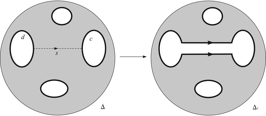
125 a) b) Figure 33: 125

126 is a word in H λ \ {1} representing an element of N λ in G. Note also that our surgery does not affect cuts of except for r. Thus the system of cuts T 1 in 1 may obtained from T as follows. Since is connected and simply connected, there is a unique sequence c = c 0, t 1, c 1,..., t l, c l = ext, where c 0,..., c l are (distinct) components of, t i T, and (up to orientation) t i connects c i 1 to c i, i = 1,..., l (Fig. 33a). We set T 1 = (T \ {r, t 1 }) {u, v}. Thus 1 D(W ) and τ( 1 ) < τ( ). Indeed 1 and have the same number of holes and l(t) l(t) 1. t T 1 t T 1 This contradicts the choice of. Finally suppose that c is connected to another component d of int, d c. To be definite, assume that c and d are labelled by words in H λ \ {1}. Again without loss of generality we may assume that there is a path s without self intersections in such that s d, s + c, Lab(s) is a word in H λ \ {1}, and s has no common points with and paths from T except for s and s +. Let us cut along s and denote by 1 the obtained diagram (Fig. 33b). This transformation does not affect ext and the only changed internal boundary component has label Lab(c)Lab(s) 1 Lab(d)Lab(s), which is a word in H λ \ {1}. This word represents an element of N λ in G as N λ H λ. We now fix an arbitrary system of cuts in 1. Then 1 D(W ) and the number of holes in 1 is smaller that the number of holes in. We get a contradiction again. 7.3 The general case The aim of this section is to prove the general version of the group theoretic Dehn filling theorem. We start by recalling the general settings. Let G be a group, {H λ } λ Λ a collection of subgroups of G, X a subset of G that generates G together with the union of H λ s. As usual, d λ denotes the corresponding distance function on H λ defined using Γ(G, X H). Given a collection N = {N λ } λ Λ of subgroups of G such that N λ H λ for all λ Λ, we define s(n) = min λ Λ min h N λ \{1} d λ (1, h). The Dehn filling of G associated to this data is the quotient group G Ḡ = G/ N λ. Let X be the natural image of X in Ḡ and let λ Λ H = λ Λ H λ /N λ. Our main result is the following result. When talking about loxodromic, parabolic, or elliptic elements of the group G or its subgroups (respectively, Ḡ) we always mean that these elements are loxodromic, parabolic, or elliptic with respect to the action on Γ(G, X H) (respectively, Γ(Ḡ, X H)). 126

127 Theorem Suppose that a group G is weakly hyperbolic relative to a collection of subgroups {H λ } λ Λ and a relative generating set X. Then there exists a constant R > 0 such that for every collection N = {N λ H λ λ Λ} satisfying the following hold. s(n) > R, (77) (a) The natural map from H λ /N λ to Ḡ is injective for every λ Λ. (b) Ḡ is weakly hyperbolic relative to H and X. (c) The natural epimorphism ε: G Ḡ is injective on X. (d) Every element of Ker(ε) is either conjugate to an element of N λ for some λ Λ or is loxodromic. Moreover, translation numbers of loxodromic elements of Ker(ε) (with respect to the action on Γ(G, X H)) are uniformly bounded away from zero. (e) Ker(ε) = λ Λ t Tλ N t λ for some subsets T λ G. (f) Every loxodromic (respectively, parabolic or elliptic) element of Ḡ is the image of a loxodromic (respectively, parabolic or elliptic) element of G. The proof of parts (a)-(c) of Theorem 7.15 repeats the proof of the main result of [119]. It consists of a sequence of lemmas, which are proved by induction on the rank of a diagram defined as follows. We assume that the reader is familiar with the terminology and notation introduced in the previous section. Let where D = D(2, 0) be the constant from Proposition R = 4D, (78) Definition Given a word W in the alphabet X H representing 1 in Ḡ, we denote by q(w ) the minimal number of holes among all diagrams from D(W ). Further we define the type of W by the formula θ(w ) = (q(w ), W ). The set of types is endowed with the natural order (as in Definition 7.13). The next three results are proved by common induction on q(w ). Recall that a word W in X H is called (λ, c) quasi geodesic (in G) for some λ 1, c 0, if some (or, equivalently, any) path in Γ(G, X H) labelled by W is (λ, c) quasi geodesic. Lemma Suppose that W is a word in the alphabet X H representing 1 in Ḡ and is a diagram of minimal type in D(W ). Then: (a) Assume that for some λ Λ, p and q are two connected H λ subpaths of the same component c of int, then there is an H λ component r of such that p and q are subpaths of κ(r). 127

128 Figure 34: (b) If W is (2, 0) quasi geodesic and q(w ) > 0, then some component of int is connected to an H λ subpath of ext for some λ Λ. (c) If W is a word in the alphabet H λ \ {1} for some λ Λ, then W represents an element of N λ in G. Proof. For q(w ) = 0 the lemma is trivial. Assume that q(w ) > 0. Let us prove the first assertion. Let x (respectively y) be an ending vertex of a certain essential edge of p (respectively q). Passing to a 0 refinement of, we may assume that x and y do not belong to any cut from the cut system T of. Applying Lemma 7.11 we get a paths s in connecting x to y such that Lab(s) is a word in the alphabet H λ \ {1} and s does not intersect any path from T. Let us denote by Ξ the subdiagram of bounded by s and the segment u = [x, y] of c ±1 such that Ξ does not contain the hole bounded by c (Fig. 34). Note that V Lab( Ξ) is a word in the alphabet H λ \ {1} and q(v ) < q(w ). By the third assertion of our lemma, V represents an element of N λ. Up to a cyclic shift, the label of the external boundary component of the subdiagram Σ = Ξ c of is a word in H λ \ {1} representing the same element as Lab(c ±1 )Lab(u) 1 V ±1 Lab(u) in G. As N λ is normal in H λ and Lab(u) represents an element of H λ in G, Lab( ext Σ) represents an element of N λ in G. If Ξ contains at least one hole, we replace Σ with a single hole bounded by ext Σ (Fig. 34). This reduces the number of holes in and we get a contradiction. Therefore Ξ is simply connected. In particular, the path u does not intersect any cut from T. This means that p and q are covered by the image of the same H λ component of. To prove the second assertion we suppose that for every component c i of int, no H λ subpath of ext is connected to c. Then Proposition 7.14 and the first assertion of our lemma imply that each component c i of int gives rise to H λ components a i1,..., a il of for some l = l(i) such that κ(a ij ) c i, j = 1,..., l, and µ(a i1 ),..., µ(a il ) are isolated H λ components of the cycle P = µ( ) in Γ(G, X H). For each component c i of int ( ), we fix a vertex o i c i such that o i = t or o i = t + for some t T and denote by g i the element represented by Lab(c i ) when we read this label 128