Convergence Order Studies for Elliptic Test Problems with COMSOL Multiphysics

Transcription

1 Convergence Order Studies for Elliptic Test Problems with COMSOL Multiphysics Shiming Yang and Matthias K. Gobbert Abstract. The convergence order of finite elements is related to the polynomial order of the basis functions used on each element, with higher order polynomials yielding better convergence orders. However, two issues can prevent this convergence order from being achieved: the poor approximation of curved boundaries by polygonal meshes and lack of regularity of the PDE solution. We show studies for Lagrange elements of degrees 1 through 5 applied to the classical test problem of the Poisson equation with Dirichlet boundary condition. We consider this problem in 1, 2, and 3 spatial dimensions and on domains with polygonal and with curved boundaries. The observed convergence orders in the norm of the error between FEM and PDE solution demonstrate that they are limited by the regularity of the solution and are degraded significantly on domains with non-polygonal boundaries. All numerical tests are carried out with COMSOL Multiphysics. Key words. Poisson equation, a priori error estimate, convergence study, mesh refinement. AMS subject classifications (2000). 35J67, 35J70, 41A25, 65M60, 68N99. 1 Introduction The finite element method (FEM) is widely used as a numerical method for the solution of partial differential equation (PDE) problems, especially for elliptic PDEs such as the Poisson equation with Dirichlet boundary conditions u = f in Ω (1.1) u = r on Ω, (1.2) where f and r denote given functions on the domain Ω and on its boundary Ω, respectively. Here, the domain Ω R d is assumed to be a bounded, open, simply connected, and convex set in d = 1, 2, 3 dimensions with piecewise smooth boundary Ω. The FEM solution u h will typically incur an error against the true solution u of the PDE (1.1) (1.2). This error can be quantified by bounding the norm of the error u u h in terms of the mesh spacing h of the finite element mesh. Such estimates have the form u u h C h q, where C is a problem-dependent constant independent of h and the constant q indicates the order of convergence of the FEM, as the mesh spacing h decreases. We see from this form of the error estimate that we need q > 0 for convergence as h 0. More realistically, we wish to have for instance q = 1 for linear convergence, q = 2 for quadratic convergence, or higher values for even faster convergence. The natural norm of the finite element method for elliptic problems is the so-called energy norm, which can be related to the norm u u h H 1 (Ω) associated with the Sobolev space H 1 (Ω) that the solution u lives in for elliptic PDEs with appropriate properties, e.g., [1, Chapter II], [3, Chapter 5]. This norm involves both the error and its (weak) derivative. Again under appropriate assumptions, it is possible to derive bounds on a norm of the error itself, not involving its derivatives. This norm u u h L 2 (Ω) is the L 2 -norm associated with the space L 2 (Ω) of square-integrable functions, that is, the space of all functions v(x) whose square Department of Mathematics and Statistics, University of Maryland, Baltimore County, 1000 Hilltop Circle, Baltimore, MD 21250, {shiming1,gobbert}@math.umbc.edu 1

2 v 2 (x) can be integrated over all x Ω without becoming infinite. The norm is defined concretely as the square root of that integral, namely ( 1/2 v L 2 (Ω) := v 2 (x) dx). (1.3) Using the L 2 -norm to measure the error of the FEM allows the computation of norms of errors also in cases where the solution and its error do not have derivatives. Thus, we use it in the following because it can quantify the expected error behavior for certain highly non-smooth problems. In the finite element method, assume that T h is a quasi-uniform mesh of the domain (including its boundary) Ω, where h denotes the mesh size of T h, e.g., defined as the maximum side length of all elements K T h. Then consider u h P p as the FEM solution using the Lagrange finite elements of degree p, which approximate the PDE solution u at several points in each element K T h such that the restriction of u h to each element K is a polynomial of degree up to p and u h is continuous across all boundaries between neighboring elements throughout Ω. For the case of linear (degree p = 1) Lagrange elements, we have the well known a priori bound, e.g., [1, Section II.7]. u u h L 2 (Ω) C h 2. (1.4) This theorem says that the convergence order is one higher than the polynomial degree used by the Lagrange elements. This result can be stated more generally when using Lagrange elements with degree p 1, such that u u h L 2 (Ω) C h p+1. (1.5) The bound in (1.4) is therefore a special case of the bound in (1.5) with p = 1. Both results stated above require a number of assumptions on the problem (1.1) and (1.2) and the finite element method used. One assumption is that the problem has a solution that is sufficiently regular, as expressed by the number of continuous derivatives that it has. In the context of the FEM, it is appropriate to consider weak derivatives. Based on these, we define the Sobolev function spaces H k (Ω) of order k of all functions on Ω that have weak derivatives up to order k that are square-integrable in the sense of the space L 2 (Ω) above. It turns out that the convergence order of the FEM with Lagrange elements with degree p is limited by the regularity order k of the PDE solution. Using the concept of weak derivative, the error bound can be stated as u u h L 2 (Ω) C h q, q = min{k, p + 1}. (1.6) This says that the convergence order of the FEM is regularity order k of the PDE solution or one higher than the polynomial degree p, whichever is smaller. This points out that higher-order Lagrange finite elements do not secure a higher convergence order of the FEM error, because two contradictory requirements are hiding there. We need higher-order regularity for the PDE solution to guarantee higher-order convergence. For instance, in order to see convergence of order q = 3 for quadratic Lagrange elements with degree p = 2, we need to have u H k (Ω) with k = 3. To obtain such regularity, we need to have a domain Ω with a smooth boundary Ω, not just a piecewise smooth boundary [1, Section II.7]. This assumption can be satisfied easily for certain domains, such as a disk in two or a ball in three dimensions. For such domains however, it is clear that an ordinary finite element mesh T h comprising of polygonal elements (such as triangles or tetrahedra) is in fact not a partition of Ω with a smooth boundary, which is another assumption of all theorems. This highlights the need for finite elements, such as isoparametric elements, that can represent a curved boundary [1, Chapter III]. In this note, we design a group of test problems to demonstrate numerically how these assumptions affect the expected convergence order. All test problems are designed to have a known true PDE solution u to allow for a direct computation of the error u u h against the FEM solution and its norm in (1.6). The convergence order q is then estimated from these computational results by the following steps: Starting from some initial mesh, we refine it uniformly repeatedly, such that the mesh spacing h of each mesh is halved. For instance in two dimensions, every triangle is sub-divided into four triangles; if the mesh spacing h is defined as the maximum side length of all triangles, this procedure halves the value of h in each refinement. Let r denotes the number of refinement levels from the initial mesh and E r := u u h L2 (Ω) the error norm 2

3 on that level. Then assuming that E r = Ch q, the error for the next coarser mesh with mesh spacing 2h is E r 1 = C(2h) q = 2 q Ch q. Their ratio is then R r = E r 1 /E r = 2 q and Q r = log 2 (R r ) provides us with a computable estimate for q in (1.6) as h 0. Notice that the technique described here uses the known true PDE solution u; this is in contrast to the technique described in [4] that worked for Lagrange elements with p = 1 without knowing the PDE solution u. In the following studies, we consider the case of a problem with a smooth solution in Section 2 and a non-smooth solution in Section 3 to demonstrate the restriction of convergence order predicted by (1.6). That is, the problem in Section 2 has a solution that has infinitely many continuous derivatives in the classical sense and thus does not pose any restriction in (1.6), rather we expect the behavior predicted by (1.5) for Lagrange elements of degree p 1. By contrast, the non-smooth problem in Section 3 is chosen to have an extremely non-smooth forcing term in the Dirac delta function δ(x), for which solutions can only be expected to satisfy u H 2 d/2 (Ω) for Ω R d, d = 1, 2, 3. Thus, the convergence order predicted by (1.6) is restricted to q = 2 d/2, d = 1, 2, 3, for Lagrange element with any degree p 1. This example indicates that for highly non-smooth problems the computational effort associated with higher-degree FEM is not likely to gain the expected improvement in accuracy and it turns out that one might want to limit the degree of Lagrange element used to p = 2. The convergence orders predicted according to these arguments are summarized in Table 1 for the smooth and non-smooth test problems with domains Ω R d in d = 1, 2, 3 dimensions. The prediction summarized in Table 1 do not account for the degradation of convergence behavior that we expect from Ω being a domain with non-polygonal boundary that cannot be meshed by T h without error. Therefore, within each case of smooth and non-smooth problems in Sections 2 and 3, we check the impact of the domain s shape: We realize that in one spatial dimension, the only possible domain shape is an interval such as ( 1, 1), and this does not suffer from any degradation at the boundary; this case is contained within the following designs of both polygonal and non-polygonal domains. In Sections 2.1 and 3.1, we consider the square ( 1, 1) 2 in two and the cube ( 1, 1) 3 in three dimensions as the simplest polygonal domain, and in Sections 2.2 and 3.2, we consider the unit disk B (2) 1 (0) in two and the unit ball B(3) 1 (0) as the simplest nonpolygonal domain, which has also the smoothest boundary possible. These studies are a generalization of the two-dimensional studies reported in [5]. Table 2 summarizes all observed convergence orders in the same form as Table 1. These results are collected from the convergence order estimates in Tables 3 through 12 in the following Sections 2 and 3. It is noted that COMSOL Multiphysics does not have Lagrange elements of degree 5 in three dimensions, as indicated by the N/A in the table. In many cases, the results in both tables agree with each other as expected. We point out again that the d = 1 domain is the same for both domain shapes, since B (1) 1 (0) = ( 1, 1) in one dimension. In the case of the non-smooth test problem in d = 1 dimension, it turns out that the true solution to the problem is a piecewise affine function and thus is represented by the FEM solution using any Lagrange element with p 1; hence, its error only consists of round-off already for the coarsest mesh considered and this optimal result is not improved upon by finer meshes, thus we report the convergence order as infinity in Table 2. For the smooth problem on the disk/ball domains in d = 2, 3 dimensions, we see some degradation of convergence order, as we had expected, with the three-dimensional case being particularly bad. Notice that the expected convergence order of the nonsmooth test problem is still smaller due to the lack of regularity of the solution, so we find this limit to still dominate even for the unit ball in d = 3 dimensions. The solutions for all test problems in these studies are implemented in COMSOL Multiphysics of version 3.3. We use techniques derived from the script file provided in [4] to compute all convergence orders, which are summarized in Table 2. The computations were performed on the machine kali, which is part of the UMBC High Performance Computing Facility ( 3

4 Table 1: Summary of the convergence order predicted by (1.6) for smooth and non-smooth test problems on square/cube domains Ω = ( 1, 1) d R d and disk/ball domains Ω = B (d) 1 (0) Rd in d = 1, 2, 3 dimensions for Lagrange elements of degree 1,..., 5. Predicted convergence order based on the true solution Ω = ( 1, 1) d R d Ω = B (d) 1 (0) Rd d = 1 d = 2 d = 3 d = 1 d = 2 d = 3 Lag Lag smooth Lag Lag Lag Lag Lag Lag Lag Lag Ω = ( 1, 1) d R d Ω = B (d) 1 (0) Rd d = 1 d = 2 d = 3 d = 1 d = 2 d = 3 Lag Lag non-smooth Lag Lag Lag Lag Lag Lag Lag Lag Table 2: Summary of the observed convergence order for smooth and non-smooth test problems on square/cube domains Ω = ( 1, 1) d R d and disk/ball domains Ω = B (d) 1 (0) Rd in d = 1, 2, 3 dimensions for Lagrange elements of degree 1,..., 5. Observed convergence order based on the true solution Ω = ( 1, 1) d R d Ω = B (d) 1 (0) Rd d = 1 d = 2 d = 3 d = 1 d = 2 d = 3 Lag Lag smooth Lag Lag Lag Lag Lag Lag Lag5 6 6 N/A Lag N/A Ω = ( 1, 1) d R d Ω = B (d) 1 (0) Rd d = 1 d = 2 d = 3 d = 1 d = 2 d = 3 Lag Lag non-smooth Lag Lag Lag Lag Lag Lag Lag5 1 N/A Lag5 1 N/A 4

5 2 Smooth Test Problems In this section, we test smooth problems in domains both square and disk in dimensions from 1 to 3. For the test problem, the right-hand side of Poisson equation f(x) in (1.1) and its boundary condition r(x) in (1.2) are detailed in the following. The right-hand side function is f(x) = π 4 π 2 π 2 πx ( cos 2 ) for d = 1, 1 πρ ρ sin 2 + π πρ 2 cos 2 ( ) for d = 2, 2 πρ ρ sin 2 + π πρ 2 cos 2 for d = 3, where ρ = x 2 + y 2 in 2-D, and ρ = x 2 + y 2 + z 2 in 3-D. This function satisfies the standard assumption of f L 2 (Ω) using in classical FEM theory. The problems are chosen such that we know the true solution u true (x). Using this fact, the Dirichlet boundary condition function r is indeed chosen equal to the true solution, thus the equation r(x) = u true (x) = cos πx 2 for d = 1, cos π x 2 +y 2 2 for d = 2, cos π x 2 +y 2 +z 2 2 for d = 3. lists both functions. We use these functions on all domains in this section, where we notice that on the disk/ball domains B (d) 1 (0), the boundary condition becomes a homogeneous Dirichlet condition r = 0 by construction of the true solution. Figures 1 and 2 illustrate the solution and the extremely coarse mesh used to compute it in the case of two and three dimensions, respectively. The default quadratic Lagrange elements are used in these plots. The true PDE solutions u true (x) in (2.2) are infinitely often differentiable in the classical sense, and hence the regularity order k does not limit the predicted convergence order q = min{k, p + 1} for any degree p of the Lagrange elements. The Tables 3 through 5 summarize the results for the smooth test problem. A coarse initial mesh for Ω is created in each case, then several successive refinements are made. The tables list the number of mesh elements N e, number of points (vertices) in the mesh N p, and the number of degrees of freedom (DOF) as used by COMSOL. The following column list the norm of the observed true error between FEM solution and the true PDE solution with the convergence order q (est ) estimated as Q r, described in the Introduction. The final column lists the results of an analogous procedure based on using the numerical solution on the finest mesh as reference solution in place of the true solution, detailed in [4] for Lagrange elements of degree 1, to estimate the error without using the true PDE solution; this technique can be generalized to Lagrange elements of degree Square Domain Cases For the smooth test problems, the domain is selected as square in all dimensions, namely, Ω = ( 1, 1) R d, d = 1, 2, 3, which can be decomposed by polygonal elements without error. Tables 3, 4, and 5 summarize the results for these cases. In these tables, we observe that the convergence order estimate q est = Q r is consistent with the predicted value q = p + 1 for all p = 1,..., 5. Hence, it is worth of adopting higher degree of Lagrange elements to obtain higher convergence orders under current settings. 2.2 Disk Domain Cases We consider the same f and r in (1.1) and (1.2) for the PDE as in Section 2.1. The only difference from above cases for the smooth test problems is that the domain is selected as disk in all dimensions, namely Ω = B (d) 1 (0) Rd, d = 1, 2, 3. We notice that the Dirichlet boundary condition is in fact homogeneous r 0 in this case. In two and three dimensions, these domains have curved boundaries. Recall that the one-dimensional domain is identical with the one in the previous subsection, hence Tables 3, 6, and 7 summarize the results for these domains. In two dimensions, from Table 7(a) to Table 5 (2.1) (2.2)

6 7(b), we can observe the fact that the order of convergence order are still nominal q = p + 1. However, from Table 7(c) to Table 7(e), we see a slight degradation for p = 3, and no improvement for convergence order in the case of over p = 3, though we notice that the absolute errors still decrease. In three dimensions, numerical results are listed from Table 8(a) to Table 8(d) for the elements available in COMSOL. In the unit ball case, as the degree of Lagrange element increases, the convergence order approaches to 0, which means that in such case polynomials of higher degrees do not improve the convergence order as significantly. This can be interpreted in as the domination of quadrature error over the finite element error in high dimension and with higher degree of Lagrange element polynomials. Notice however that the observed errors themselves still get somewhat smaller for larger degrees of Lagrange elements, so their use is still somewhat justified. We point out that the use of a homogeneous Dirichlet boundary condition likely minimized the error incurred by the quadrature near the curved boundary, so we suspect that results could be worse. 3 Non-smooth Test Problems For non-smooth test problems, we choose domain shapes the same as smooth cases, such that Ω = ( 1, 1) d, and Ω = B (d) 1 (0) Rd, d = 1, 2, 3. The source term f for different dimensions are set as the Dirac delta function f(x) = δ(x). The Dirac delta function models a point source and is mathematically defined by requiring δ(x ˆx) = 0 for all x ˆx while simultaneously ϕ(x)δ(x ˆx)dx = ϕ(ˆx) for any continuous function ϕ(x). Based on the weak formulation of the problem, the finite element method is able to deal with this function. That is, the PDE is integrated with respect to a smooth test function ϕ(x) so that the right-hand side becomes ϕ(x)δ(x)dx = ϕ(0). If the point 0 is chosen as a mesh point of the FEM mesh, Ω then the test function evaluated at 0 in turn will equal 1 for the FEM basis function centered at this mesh point and 0 for all others. As explained in the COMSOL manual, a point source modeled by the Dirac delta distribution can be implemented in COMSOL by adding the test function u_test at that mesh point to the weak term. We then consider (1.1) (1.2) with f(x) = δ(x) and r = u true (x) with 1 x 2 for d = 1, ln x u true (x) = 2 +y 2 2π for d = 2, (3.1) 1 for d = 3 8π x 2 +y 2 +z 2 As before, r = 0 on the boundary of B (d) 1 (0) by construction. Figures 3 and 4 illustrate the solution and the extremely coarse mesh used to compute it in the case of two and three dimensions, respectively. The default quadratic Lagrange elements are used in these plots. Notice that the true solutions have a singularity at the origin 0, where they tend to infinity. Thus, the solutions are not differentiable everywhere in Ω and thus not in any space of continuous or continuously differentiable functions. However, recall the Sobolev Embedding Theorem [6, Section 9.3]. Since v(x)δ(x)dx = v(0) for any continuous function v(0), and the Sobolev space H d/2+ε is continuously embedded in the space of continuous function C 0 (Ω) in d = 1, 2, 3 dimensions for any ε > 0, one can argue that δ is in the dual space of v H d/2+ε (Ω), that is, δ H d/2 ε (Ω). Since the solution u of this second-order elliptic PDE is two orders smoother, we obtain the regularity u H 2 d/2 ε (Ω) or k 2 d/2 in (1.6), which suggests that higher-order Lagrange elements do not provide any significantly better results. 3.1 Square Domain Cases In [2, Chapter 4], steps are illustrated for implementing the Dirac delta function as source term. Similar steps in smooth cases are repeated, which produce tables describing the convergence order for non-smooth cases with different degrees of Lagrange elements. Table 8 lists the results for non-smooth test problem in 1-D. It can be observed that the increasing of degree of Lagrange element does not improve convergence order significantly. As we see, the convergence orders do not represent any regularity. However, we see that the actual errors are on the order of to and in fact increase with polynomial order and with mesh refinement. This is explained by the fact that the solution in 1-D is piecewise linear and already approximated with only round-off error by linear Lagrange elements on the coarsest mesh. In light of this, 6

7 we report the convergence orders in Table 2 as infinity, which is better than and does not contradict the expected convergence order of q = 2 d/2 = 1.5 for d = 1. In fact, higher-order elements or a finer mesh only lead to accumulating more round-off error in the calculations, which is why the error increases in the later results in the table. Data in Table 9 show that the higher degree of Lagrange element does not increase the convergence order, where q = 1 for almost every refine level and all 5 kinds of Lagrange elements. Taking Table 10 into consideration, we can find that convergence orders approach to 0.5. All of these agree with the prediction that q = 2 d/2 for non-smooth problems in d = 1, 2, 3 dimensions. 3.2 Disk Domain Cases In another case for non-smooth problem, we choose the domain shapes to be disk, such that Ω = B (d) 1 (0) R d, d = 1, 2, 3. By repeating all test cases in dimension d = 1, 2, 3, and 5 types of Lagrange elements, we collect Tables 11 and 12 describing the convergence order for the non-smooth cases with different degrees of Lagrange elements in two and three dimensions, respectively. By the limitation of regularity of PDE solution, we see that domain shapes have changed, however, the error convergence orders behave similarly to the square s. That is, the degrading associated with the curved boundary of B (d) 1 (0) is already dominated by the restriction given by the regularity order k = 2 d/2 for this highly non-smooth problem. 4 Conclusions In this report, the test problems are Poisson equation with smooth or non-smooth solutions. The domains are chosen as open square or disk in all dimension d, d = 1, 2, 3, which possess polygonal and curved boundaries, respectively. With true solution available, we can calculate errors with the FEM solution against the true solution. Piecewise polynomials, linear, quadratic, cubic, quartic and quintic, are used to approximate functions. From the observed data, it is confirmed that the regularity of solution and the shape of domains affect the convergence order. On one hand, higher order polynomials of Lagrange element give better convergence orders for smooth problem on polygonal domains, which are worth of use. For example, quadratic and cubic Lagrange elements provide higher order of convergence order than linear Lagrange elements do, and the computing expense does not compensate such benefit. On the other hand, it is noticed that higher degree of Lagrange elements do not behave as expected in domain that has curved boundary, e.g., the disk and ball. Especially in 2-D and 3-D cases, the convergence orders are damaged and not competitive with those on the polygonal domains. We explain this by error that is introduced by the inexact approximation of curved boundary with polynomial triangulation. Moreover, the convergence order is also limited due to the PDE solution lacking of regularity. In non-smooth test problems, test results agree with the theoretical expectation that convergence order is 2 d/2 in d = 1, 2, 3 dimensions. In future studies, we are interested in being able to observe the error and its convergence order without knowing the true PDE solution. One technique to do this is to replace the true solution by a reference solution taken from the solution on the finest mesh. The tables in this note show these results in the final column for those Lagrange elements for which we could compute it, implementing ideas from [4] for linear Lagrange elements and extending them to quadratic elements, where possible. In those cases, the observations by the reference error track those of the true error very well, thus confirming the validity of the approach. Future work has to extend this idea to higher-order Lagrange elements. 7

8 References [1] Dietrich Braess, Finite Elements: Theory, fast solvers, and applications in solid mechanics, Cambridge University Press, third edition, [2] COMSOL Multiphysics: Users Guide, version 3.3, COMSOL AB., 2006 [3] Mark S. Gockenbach, Understanding and Implementting the Finite Element Method, SIAM, [4] Matthias K. Gobbert. A Technique for the Quantitative Assessment of the Solution Quality on Particular Finite Elements in COMSOL Multiphysics. In: Vineet Dravid, editor, Proceedings of the COMSOL Conference 2007, Boston, MA, pp , [5] Matthias K. Gobbert and Shiming Yang. Numerical Demonstration of Finite Element Convergence for Lagrange Elements in COMSOL Multiphysics. In: Vineet Dravid, editor, Proceedings of the COMSOL Conference 2008, Boston, MA, in press, [6] Leszek Demkowicz. Computing with H p -adaptive Finite Elements: Volume 1: One and Two Dimensional Elliptic and Maxwell Problems. CRC Press,

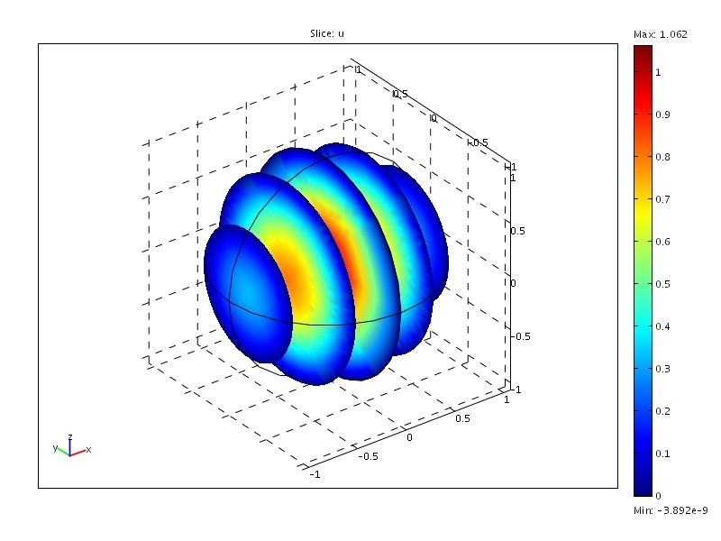
9 Figure 1: Mesh and solution plot for 2D polygonal (left) and non-polygonal (right) domains, smooth case. Figure 2: Mesh and solution plot for 3D polygonal (left) and non-polygonal (right) domains, smooth case. 9

10 Table 3: Convergence study for the smooth test problem on Ω = ( 1, 1) e e e-002 (1.9811) e-002 (1.9791) e-003 (1.9953) e-003 (1.9808) e-004 (1.9988) e-004 (2.0409) e-004 (1.9997) N/A (a) Lag e e e-004 (2.9898) e-004 (2.9540) e-005 (2.9974) e-005 (2.9559) e-006 (2.9994) e-006 (2.9135) e-007 (2.9998) N/A (b) Lag e-004 N/A e-005 (3.9916) N/A e-007 (3.9979) N/A e-008 (3.9995) N/A e-009 (3.9999) N/A (c) Lag e-006 N/A e-008 (4.9947) N/A e-009 (4.9987) N/A e-011 (4.9996) N/A e-012 (4.9270) N/A (d) Lag e-007 N/A e-009 (5.9945) N/A e-011 (6.0066) N/A e-013 (5.4684) N/A e-012 ( ) N/A (e) Lag5 10

11 Table 4: Convergence study for the smooth test problem on Ω = ( 1, 1) e e e-002 (1.8619) e-002 (1.8882) e-002 (1.9461) e-002 (1.9843) e-003 (1.9818) e-003 (2.1975) e-003 (1.9941) N/A (a) Lag e e e-003 (3.2373) e-003 (3.1767) e-004 (3.0558) e-004 (3.0433) e-005 (2.9980) e-005 (2.9958) e-006 (2.9912) N/A (b) Lag e-003 N/A e-004 (3.9880) N/A e-006 (3.9983) N/A e-007 (4.0017) N/A e-008 (4.0014) N/A (c) Lag e-005 N/A e-006 (5.3369) N/A e-008 (5.2172) N/A e-009 (5.1163) N/A e-011 (5.0605) N/A (d) Lag e-005 N/A e-007 (5.9258) N/A e-009 (5.9756) N/A e-011 (6.0004) N/A e-013 (5.4916) N/A (e) Lag5 11

12 Table 5: Convergence study for the smooth test problem on Ω = ( 1, 1) e e e-001 (1.5549) e-001 (1.5655) e-002 (1.9283) e-002 (1.9798) e-002 (1.9848) e-002 (2.2222) e-003 (2.0007) N/A (a) Lag e e e-002 (3.4627) e-002 (3.6256) e-003 (2.9325) e-003 (2.9626) e-004 (2.9583) e-004 (3.1025) e-005 (2.9682) N/A (b) Lag e-002 N/A e-003 (3.7043) N/A e-005 (4.0209) N/A e-006 (4.0329) N/A (c) Lag e-003 N/A e-005 (5.3585) N/A e-006 (4.9856) N/A e-008 (5.0149) N/A (d) Lag4 12

13 Table 6: Convergence study for the smooth test problem on Ω = B (2) 1 (0) R e e e-003 (1.9652) e-003 (1.9670) e-003 (1.9878) e-003 (2.0098) e-004 (1.9961) e-004 (2.1597) e-004 (1.9988) N/A (a) Lag e e e-005 (2.9238) e-005 (2.9454) e-006 (2.9769) e-006 (2.9933) e-006 (2.9888) e-007 (3.0135) e-007 (2.9941) N/A (b) Lag e-005 N/A e-006 (3.8904) N/A e-007 (3.8234) N/A e-008 (3.7384) N/A e-009 (3.6562) N/A (c) Lag e-006 N/A e-007 (3.6185) N/A e-008 (3.5128) N/A e-009 (3.4903) N/A e-010 (3.4908) N/A (d) Lag e-006 N/A e-007 (3.9648) N/A e-008 (3.6557) N/A e-009 (3.5222) N/A e-010 (3.4936) N/A (e) Lag5 13

14 Table 7: Convergence study for the smooth test problem on Ω = B (3) 1 (0) R e-001 NaN e-002 (1.7661) e-002 ( NaN) e-002 (1.8762) e-002 (1.9775) e-003 (1.8859) e-003 (2.1687) e-003 (1.6515) N/A (a) Lag e-002 N/A e-003 (2.1279) N/A e-003 (1.4683) N/A e-003 (0.2692) N/A e-003 (0.1742) N/A (b) Lag e-003 N/A e-003 (1.5764) N/A e-004 (0.4826) N/A e-004 (0.0454) N/A (c) Lag e-003 N/A e-004 (1.1077) N/A e-004 (0.3317) N/A e-004 (0.1302) N/A (d) Lag4 14

15 Figure 3: Mesh and solution for 2D polygonal (left) and non-polygonal (right) domains, non-smooth case. Figure 4: Mesh and solution plot for 3D polygonal (left) and non-polygonal (right) domains, non-smooth case. 15

16 Table 8: Convergence study for the non-smooth test problem on Ω = ( 1, 1) e e e-016 ( -Inf) e-015 ( ) e-017 (1.0441) e-015 (0.0354) e-015 ( ) e-015 (0.4345) e-015 ( ) N/A (a) Lag e e e-015 ( ) e-013 (0.0172) e-015 ( ) e-013 (0.0873) e-014 ( ) e-014 (0.4169) e-013 ( ) N/A (b) Lag e-015 N/A e-015 ( ) N/A e-014 ( ) N/A e-014 ( ) N/A e-013 ( ) N/A (c) Lag e-015 N/A e-014 ( ) N/A e-014 ( ) N/A e-013 ( ) N/A e-013 ( ) N/A (d) Lag e-015 N/A e-014 ( ) N/A e-013 ( ) N/A e-013 ( ) N/A e-012 ( ) N/A (e) Lag5 16

17 Table 9: Convergence study for the non-smooth test problem on Ω = ( 1, 1) e e e-002 (0.8950) e-002 (0.9467) e-002 (0.9747) e-003 (1.0007) e-003 (0.9925) e-003 (1.0188) e-003 (0.9979) N/A (a) Lag e e e-003 (0.9910) e-003 (0.9340) e-003 (0.9996) e-003 (0.8969) e-003 (1.0000) e-003 (0.9620) e-004 (1.0000) N/A (b) Lag e-003 N/A e-003 (0.9936) N/A e-003 (0.9997) N/A e-004 (1.0000) N/A e-004 (1.0000) N/A (c) Lag e-003 N/A e-003 (0.9996) N/A e-003 (1.0000) N/A e-004 (1.0000) N/A e-004 (1.0000) N/A (d) Lag e-003 N/A e-003 (1.0001) N/A e-003 (1.0000) N/A e-004 (1.0000) N/A e-004 (1.0000) N/A (e) Lag5 17

18 Table 10: Convergence study for the non-smooth test problem on Ω = ( 1, 1) e e e-002 (0.5530) e-002 (0.7210) e-002 (0.5297) e-002 (0.7123) e-002 (0.5057) e-002 (0.6455) e-002 (0.5009) N/A (a) Lag e e e-002 (0.5323) e-002 (0.5293) e-002 (0.5095) e-002 (0.5799) e-002 (0.5002) e-002 (0.9926) e-003 (0.5000) N/A (b) Lag e-002 N/A e-002 (0.5004) N/A e-002 (0.5001) N/A e-003 (0.5000) N/A (c) Lag e-002 N/A e-003 (0.5084) N/A e-003 (0.5001) N/A e-003 (0.5000) N/A (d) Lag4 18

19 Table 11: Convergence study for the non-smooth test problem on Ω = B (2) 1 (0) R e e e-003 (1.0227) e-003 (0.7650) e-003 (1.0104) e-003 (0.7103) e-003 (1.0040) e-003 (0.8790) e-003 (1.0013) N/A (a) Lag e e e-003 (1.0018) e-003 (0.8107) e-003 (0.9993) e-003 (0.8259) e-003 (1.0000) e-003 (1.0113) e-004 (1.0000) N/A (b) Lag e-003 N/A e-003 (1.0005) N/A e-003 (1.0000) N/A e-003 (1.0000) N/A e-004 (1.0000) N/A (c) Lag e-003 N/A e-003 (1.0012) N/A e-004 (1.0000) N/A e-004 (1.0000) N/A e-004 (1.0000) N/A (d) Lag e-003 N/A e-003 (1.0004) N/A e-003 (1.0000) N/A e-004 (1.0000) N/A e-004 (1.0000) N/A (e) Lag5 19

20 Table 12: Convergence study for the non-smooth test problem on Ω = B (3) 1 (0) R e-002 NaN e-002 (0.5078) e-002 ( NaN) e-002 (0.5118) e-002 (0.3836) e-002 (0.5022) e-002 (0.6093) e-002 (0.5002) N/A (a) Lag e-002 N/A e-002 (0.6779) N/A e-002 (0.4998) N/A e-002 (0.5001) N/A e-003 (0.5000) N/A (b) Lag e-002 N/A e-002 (0.4767) N/A e-002 (0.5000) N/A e-002 (0.5000) N/A (c) Lag e-002 N/A e-002 (0.6237) N/A e-002 (0.4999) N/A e-002 (0.5000) N/A (d) Lag4 20