Saturated Absorption for a Magneto-Optical Atom Trap as a Step toward Atomic Dipole Traps in a Diffraction Pattern from a Circular Aperture

Transcription

1 Saturated Absorption for a Magneto-Optical Atom Trap as a Step toward Atomic Dipole Traps in a Diffraction Pattern from a Circular Aperture A Senior Project presented to the Faculty of the Katharina Gillen California Polytechnic State University, San Luis Obispo In Partial Fulfillment of the Requirements for the Degree Bachelor of Science in Physics by Andrew Ferdinand June, Andrew Ferdinand

2 TABLE OF CONTENTS Chapter 1: Introduction Introduction. 1 Chapter 2: Theoretical Background Quantum Computing... Hyperfine Structure of Rb... Atomic Dipole Traps... Magneto-Optical Atom Trap... Saturated Absorption Chapter 3: Experiment Overview Procedure Alignment Instrumentation and Settings. Troubleshooting. Results Chapter 4: Conclusion Conclusions.. References i

3 Tables: List of Tables and Figures Table 1: Quantum Computing Approaches with the corresponding qubit systems and entanglement interactions..... Table 2: Control Panel input and analog channel Figures: Figure 1: (a) Energy structure of Rb (b) Fine structure of Rb (c) Hyperfine structure of 87 Rb [22].. Figure 2: (a) z component of the Poynting vector (closely related to the intensity of the light field) of 780-nm light incident upon a 25µm aperture. The intensity is normalized to the intensity incident upon the aperture (b) Graph of the z component of the normalized Poynting vector along the z axis [modified from 5]... Figure 3: (a) Diagram of setup (b) Relative intensity of the light field as two traps are brought together (c) Red detuned light potential-energy profile in the y direction at z=67 µm of F=1 m F =1 (solid line) and F=1 m F =-1 (dotted line) (d) Blue detuned light potential-energy profile in the y direction at z=100 µm of F=1 m F =1 (solid line) and F=1 m F =-1 [modified from 6]... Figure 4: (a) Diagram of setup (b) Relative light intensity of diffraction pattern (c)-(j) Potential energy of (b) with red detuned light for the magnetic substates of F=1 and F=2 hyperfine states [6].. Figure 5: Projection schematic. The lens focal point lies in the diffraction pattern [modified from 8]... Figure 6: (a) Picture and (b) Schematic of primary MOT components Figure 7: (a) Detuning from F=2 F =3 transition of the 2 S 1/2 2 P 3/2 manifold (b) Optical Doppler shift of photon energies of atoms with different velocities... Figure 8: (a) MOT schematic, polarity of electromagnetic coils, and magnetic field B (b) Linear dependence of magnetic field B.. Figure 9: Zeeman splitting and trapping mechanism of the MOT. Figure 10: Trap and Pump Laser transitions [22] ii

4 Figure 11: Doppler Peak in absorption spectrum around transition frequency f 0... Figure 12: Saturated absorption schematic Figure 13: Laser Schematic [modified from 22] Figure 14: Saturated Absorption Schematic... Figure 15: (a) Changing of position of beam on D by adjusting C (b) Changing direction of beam by adjusting D Figure 16: Saturated Absorption Curve τ=100ms.. Figure 17: Saturated Absorption Curves with integration times (a) τ=30ms (b) τ=100ms and (c) τ=300ms... Figure 18: Saturated Absorption Curves P=60s, τ=100ms Figure 19: Saturated absorption curves with τ=100ms and ramp periods (a) P=60s and (b) P=30s iii

5 Chapter 1: Introduction In the last quarter of the 20 th century, the merging of information science with quantum mechanics gave rise to the field of quantum information science (QIS) [1] and attracted an interdisciplinary community of physicists. Quantum information science encompasses a variety of related subtopics including quantum computing, quantum communication, and quantum algorithms. In addition to garnering the innate interest of physicists due to its applications of the fundamentals of quantum mechanics, quantum computing has been shown to have great potential to increase computing power relative to classical computers for certain types of computations. The most well-known application of quantum logic demonstrating an advantage of quantum computing is Shor s algorithm, which allows the factorization of large numbers into their prime factors exponentially faster than classical computers [2]. This specifically has captured the interest of many people because RSA encryption, the most common form of data encryption used today, relies on the difficulty of factoring large numbers to secure information. Interestingly, one of the primary benefits of quantum communication is quantum cryptography, which may lead to completely secure transmission of encryption keys [3]. The power of a quantum computer lies in its use of quantum mechanics for information processing. In a classical computer, each bit carries one piece of information and can be in the logical 1 or 0 state. Each bit in a quantum computer, called a qubit, also has a 1 and 0 each associated with a different quantum state of the system. Due to quantum mechanics, each qubit can be in a superposition of both the 1 and 0 states. Qubits can also interact with each other in ways governed by quantum mechanics not possible with classical bits, called entanglement [4]. Using these properties, quantum computers are able to perform in ways classical computers are not which, as previously mentioned, can lead to an exponential increase in computing speed. The experiment presented in this paper is in the field of neutral atom quantum computing. Neutral atom quantum computing uses the electronic states or the motional states of a neutral atom as a qubit. The goal of this experiment is to trap 87 Rb in an optical dipole trap in the diffraction pattern behind a circular aperture. When laser light is incident on a circular aperture with a radius larger than the wavelength of the light, a diffraction pattern containing localized bright and dark spots forms immediately behind the aperture. Rb atoms can be trapped in the bright or dark spots in the diffraction pattern by detuning the frequency of the laser light just slightly off resonance from a specific electronic transition [5]. Our method of trapping 87 Rb addresses the remaining obstacle in neutral atom quantum computing, the scalability of individually addressable qubits. The atomic dipole traps may also prove to be beneficial for creating a quantum computer because the position of a qubit (rubidium atom) can be controlled with the angle of incidence of the trapping laser beam on the aperture and two qubits can be brought together and apart using the polarization dependence of the energy of the traps [6]. In order to load the 87 Rb into the atomic dipole traps, we will first cool and trap the atoms in a magneto-optical atom trap (MOT). The MOT uses laser cooling to first cool a sample of Rb in a vacuum chamber. Two electromagnets on the outside of the chamber create a magnetic field which increases linearly from zero at the center of the trap, inducing position dependent Zeeman splitting of the energy levels of the rubidium atoms. Exploiting the Zeeman splitting, momentum conservation, electron transition selection rules, and through a clever use of light polarization, any atom that strays from the center of the field will be pushed back toward the center. A 1

6 localized cloud of cold 87 Rb will result in the chamber at the center of the coils. One crucial aspect of the MOT that will be addressed in this paper is the saturated absorption apparatus, which serves as part of the apparatus to detune the laser light to the correct frequency for trapping. Once we have atoms trapped in the MOT, we plan on projecting the diffraction pattern from the circular aperture onto the cloud of cold rubidium atoms [7], allowing us to transfer the rubidium atoms into the dipole traps. This paper will continue in Chapter 2 by first discussing the theoretical background of our experiment. Chapter 2 starts with a discussion of basic ideas and motivation for quantum computing along with details into neutral atom quantum computing. It continues with sections discussing the hyperfine structure of Rb, our atomic dipole traps, the cooling and trapping mechanisms of the MOT, and finishes with the theory of saturated absorption. Chapter 3 is an experimental section addressing our saturated absorption apparatus and how it works. The first section of the chapter is an overview of the apparatus and its components. The next section is on our procedure, which sets guidelines for the alignment of the saturated absorption laser beams and discusses the operation of instrumentation when performing saturated absorption scans. The final section concludes with our results and examples of successful saturated absorption scans. Chapter 4 is the conclusion, summarizing our research. Chapter 2: Theoretical Background Quantum Computing: The properties of qubits lie at the center of the power of quantum computing (QC). A qubit is a system of two quantum mechanical states analogous to a classical digital bit. Each of the two states of the qubit is considered the logical equivalent of the Boolean 1 or 0, denoted in bra-ket notation as 1 and 0 indicating they are quantum mechanical states. The power of quantum computing lies in the fact that these two states are governed by quantum mechanics, giving rise to unique logical properties and computational power. These properties allow for logical gates that are not possible with classical computers and in turn processing speed exponentially faster than classical computers for some calculations. The quantum mechanical nature of a qubits allow it to be in a linear superposition if its two basis states, 1 and 0. If a complete measurement is performed, the wavefunction of the qubit will collapse to either the 1 or 0 state. The state, or wavefuntion, of a qubit can be written as Ψ q = a 1 +b 0 where a and b are complex numbers and a 2 + b 2 =1. The coefficients a and b are related to the probability of a the qubit wavefunction collapsing into the 1 and 0 states, respectively. The expression a 2 + b 2 =1 indicates a qubit should have a 100% probability of the system being in either the 1 or 0 state. The complete state of the computer is a combination of all of the states of the qubits, for example and Similarly to the state of a single qubit, the state of the quantum computer is a linear superposition of the individual states and can be expressed as =Σ c x with Σ c x 2 =1 (1) Each coeffient c x of the complete state Ψ also is a complex number [4]. Quantum mechanics indicates that the computer can be in all possible basis states at once with the coefficient c x dictating the probability the computer will be in state if measured. Interesting and powerful 2

7 properties arise from this. One is that a quantum computer of n qubits can contain 2 n states simultaneously, as compared to the single determined state of a classical computer [4]. A powerful feature of this is the interference of intermediate states during a calculation. When an operation is being performed, the complex nature of the coefficients allows intermediate states of the quantum computer to constructively and destructively interfere, which leads to parallel computation. Exploiting parallel computation is the property which provides Shor s algorithm the power for computation times exponentially faster than classical computers [8]. A commonly known barrier to the progress of electronic technological development is the end to Moore s law. Moore s law is a prediction Gordon Moore made in 1965 which predicted the density of electronic components on an integrated circuit would double every year [9]. We have seen this prediction come true, but we are at a point where the end of the phenomenon looks to be in sight [10]. Continual development of the methods of miniaturization of electrical components along with the precision manufacturing of integrated circuits will lead to a realm where the electronic components in an integrated circuit become so small and close together, quantum interaction will impair their function. With the continuation of electronic technological development, quantum computing may some day become integrated into or take over classical systems for scientific, military, commercial, and possibly personal use. Quantum computing is an interesting field logistically because of the difference in status of the theoretical development in contrast to the experimental demonstration of quantum computation. Whereas QIS theoretical progress continually pushes the theoretical capabilities of QC, the extreme sensitivity and precision needed to experimentally create and control qubits in the fashion needed for QC makes the task of constructing a system suitable for a quantum computer an immense task. A special issue of the journal Fortschritte der Physik published in 2000 summarized many of the approaches toward creating a quantum computer and reported on the progress the approaches had made. In this issue, David DiVincenzo proposed what has become known as the DiVincenzo criteria, which are five requirements a system must have to be suitable for a physical quantum computer [11]. These requirements are frequently referenced in the QC community as a measure of viability of a system for QC. The DiVincenzo criteria are: 1. Scalable system of qubits: greater than Ability to initialize system: bring all qubits to known initial state 3. Ability to form a universal set of quantum gates: single and two qubit gates 4. Long coherence time: relative to time to enact a quantum gate, allowing ~10 6 operations before decoherence 5. Ability to read out qubit state Each of the approaches toward creating a quantum computer uses a different quantum system for its qubits. Each approach has benefits and difficulties in creating the quantum computer but, although several are close, no single approach has successfully demonstrated all the DiVincenzo criteria simultaneously. A summary of some of the approaches and the quantum systems used for qubits can be found in the table below. 3

8 Quantum Computing Approach Nuclear Magnetic Resonance (NMR) Qubit System Nuclear spin in a molecule (liquid state) or solid state Entanglement Interaction Spin-spin coupling Trapped Ions Internal spin states of trapped ions Phonons, photons, head ions Neutral Atoms in Optical Lattices Cavity Quantum Electrodynamics Internal or motional states of neutral atoms Internal or motional states of atoms in cavities, photons in cavities Electric or magnetic dipoledipole interaction, cold collisions Atom-photon interaction Optical Polarization modes of photons Prior entanglement through parametric down conversion Solid State Spin or charge in quantum dots, P impurities in Si Heisenberg exchange interaction Superconducting Charge, flux, or energy levels in a superconducting circuit using a Josephson junction NMR interaction Table 1: Quantum Computing Approaches with the corresponding qubit systems and entanglement interactions [12] The neutral atom QC community has made much progress towards creating a system of qubits which addresses all the DiVincenzo criteria, but no group has shown a system passing all the criteria. One of the prevailing techniques of creating a quantum memory with neutral atom qubits is in a three-dimensional (3D) optical lattice with some groups investigating twodimensional (2D) optical arrays of atom traps [1,13,14]. The use of counter-propagating laser beams to create standing waves in 3 dimensions leads to an interference pattern analogous to a periodic crystal lattice. Neutral atoms can be trapped in either the nodes or antinodes of the interference pattern, depending on the choice of laser light frequency. This method has promise to create a scalable system of qubits, addressing DiVincenzo criterion 1, with the downside of lack of individual addressability of the qubits [15]. Two dimensional arrays of atom traps have the benefit of much greater individual addressability of the qubits, but inherently have less ease of scalability than 3D optical lattices. A benefit of neutral atom quantum computing is the substantial previous study of atomic spectroscopy and methods of atomic-optical interaction, resulting in well established laser cooling and spectroscopic techniques [1], allowing qubit 4

9 initialization and readout (DiVincenzo criteria 2 and 5) to be performed with laser pulses. Neutral atoms interact relatively weakly with each other and with the environment, allowing for long coherence times (related to DiVincenzo criterion 4). Although it allows for relatively long coherence times, the weak coupling between neutral atoms adds difficulty in the creation of two qubit gates because of the difficulty in creating a controlled interaction between qubits. Several methods of inducing interactions between qubits have been implemented or are currently under investigation in order to entangle the qubits and demonstrate two qubit gates [1, 16, 17, 18]. The combination of single qubit gates with certain two qubit gates is sufficient for a universal set of quantum gates [19] (DiVincenzo criterion 3), meaning that any quantum algorithm can be decomposed into a combination of single qubit gates and the two qubit gate. One of the methods of inducing interaction between neutral atoms that together with single-qubit operators has demonstrated a two qubit CNOT gate is the Rydberg blockade. The CNOT gate is a two qubit gate which can comprise a universal set of quantum gates when in combination with single qubit gates [18]. A Rydberg atom is a highly excited atom which may contain a valence electron excited to a state with a principal quantum number on the order of n~100. The excited electron causes the atom to have a large electric dipole moment. The Rydberg blockade uses the interaction of the large dipole moment with the surrounding atoms to cause entanglement and create quantum gates [20]. Neutral atom quantum computing is a promising avenue in the realization of a quantum computer. The goal of our experiment is to use the localized bright or dark spots in the diffraction pattern formed immediately behind a circular aperture by detuned laser light as atomic dipole traps. The dipole traps have several characteristics beneficial for use as atom traps for qubit sites, addressing the remaining obstacle in neutral atom quantum computing, the scalability (DiVincenzo criterion 1) of individually addressable qubits. A scalable twodimensional (2D) array of individually addressable qubit sites can be created simply by allowing the laser beam to be incident on a 2D array of circular apertures. Additionally, the position of the qubits can be controlled with the angle of incidence of the laser beam on the circular apertures. By controlling the position of the qubits and exploiting the polarization dependence of the potential energy of the dipole traps, some methods of entanglement may be easier to perform by bringing pairs of qubits together and apart. Hyperfine Structure of Rb: Rubidium is an alkali metal, meaning it lies in Group I of the periodic table and has a hydrogen like electronic structure. All of the electron shells in Rb are completely filled through the n=4 shell, and the 5S shell contains a single valence electron when the atom is in its ground state. Hydrogen like atoms are relatively well understood and can be controlled and manipulated with well-established experimental techniques, such as the cooling and trapping of rubidium with a MOT as described in this paper. The hyperfine structure of an atom arises from the interactions of the three strongest magnetic moments within the atom. These interactions, or coupling, lead to the splitting of the electronic energy levels of the atom, the properties of which can be exploited for trapping an atom as well as used for the logical states of a qubit. In classical electromagnetism, moving charge creates a magnetic field. Similarly, magnetic moments in an atom can be associated with the orbital angular momentum L and the intrinsic spin angular momentum S of an atomic electron. The magnetic moments are anti-parallel in 5

10 direction and proportional in magnitude to the angular momentum vectors. The interaction of the magnetic moments causes the energy of the electron to be dependent of the alignment on L and S. The resultant electronic energy levels of an atom are proportional to the magnitude of the total electron angular momentum vector J=L+S. Incorporating the total electron angular momentum quantum number j into an analysis of an electron s energy gives rise to the fine structure of an atom. The value of j is limited by the allowed orientations of the spin and orbital angular momentum vectors. The value of j can range between j=l+s l-s in integer steps, where l is the orbital angular momentum quantum number and s is the spin angular momentum quantum number. Because s is always 1/2 for a single electron, the fine structure of a hydrogen like atom will have two discrete levels for every l >0, as can be seen for 87 Rb in Figure 1(b) below. The notation often used to describe the state of the electron is 2s+1 L j where s=1/2 is the spin quantum number of the electron, L is the orbital angular quantum number (S,P,D ) denoting the orbit of the electron, and j is the total electron angular momentum quantum number. The fine structure is in fact fine, that is the energy difference between the fine structure states is much less than the energy level difference of each shell or different orbitals. The hyperfine structure of an atom arises from incorporating the coupling of the magnetic moment associated with the nuclear spin angular momentum I with the total electron angular momentum J. Analogously to the coupling of L and S, the coupling of I and J split the fine structure energy levels into several discrete states dependent on the alignment between I and J. The vector F=I+J denotes the total angular momentum of the atom and is characterized with the quantum number F. The values of F follow the standard quantization rules for the addition of angular momenta, allowing F to range between F=I+j I-j in integer steps [21]. The hyperfine structure of 87 Rb can be found below in Figure 1(c). It is common to indicate the hyperfine level of an exited state with a F to distinguish it from the hyperfine level of a ground stated denoted simply with F. As in any angular momentum vector in quantum mechanics, the total angular momentum F is quantized along a quantization axis, traditionally denoted as the z axis. The quantum number m F is the projection of F along the quantization axis and can range from m F =F -F in integer steps. The magnetic substate m F values come into play when an atom interacts with a magnetic field, i.e. when the magnetic moment associated with F interacts with a magnetic field. The properties of this interaction become apparent with Zeeman splitting and are one of the properties that allow the MOT to trap atoms. 6

11 Figure 1: (a) Energy structure of Rb (b) Fine structure off Rb (c) Hyperfine structure of 87 Rb [22] Atomic Dipole Traps: The first proposal for the use of light to trap atoms occurred in 1978,, since when varieties of optical dipole traps have been demonstrated. The basis of the interaction of optical dipole traps arises from the interaction of the electric field of light E with an electric dipole moment p of an atom. The energy of the interaction is determined by -E p, related to the magnitudes of both the dipole moment and of the electricc field, as well as their relative orientations [5]. The distribution of an electric field over a region of space cann serve as a potential energy landscape, causing variations of the intensity of the electric field to act as potential wells able to trap atoms. The electric field of laser light can induce an electric dipole momentt in a neutral atom, allowing the laser light and the atom to have the electric field-dipole interaction exploited in optical dipole traps. The induced dipole of the atom is characterized byy the atomic polarizability tensor, which in turn is related to the detuning of the incident laser light from an electronic transitionn frequency [1]. Neutral alkali atoms such as Rb are oftenn trapped using laser light detuned from a hyperfinee transition between the 2 S 1/2 2 P 3/2 manifolds. The relationship between the dipole interaction energy, the electric field, and the detuning of the trapping laser for these atoms is highlighted in the proportionality expression below, equation (2a) (2a) where U( (r) is the interaction energy, E(r) is the magnitude of the electric field at point r, S( r) is the intensity of the laser light, Δ is the detuning of the laser from a transition, ω L is the frequency of the laser and ω 0 is the frequency of light corresponding to a specific hyperfinee transition [5]. As can be seen in equation (2a) and (2b), when the laser frequency iss greater than the transition frequency, the dipole interaction energy U(r) ) will be positive and therefore the points of minimumm laser light intensity correspond to points of minimum dipole interaction energy. This laser light is called blue detuned because it is shifted higher, or to the blue, of the transition frequency. Atoms in blue detuned laser fields are drawnn to points off low light intensity. Laser 7 (2b)

12 light red detuned from the transition cause the detuning value Δ and therefore U( (r) to be negative, drawing atoms in red detuned light fields to points of high light intensity. Localized bright and dark points in a laser field can be used to trap atoms with red and blue detuned laser light with this optical dipole force. Laser light of wavelength λ incident on a circular aperture of radius a creates a diffraction pattern of localized bright and dark spotss immediately behind the aperture plane when a>λ, as seen in Figure (2a). The diffraction pattern contains localized bright and dark spots to up to a distance of a 2 /λ from the aperture plane. The diffraction pattern is potentially suitable to create optical atomic dipole traps with both red and blue detuned laser light [5]. The goal of this research is to experimentally demonstrate and characterizee the trappingg properties of this diffraction pattern to trap 87 Rb and act as atomic qubit sites. Figure 2: (a) z component of the Poynting vector (closelyy related to the intensity of the light field) of 780-nm light incident upon a 25µm aperture. The intensity is normalized to the intensity incident upon the aperture (b) Graph of the z component of the normalized Poynting vector along the z axis [modified from 5] Atomic dipole traps made from a variety of light patternss are routinely used in laboratories and constitute the trapping mechanismm for the 3D optical lattice [1] discussed in the quantum computing section of this paper. The pattern we will investigate is specifically applicable and potentially useful in neutral atom quantum computing because of the ability to scale up the number of qubit sitess while maintaining individual addressability. An optic with a two dimensional array of circular apertures can be made relatively easily and a loosely focused laser incident on the array will create a 2D array of qubit sites. Additionally, theoretical analysis and initial experimental results suggest the trapping properties of the diffraction pattern largely remain intact when a laser beam is incident on a circular aperture at an angle. A pair of qubit 8

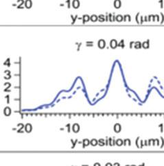
13 sites created by two lasers incident on a circular aperturee can be brought together and separated by tilting the angles of incidence of the laser beams. Figure (3b) shows the light pattern created by two laser beams as they are tilted together from incident angles γ= = + / rad to γ=0 rad [6]. Bringingg two qubit sites close together could pose a problem for quantum computation in that two Rb atoms could unintentiona ally tunnel between traps, likely changing the logical consequences of a qubit gate. The probability of this occurring can be limited by exploiting the interaction of different polarizations of light with atoms in specific hyperfine magnetic substates. As further discussed in the MOT section of this paper, the polarization of a photon is related to the angular momentum of the photon, resulting in polarization dependent selection rules. Similarly, the potential energy of the dipole traps is dependent on the polarization of the trapping light and the magnetic substate of the trapped Rb atom. The probability of two atoms switching traps can be limited by putting the trapped Rb atoms intoo specific magnetic substates and forming the traps using right (σ + ) and left (σ - ) circularlyy polarized light. Potential energy profiles for 87 Rb in the m F =1 and m F =-1 magnetic substates of a F=1 hyperfine state are shown as two traps are brought together for red detuned light in n Figure (3c) and also for blue detuned light in Figure (3d). Figure 3: (a) Diagram of setup (b) Relative intensity of the light field as two traps are brought together (c) Red detuned light potential-energy profile inn the y direction at z=67 μm of F=1 9

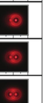
14 m F =1 (solid line) and F=1 m F =-1 (dotted line) (d) Blue detuned light potential-energy profile in the y direction at z=100 μm of F=1 m F =1 (solid line) and F=1 m F = -1 (dotted line) [modified from 6] The polarization dependence of the traps can also be seenn clearly in Figure 4. The intensity pattern of Figure (3b) and Figure (4b) are the same pattern, with two laser beams incident on the circular aperture at γ= = + / rad. Instead of exploringg the intensity pattern as the two lasers are brought together, Figure 4 (c-j) laser light for all the magnetic substates of both the F=1 and the F= =2 shows the potential energy landscape of the diffraction pattern with red detuned hyperfinee states. The column on the right is the cross section of the potential landscape at z=67μm, the location of the outermost bright spot and primary trap for red detuned light. Using the polarization dependence of the trap potential energy in combination with the ability to control the trap position with the angle of incidence γ may enable two qubitss to be brought into close proximity without a great chance of tunneling between traps. This could be beneficial in investigating certain methods of qubit entanglement as well as the implementation of two qubit gates. Figure 4: (a) Diagram of setup (b) Relative light intensityy of diffraction pattern (c)-(j) Potential energy of (b) with red detuned light for the magnetic substates of F= =1 and F=2 hyperfine states [6]. 10

15 The use of the localized bright or dark locations in the diffraction pattern as dipole traps requires the traps to be loadedd with cold atoms in ultra-high vacuum (UHV). Trapping must occur in UHV because any stray atoms in the trapping region cann collide with a trapped atom and knock it out of the trap. The temperature of the atoms loaded into the traps is critical in that the potential energy of the electric field-dipole interaction must be large enough relative to the kinetic energy of the atoms to prevent the atoms from escaping the trap. The lower the temperature of the atoms, the less likely an atom will have enough kinetic energy to escape a trap for a given trapping light intensity. The temperature is also important because of the ability of a stray hot atom to collide with a trapped atom, transferring kinetic energy to it and allowing it to overcome the potential wall. One experimental apparatus frequently used in atomic physics experiments which is able to produce the necessary conditions to load the dipole traps is a magneto-opticachamber. Several experimental complications occur as a result of the traps forming extremely close to the atom trap (MOT), which creates a localized cloud of cold atoms in a vacuum diffracting aperture. Using the traps directly in front of the aperture would require the aperture to be placed inside a vacuum chamber. A vacuum chamber and a cooling system such as a MOT would need to be designed and built specifically for this purpose. Any adjustment or replacement of the aperture would become and immensee task, leading to an overly laborious procedure for any experiment. Instead, the diffraction pattern can be projected from the outside of a vacuum chamber onto a cloud of cold atoms createdd by a MOT, as shown in Figure 5. Computations show a projected trapping site not only cann retain the properties of the original trap, but the projecting optics can also be configured to adjust and optimize the trap size and depth for a particularr experiment. Additionally, projecting the diffraction pattern into the vacuum chamber enable all of the optics to remain outside of the MOT and vacuum chamber, allowing the aperturee to be easily adjusted or replaced [7]. Figure 5: Projection schematic. The lens focal point lies in the diffraction pattern [modified from 8] 11

16 Magneto-O Optical Atom Trap: We are working to construct a MOT, as seen in Figure 6 below, to cool and confine 87 Rb atoms to a localized cloud in our vacuum chamber. The business components of the MOT are three pairs of mutually perpendicular counter propagating laser beams intersecting at the midpoint between two identical electromagnets placed on either side of the glass portion of the vacuum chamber. (a) (b) Electromagnets Vacuum Chamber Laser Beams Figure 6: (a) Picture and (b) Schematic of primary MOT componentss One of the purposes of the three pairs of counter-propagating beams is to cool the Rb dispensed into the vacuum chamber. The temperature of any gas can be statistically related to the RMS speed of the atoms as MS=(3kT/m) 1/2 (2) [23] v RM where k is the Boltzmann constant, T is temperature of the gas in kelvin, and m is the mass of the atoms comprising the gas. The relationship between v and T in this expression shows the temperature of a gas decreases with a decrease in the speed, and therefore momentum, of the atoms comprising the gas. To cool the 87 Rb atoms with the lasers, the frequency of the laser light is red detuned (to a lower frequency) from the resonant frequency of the F=2 F = =3 hyperfinee transition of the 2 S 1/2 2 P 3/2 manifold, as shown in Figure (7a). An atom moving toward a photon from the laser beam will see the frequency of the photon blue shifted (to a higher frequency) due to the optical Doppler shift. If the detuning of the laser is comparable to the increase in frequency due to the optical Doppler shift, the atom will absorb the photon. The atoms moving away from the photons will see the photons as red shifted further below the transition frequency, and therefore will not absorb the photon. The frequency of a photon iss proportional to its energy as well as its momentum. Figure (7b) shows three atoms each with different velocities. The vertical arrow above each atom indicates the energy of the Doppler shifted photon for the velocity of each atom, showing only the atom moving toward the laser beam absorbing a photon. When an atom absorbs a photon and becomes excited, the momentum of the photon will be transferred to the 12

17 atom, decreasing its velocity. The atom will spontaneously emit a photon in a random direction with the same energy and magnitude of momentum as the photon absorbed. Because the photon is emitted in a random direction, the process tends to transfer momentum to the atom in the direction the laser beam is propagating. The process is repeated for many atoms interaction with all three pairs of counter propagating beams, resulting inn a net slowing and cooling of the gas. Laser Beam (a) (b) Figure 7: (a) Detuning from F=2 F =3 transition of the 2 S 1/2 2 P 3/2 manifold (b) Optical Doppler shift of photon energies of atoms with different velocities This cooling technique will work to cool the Rb in the vacuum chamber where the three pairs of counter-propagating lasers intersect, but it will not in itself trap atoms in this region. The trapping function of the MOT emerges from the interaction of the laser light with the atoms in the magnetic field created by the two electromagnets. The two precisely wound identical electromagnets are aligned with opposite polarity at approximately a radius distance apart around the glass portion of the vacuum chamber, as in Figure (8a) below. This configuration of the electromagnets produces a quadrupole field, the strengthh of which increases linearly from B= =0 at the center of the coils (see Figure (8b)). The atoms in thee magnetic quadrupole field experience a Zeeman splitting in the magnetic substates of their energy levels. The change in energy due to the Zeeman effect is proportional to the strength of the magnetic field as well as to the magnetic substate of the electron (3) where EE is the energy shift due to the Zeeman Effect, m F is the magnetic substate, and B is the strength of the magnetic field. Equation (3) applies to the system when B is along the quantization axis of m F. When the magnetic field is alongg the quantization axis, the energy of the states with m F >0 increase with stronger B whereas the energy of the m F <0 statess decrease. When the magnetic field is anti-parallel to the quantization axis, the opposite is true. Utilizing a handy polarization trick, each pair of laser beams consistss of one left circularly polarized (LCP) beam and one right circularly polarized (RCP) beam with respect to the z axis. By convention, discussions involving the quantization axis usually denote the axis of quantization as the z axis, and this does not necessarily reflect the Cartesian z axis of the setup. It will be explicitly stated in this paper when the z axis denotes the Cartesian z axis of a system. 13

18 The helicity of a particle relates the direction of the spin angular momentum to the direction of motion of the particle. It is also related to the right or left nature of a circularly polarized photon, but explicitly relating the helicity and direction of polarization of photons becomes somewhat tricky due to the definition of the quantization axis. The important idea is that the direction of the polarization is related to the direction of the spin angular momentum of a photon. Additional selection rules of the allowed transitions of an electron inn an atom follow from conservation of momentum when the spin of the photon is considered. The selection rules describe the different transitions LCP and RCP photons can cause. In our case with the orientations of RCP and LCP determined with respect to the z axis, RCP photons can only cause a transition between magnetic substatess of m F =1. Similarly, left circularly polarized photons can only can transitions if m F =-1. With the combination of the transition selections rules of the polarized light, the Zeeman splitting of the magnetic substates, and conservation of momentum, the atoms are trapped at the center of the apparatus as described in the example below. (a) (b) B Figure 8: (a) MOT schematic, polarity of electromagnetic coils, and magnetic field B (b) Linear dependence of magnetic field B In studying the workings of a MOT, it is beneficial to examine a simpler case of the interaction of the atoms and circularly polarized light and then extend the same principles to understandd the MOT. Take for example a theoretical atom and the z direction of a quadrupole field (Figure 8a) with incident photons red detuned from an F=0 and F = 1 hyperfine transition. This hyperfine transitionn is present, for instance, in alkali atoms like hydrogen with nuclear spin I=1/2, although it is not the transitionn commonly used when trapping hydrogen. For this example, the z axis denotes both the physical axis chosen as the z axis as well as the quantization axis. When in the external magnetic field, the F =1 state splits into the three energy levels corresponding to m F F=1, 0,-1, linearly diverging from the B=0 center point at z=00 as shown in Figure 9. In the region z>0, the magnetic field is in the +z direction forcing the m F =1 state to increase in energy and the 14

19 m F =-1 state to decrease in energy. In the region where z< <0, B is in the z direction so the energy splitting of the magnetic substates changes in the opposite direction. Figure 9: Zeeman splitting and trapping mechanism of the MOT In this configuration the left circularly polarized photons, labeled -, are incident from the +z direction whereas the right circularly polarized photons + are incident from the -z direction. The further an atom strays from the center in z, the larger the difference in energy levels between m F =1 and m F =-1 becomes. Additionally, the m F =+1 energy level becomes closer to the energy of the red detuned photons, whereas the discrepancy between the m F =-1 energy level and the energy of the photons increases as shown in Figure 9. The + photons, which necessarily cause a transition with m F =+1, travel in thee +z direction. Because of the Zeeman effect, the atom will have a greater probability of absorbing one of these + photons, transferring momentum to the atom in the +z direction. Some time after absorption, the atom will spontaneously emit a photon in a random direction to deexcite. Similarly to the Doppler cooling technique, as the processs continues the net transfer of momentum pushess the atom back to the center. The exact same analysis holds for atoms inn the +z region except the net transfer of momentum is in the z direction, resulting in a configuration which will push any atom back towards the center should it stray from the B= =0 region. A quadrupole field is linear in alll directions from the center and therefore with the correct configuration of light polarization, this concept can be generalized to all three dimensions. A slight complication when analyzing the analogous situation in either the x and y directions in that the magnetic field always points to the center. If the situation is framed such that the quantization axis z can be either the x or the y axis, the magnetic field is in the + z direction when z<0 and is in the z direction when z>0 as can be deduced from Figure (8b). The same mechanism works to confine the atoms at z= 0 with the only difference being that the + photons are incident from the +z direction and the - photons aree incident from the z direction to correspond with the m F states splitting in the opposite fashion than the previous example. Considering the radial symmetryy of the quadrupole field,, the x and y axis can be taken as whichever horizontal directions the laser beams are propagating in the actual experiment. 15

20 In addition to the simplification made by considering an atom in only a single dimension, another significant simplification in the example was the simple energy structure of the theoretical atom. The hyperfine structure of 87 Rb, as seen in Figure 1, is notably more complex than the structure of the theoretical atom in the example. The trapping transition used in practice for 87 Rb is the F=2 F =3 transition of the 2 S1/2 2 P 3/2 manifold. Inn contrast to the theoretical atom s one m F ground state and three m F excited states, 87 Rb has 5 m F ground states and 7 m F excited states. The beauty of the system is that the same processs works to transfer momentum to the atom in the direction of the center of the trap regardless of the additional magnetic substates, but a complication occurs from the relatively low chance of an unintended transition. Granted the trapping laser is precisely tuned slightly to the red of the resonance frequency of the trapping transition, which leads to a high probability for the F=2 F =3 transition as shown in Figure 10, there is a non-zero chance for the electron to be excited into the F =2 state. From the F =2 states, the selection rule F=0, + / - 1 allows the atom to deexcite into the F=1 ground state as will occasionally happen. To resolvee this issue, a pump laserr is incorporated into the system. The pump laser is tuned to the F=1 to F =2 transition of the 2 P 3/2 manifold, which grants the electron a probability to fall back into the needed F=2 ground state, as seen in Figure 10. The process of exciting an atom from the ground state to an excited statee in order for it to eventually decay into a higher hyperfine ground state is a well-established concept in atomic physics called optical pumping. Figure 10: Trap and Pump Laser transitions [22] A crucial aspect of this method of trapping atoms is the precise tuning and stability of the lasers. Intricate feedback and monitoring systems continuously keep the frequency of light emitted from the laserss stable on the set frequency throughh temperature control and small physical adjustments to the lasers. A saturated absorption apparatus is used too find and adjust the system to the exact frequency needed for the correct detuning. The saturatedd absorption apparatus is the topic of the experimental section of this paper. Saturated Absorption: Ordinarily the hyperfine structure of Rb is not immediately apparentt when the absorption spectrum of gaseous Rb is examined. Rubidium will naturally move in all directions with a 16

21 range of velocities when let alone in vacuum. Equation 2 is one result of statistically analyzing this intuitive phenomenon. A range of photon energies can be absorbed by Rb gas in a cell due to the Doppler shifts caused by the different velocities off the atoms, giving rise to a broad peak in the absorption spectrum around a fine structure transition frequency f 0. Doppler peaks, resembling Figure 11, are significant and broad enough to overpower the sharp peaks expected from the hyperfine structure of the atoms. The saturated d absorption apparatus exposes the hyperfinee structure of the atoms within the Doppler peaks from the interaction of two laser beams with the atoms traveling at only certain velocities. Figure 11: Doppler Peak in absorption spectrum around transition frequency f 0 The working part of the saturated absorption apparatus consists of two counter-propagating laser beams of significantly different power passing through a Rb cell. The weaker beam, called the probe beam, acts as the signal with the use of a photodetector as seen in Figure 12. The strong (pump) beam and the probe beam originate from the same laser and are the exact same frequency. The probe beam is split off from the pump beam a short distance from the cell. Althoughh the light transmitted from the pumpp beam is never recorded, the signal from the probe beam transmits information about the combined interaction of both laser beams with the atoms. A saturated absorption scan is performed by scanning a range of frequencies around the 2 S 1/2 2 P 3/2 transition frequency. Without the influencee of the pumpp beam on the atoms, this would result in the photodetector simply recording the Doppler peaks from the probe beam. Figure 12: Saturated absorption schematic 17

22 For this discussion, allow the direction the lasers propagate to be denoted as the z axis, with the direction of the pump beam as +. The hyperfine structure of Rb is found by scanning a range of laser light frequencies around the frequency corresponding to the 2 S 1/2 2 P 3/2 transition. Only the signal from the probe beam is recorded, so the atoms which interact with the probe beam are the atoms critical to understanding how a saturated absorption apparatus works. Atoms with velocities in the +z direction, v z >0, will see the probe beam frequency blue shifted up to a higher frequency. When the laser light frequency approaches and is slightly lower than a transition frequency during a scan, atoms with some v z >0 will see the probe beam frequency shifted up to the transition frequency and will absorb photons. The decrease in intensity of the beam is seen with the photodetector. The atoms with v z >0 able to absorb probe beam photons will see the photons from the pump beam red shifted further away from the transition frequency because they are moving away from the pump beam. The pump beam photons are therefore less likely to be absorbed by these atoms. Similarly, when the laser light frequency is slightly above the transition frequency, atoms with some v z <0 will see the probe beam red shifted down to the transition frequency and will absorb photons, decreasing the intensity of the probe beam on the photodetector. The frequency of the pump beam photons will appear blue shifted further above the transition frequency to the atoms, and again are less likely to be absorbed. Omitting the interaction of the laser beams atoms with v z =0, the resulting intensity curve read by the photodetector would simply be a Doppler peak. The Doppler peak in Figure 11 can be thought of as a plot of as intensity vs frequency. Saturated absorption works to distinguish the hyperfine structure of rubidium within the Doppler peaks by capitalizing on the interaction of the atoms with v z =0. Granted these atoms may have velocities in x and y, there will be no Doppler shift of the photon frequencies of either the pump or probe beams to the atoms because they are not moving along the axis the laser beams propagate. When the frequency of the beams is in resonance with one of the hyperfine transitions of the atoms, the high intensity pump beam will excite all of the atoms with v z =0. The transition will be saturated; that is, all of the valence electrons in these atoms will be in the 2 P 3/2 manifold. With the transition saturated, the gas will be transparent to the probe beam, resulting in a strong photodetector signal in the middle of the Doppler peak. The induced transparency of the gas perceived by the probe beam due to the saturated transition is the fundamental physics of any saturated absorption apparatus. The counter-propagating beams force the saturation of the transition to occur when the laser light frequency is at a natural transition frequency, providing information not only about the hyperfine structure of rubidium but also information on how to obtain the desired output frequency from the laser. The transition is saturated for the probe beam only for the atoms with v z =0 and when the laser light is resonant with one of the hyperfine transition, eliminating Doppler broadening for the transitions of these atoms. A slight complication arises when the pump and probe beams can excite the same moving atoms, which can occur in between two transition frequencies. Take for instance an atom moving with v z >0, blue shifting the probe beam frequency while red shifting the pump beam frequency. Let the amount the laser frequency is shifted by the velocity of the atom be ω s. If the moving atom is in resonance with the pump beam then 18

23 where ω L is the frequency of the laser light, and ω 1 is the transition frequency. If the Doppler shifted probe beam frequency beam also corresponds to one of the hyperfine transition frequencies of the same atom then where ω 2 is another hyperfine transition frequency. Combining these two equation and solving for ω L, 2 (4) We find it is possible to see the saturated absorption effect for some atoms at laser frequencies halfway between two hyperfine transition frequencies [21]. Fortunately, the saturated absorption spectrum has been studied extensively, allowing the identification of the hyperfine peaks in the saturated absorption spectrum of rubidium with relative ease. Chapter 3: Experiment: Overview: In order to understand the workings of our saturated absorption apparatus, a word should be first said about how the lasers work. Three major sensitive variables change the frequency of light emitted from the laser: temperature, current through the laser diode, and the position of the diffraction grating. The temperature of the lasers is maintained precisely with a fluid heat sink system and thermoelectric coolers (TEC). Two Thermo Scientific NESLAB RTE 7 refrigerated baths continuously pump water at a set temperature (typically 15 C) through the base of the lasers, acting as a heat sink and dissipating any unwanted thermal energy from the system. Each laser also contains two TEC s, which can transfer thermal energy to the heat sink or add thermal energy to the laser diode platform to precisely maintain the laser diode at a set temperature. The TEC s are controlled with Thorlabs ITC-502 laser controllers which provide a high level of thermal stability and decouple the temperature of the lasers from the environment, while allowing controlled manipulation of the temperature for tuning. The current through the laser diode I LD plays an immense role in the frequency of light emitted from the laser, allowing it to be used as the coarse adjustment parameter for the laser light frequency. It is manually controlled with the same Thorlabs laser controllers that control the TEC s. The laser controllers are designed to maintain a set I LD with high precision, helping to prevent any unwanted change in laser light frequency. The lasers used for this experiment are external cavity lasers, which use several optics to adjust the properties of the light emitted from the laser diode. The primary component affecting the laser light is a diffraction grating, which is the first optic the light is incident upon after being emitted from the laser diode, as seen in Figure 13. Some of the light incident on the diffraction grating is reflected back to the laser diode, causing the laser diode to emit the same frequency light as the reflected beam. The frequency of the reflected beam is dependent on the angle of incidence θ of the laser diode output beam on the diffraction grating. Altering θ changes the frequency of light reflected back to the laser diode and therefore the frequency of light emitted from the laser. The frequency of the lasers can thus be finely tuned by controlling the angle of the diffraction grating, which is done with a piezoelectric transducer, or piezo. The piezo is 19

24 useful in rotating the diffraction grating because piezoelectric materials expand when a voltage is applied across it. The scan of light frequencies needed for the saturated absorption proceduree is performed by applying a voltage ramp to the piezo connected to one edge of the diffraction grating mount, whichh causes a rotation in the diffraction grating and a range of frequencies of light to be emitted from the laser. Figure 13: Laser Schematic [modified from 22] Our saturated absorption setup consists of three mirrors, a 90/10 beam splitter, a 50/50 beamsplitter, the Rb vapor cell, a photodetector, a Thorlabs MC1000A optical chopper (beam chopper), two irises for beam alignment, and a Stanford Reseach Systems SR810 DSP lock-idata to a amplifier (LIA) which analyzes the signal from the photodetector and sends the computer. The 90/10 beam splitter transmits 90% of the incident beam and reflects 10%, while the 50/500 intuitively both transmits and reflects 50% of the incident beam. A schematic of the setup is shown in Figure 14. The general theory for saturated absorption as discussed in Chapter 2 applies to this setup, but our setup deviates slightly from the workings of traditional saturated absorption in our use of the beam chopper and lock-in amplifier. The beam chopper is a disc with wide spokes used to periodically block a laser beam, creating pulses of the beam. The frequency with whichh the beam is chopped is controlled with a beam chopper controller, which also sends a signal to the LIA indicating the chopping frequency. The function of the LIA is to analyze an input (photodetector) signal with respect to a reference frequency (chopping frequency). The LIA performs mathematical functions too extract the portions of the input signal modulated at the reference frequency. We use a computer to read the output of the LIA and gain valuable informationn correlating the voltage applied to the piezo with the frequency of the laser beams that cause each of the hyperfine transitions of Rb.. With the use of the LIA in the saturated absorption setup, a scan of laser light frequencies around the transition frequency will not show a traditional Doppler peak with hyperfine transition spikes of intensity. Although the physics of the laser-atom interactions are the same as described in chapter 2, the LIA works to expose the hyperfine structure of Rb by filtering out unwanted portions of the photodetector signal. The beam chopper is used to create pulses of the pumpp beam before it is incident on the vapor cell. The LIA keeps the signal from the photodetector when the probe beam is modulated at the same frequencyy as the chopping frequency. In other words, the LIA looks for signal from the probe beam which is incoming at the same frequency as 20

25 the frequency with which the pump beam is chopped. This occurs when both beams interactt with the same atoms. As previously described, the probe beam will be transmitted throughh the cell with a high intensity when the frequency of the lasers is on a hyperfine transitionn because the pump beam saturates the transition of v z =0 atoms. The pump beam gets chopped near 280Hz, resulting in pump laser pulses to interact with the atoms in the cell about once every 4ms. When the laser light frequency is on transition, the probe beam will see the cell become transparent approximately every 4ms when the pulse of pump beam saturates the transition, resulting in a strong signal to the photodetector r. The scan of frequencies is performed with the use of a LabVIEW program. The LabVIEW program is designed to be able to output an adjustable voltage ramp to the piezo, with the voltage ramp able to range from -10V to +10V. The period of the ramp is also adjustable and can range from 30s to 90s for a typical scan. The longer the scan time, the longer the laser frequency will correspond to each transition frequency in the Doppler peak, allowing the LIA to collect more data and generally produce better results. Scans as quick as 30s can potentially show the saturated absorption effect and reveal the hyperfine structure of an atom becausee the light pulses are incident on the atoms about once every 4ms, which can be rapid enough for the LIA to collect a sufficient amount of data while the laser light iss resonant with the transition. Figure 14: Saturated Absorption Schematic 21

26 One more note should be made about an additional intricacy of the setup. The vapor cell contains two isotopes of Rb, 87 Rb and 85 Rb. As previously mentioned, this experiment uses 87 Rb with nuclear spin I=3/2. The isotope 85 Rb is the more abundant isotope in nature and has a nuclear spin I=5/2, leading to a slightly more complicated and energetically different hyperfine structure than that of 87 Rb. The difference in energy of the hyperfine structures results in the peaks from both the isotopes to be present in a scan of the absorption spectrum of the vapor cell. The difference in relative abundance of the isotopes at times can be used to differentiate between the peaks of 87 Rb and 85 Rb. The data collected through previous studies of Rb can be used along with frequency markers from a Fabry-Perot interferometer to accurately to differentiate between the peaks of 87 Rb and 85 Rb, as well as identify the false hyperfine peaks described by equation (4). Alignment: Procedure: The alignment of the laser beams is critical for the saturated absorption procedure to work correctly. The closer the beams are to being truly counter propagating, the stronger the signal response will be when the laser light frequency is on transition. The best ways to align the setup is to first perform a rough alignment and subsequently precisely align the beams. As with many optics experiments, quality alignment of the beams can take practice and a significant amount of tinkering. There is no perfect cookbook for perfect alignment, but these guidelines help with quality alignment. General Tips: Try and align the beams along the bolt lines of the optics table. It is easy for a beam to be clipped on the side of an optic, reducing the intensity of a beam and likely hindering the performance of the setup. When the optics are configured to create beam paths along the bolt lines, the lasers are incident and reflected at 45 angles, reducing clipping and helping with ease of alignment. If possible, it is always good to center the beam on an optic during rough alignment allowing more space for beam movement in future adjustments. If the setup needs a large change in alignment, remove the Rb vapor cell. The following procedure assumes the vapor cell is removed. The flashlights can be used to block a beam while the other beam is being aligned. Rough Alignment: Note: Optics are referred to by labels as indicated in Figure Align the incoming laser beam onto mirror A 2. Roughly align the probe beam on path BCD Both the position and angles of optics may need to be adjusted. Check for beam getting clipped on posts on B. Alignment to the point of the beam hitting all optics B,C, and D is sufficient for this rough alignment. 22

27 3. Roughly align the pump beam on path BED Both the position and angles of optics may need to be adjusted. Minimize any clipping occurring on the edges of E Alignment to the point of the beam hitting all optics B,E, and D is sufficient for this rough alignment. 4. Return to the alignment of BCD and align beam path such that the beam is incident near the center of each optic. The same should be done for beam path BED. Repeat until alignment of each beam is incident on each optic near the center and about at a 45 angle. Even though one branch of the laser paths is meant to be transmitted directly though the 90/10 beamsplitter B, both path directions are dependent on the position of B. Once the optics are configured such that the pump and probe beams are incident around the centers of E and C respectively, B should be set and left alone if possible. While possibly seeming tedious, this can save significant amounts of time during the fine alignment and potentially prevent the need for the alignment procedure to start over. 5. Place Rb cell in the beam path between E and D with the beam incident near the center of the cell 6. Adjust E and the position of the cell such that the beam goes through the center of the cell and hits D, and vice versa. The beam often can hit side of cell, which obscures the beam path. Fine Alignment: 1. Place the two irises near D and E, with the iris in the large square mount near E. Place the cameras near Q and P pointed in the +z direction to observe the pump beam on the irises. The irises P and Q should be placed close to D and E because the larger the distance between them, the more precisely the beams must be anti-parallel to go through both irises. The iris with the large square frame is better used for iris Q during the alignment of the probe beam. 2. Align the irises to the pump beam. The path of the pump beam can only be changed with E, whereas the path of the probe beam can be adjusted with both C and D. The additional degrees of freedom for adjusting path of the probe beam indicates that the irises should be aligned with the pump beam, and subsequently aligning the probe beam to match the path of the pump beam The position of each iris should be adjusted such that the center of the pump beam is at the center of the iris. The shape of the beam is not perfectly circular, so this alignment is somewhat of a judgment call, but the most important part of the beam is the center bright portion with the outer fringe portion contributing less to the saturated absorption signal. Centering the iris and the beam can be done both with translating the position of the iris as well as changing the angle of E, but changing the angle of E should be reserved for fine adjustments because it affects the alignment of the beam with both P and Q 23

28 The angle of the CCD cameras affects thee image. Place the cameras as straight as possible. 3. Align the probe beam to the irises. It can be helpful to think the of function of mirror C as to position the point of incidence of the beam on D such that when reflected it will be centered on iris P. Mirror D controls the angle of propagation of the beam and can be thought of as primarily serving to align the beam with Q. Change position of cameras to see beam the position on irises First align the beam with iris Q with P open. When P is closed, the offset of the beam from the center of P determines the adjustment needed for the position of the beam s incidence on D. Adjust C accordingly. Realign the beam with the center of P. Open P and observe the position of the beam with respect to the center of Q. Adjust D accordingly. Close P and repeat. See figure 15. (a) (b) Figure 15: (a) Changing of position of beam on D by adjusting C (b) Changing direction of beam by adjusting D 4. Place photodetector behind E 24

29 Instrumentation and Settings: Several of the instruments used in the saturated absorption procedure have a variety of settings that must be configured and considered when performing the saturated absorption procedure. The lock-in amplifier has many different setting that can affect how it reads the input and how it operates on the input signal to construct an output signal. The output signal of the LIA is given by 1 10 (5) where X is the input signal. More details of each of the variables in equation (5) variable can be found on page 4-13 of the LIA manual. The integration time τ is an important variable that affects how the LIA processes the data. In general longer integration times make the LIA average over more cycles of input data, which affects the sensitivity of the output. Longer integration times tend to reduce the amount of noise, but if the integration time is too long the hyperfine peaks may be averaged out of the signal. The best integration time for the scans performed was found to be τ=100ms, limiting the amount of noise in the signal while keeping the sharpest hyperfine peaks possible. The function of the chopper controller is fairly straight forward, but one of the two mode settings can cause the reference frequency to be communicated incorrectly with the LIA. The mode needed for our experiment is denoted 5Yn on the LED display. The mode setting can be changed by first selecting the mode menu, as seen with the LEDs, by pressing the mode button and then changing the setting with cycle. This setting is the constant frequency setting. One more complication with the beam chopper is that the frequency setting cannot be an integer multiple of 60, 60 Hz(6) where n=1,2,3 primarily because the power grid oscillates as 60 Hz, increasing the susceptibly of LIA signal electrical noise. As previously mentioned, the experiment is controlled with the computer using LabVIEW. The LabVIEW V.I. (program) Ramp Program Andy.vi is able to monitor and record four data inputs while outputting an adjustable voltage ramp. The voltage ramp can run between any two voltages from -10V to +10V at an adjustable speed. The program is able to output the voltage ramp to different DAQ board output channels, but as of the writing of this paper the setup is configured such that the control panel output 0 sends the ramp through the lock box to the piezo in the laser. The program is able to display up to four inputs on graphs in real time, graphing the input voltage vs. the ramp voltage. The scale of the graphs is dictated by the channel input on the control panel as opposed to the overlay input, which simply shows the shape of the overlay channel on the same graph. Due to some of the coding of the program, the control panel input numbers are not the exact DAQ board analog input numbers. The relationship between the input numbers and analog channel numbers is displayed in Table 2 below. When the control panel input is -1, LabVIEW does not display any analog channel from the DAQ board in that particular graph. 25

30 Control Panel Input Analog Channel 1 NO INPUT Table 2: Control panel input and analog channel The control panel contains a dialogue text box used in naming the data file of a saved scan. The program uses the text entered in the dialogue box at the start of the scan to name the file. Any changes of text in the dialogue box during a scan do not affect the name of the data file for that scan. The name of the data file created also contains a four digit number which automatically is increased with every saved scan to prevent overwriting any data. The number displayed is increased when the scan starts, and the increased number is the number used in the file name. In other words, the name of a file is created using the text in the dialogue box when the scan is started in combination with the increased number displayed after the scan starts. This slightly confusing saving process contributed to incorrect descriptions of the scan properties in the file names for the data presented in this paper, corresponding to the data files D0003- to D Troubleshooting: Many things can prevent the setup from functioning correctly. Although some of these troubleshooting suggestions may seem obvious, simple straightforward mistakes become easier to make as the experiment becomes more complicated. These are some common problems that may cause the setup to not function correctly even when the beams are sufficiently aligned. If a scan is run but no saturated absorption signal is found check the following: All the correct cords are plugged in (check DAQ board) Everything is turned on (PHOTODIODE and LOCK BOX) Nothing is blocking the beam path to the photodetector The lock box is set to comp for the ramp setting The LabVIEW program is set to output 0 Display channels on LabVIEW program Settings of LIA Atom fluorescence, visually and with oscilloscope Results: The saturated absorption scans performed are of the Rb transition with temperature T=14.996kΩ, I LD =111.30mA, at a chopping frequency of f=279hz. The laser beam used for saturated absorption is split into two branches prior to the saturated absorption apparatus, the second branch passing through a separate vapor cell and used as part of a laser locking feedback system 26

31 called a dichroic atomic vapor laser lock (DAVLL). Thee error signal between two photodetectors in the feedback system is often observed alongside the saturated absorption scan to compare the absorption spectrum of the Rb with the saturated absorption data. The graph below shows the saturated absorption curve from peaks from both 877 Rb and 85 Rb for a 60s scan and integration time (labeled time constant on the LIA front panel) of τ=100ms along with the absorption curve (error) from the DAVLL photodetectors. Figure 16: Saturated Absorption Curve τ=100ms Saturated absorption scans were performed with LIA integration time varying from τ=10ms to τ=300ms, resulting in the observation that the optimum integration time is τ=100ms when the chopping frequency is f=279hz. Figure 17 shows the effects of integration time on the saturated absorption curve. Figure 17: Saturated Absorption Curves with integrationn times (a) τ= =30ms (b) τ= =100ms and (c) τ=300mss 27

32 Along with the integration time of the LIA, the range of the voltage ramp and ramp period P are two easily adjustable settings on the LabVIEW ramp program whichh influence the precision of the saturated absorption data recorded. The ramp program is coded to record 1000 data points regardless of the range of ramp voltage and period, meaning that the transition peaks can be resolved more acutely by limiting the range of the ramp voltage. The period P of the scan can influencee the precision of the scan by allowing the LIA to collect more data. Figure 18 below shows the saturated absorption curves from 60s second scans of both the 87 Rb and 85 Rb transitions with integration time τ=100ms. Figure 18: Saturated Absorption Curves P=60s, τ=100ms Similarly, the effects of the changing the voltage ramp period can be seen in by comparing the curves in Figure 19, one of whichh has P=30s and P=60s. 28