March 25, 2010 CHAPTER 2: LIMITS AND CONTINUITY OF FUNCTIONS IN EUCLIDEAN SPACE

Transcription

1 March 25, 2010 CHAPTER 2: LIMIT AND CONTINUITY OF FUNCTION IN EUCLIDEAN PACE 1. calar product in R n Definition 1.1. Given x = (x 1,..., x n ), y = (y 1,..., y n ) R n,we define their scalar product as n x y = x, y = x i y i Example 1.2. (2, 1, 3) ( 1, 0, 2) = = 4 Remark 1.3. x y = y x. Definition 1.4. Given x = (x 1,, x n ) R n we define its norm as x = x x = x x2 n Example 1.5. Example: ( 1, 0, 3) = 10 i=1 Remark 1.6. ome interpretations of the norm are: The norm x is the distance from x to the origin. We may also interpret x as the length of the vector x. The norm x y is the distance between x and y. Remark 1.7. Let θ be the angle between u and v. Then, cos θ = u v u v The Euclidean space R n Definition 2.1. Given p R n and r > 0 we define the open ball of center p and radius r as the set B(p, r) = {y R n : p y < r} and the closed ball of center p and radius r as the set B(p, r) = {y R n : p y r} Remark 2.2. Recall that p y is distance from p to y. For n = 1, we have that B(p, r) = (p r, p + r) and B(p, r) = [p r, p + r]. 1

2 2 CHAPTER 2: LIMIT AND CONTINUITY OF FUNCTION IN EUCLIDEAN PACE [ ] ( ) p - r p p + r p - r p p + r B(p,r) B(p,r) For n = 2, 3 the closed balls are n = 2 n = 3 For n = 2, 3 the open balls are n = 2 n = 3 Definition 2.3. Let R n. We say that p R n is interior to if there is some r > 0 such that B(p, r). Notation: is set of interior points of. Remark 2.4. Note that because p B(p, r) for any r > 0. Example 2.5. Consider R 2, = [1, 2] [1, 2]. Then, = (1, 2) (1, 2).

3 CHAPTER 2: LIMIT AND CONTINUITY OF FUNCTION IN EUCLIDEAN PACE º Example 2.6. Consider = [ 1, 1] {3} R. Then, = ( 1, 1). [ º ] ( ) Definition 2.7. A subset R n is open if = Example 2.8. In R, the set = ( 1, 1) is open, T = ( 1, 1] is not. ( ) ( T ] º = T º = ( ) Example 2.9. The set = {(x, 0) : 1 < x < 1} is not open in R 2. ( ( )) ( ) n = 1 n = 2

4 4 CHAPTER 2: LIMIT AND CONTINUITY OF FUNCTION IN EUCLIDEAN PACE You should compare this with the previous example Example The open ball B(p, r) is an open set. Example The closed ball B(p, r) is not an open set, because B(p, r)= B(p, r). B(p,r) º B(p,r) = B(p,r) Example Consider the set = {(x, y) R 2 : x 2 + y 2 1, x y}. Then, = {(x, y) R 2 : x 2 + y 2 < 1, x y}. o, is not open. º Proposition is the largest open set contained in. (That is is open, and if A is open, then A ). Definition Let R n. A point p R n is in the closure of if for any r > 0 we have that B(p, r). Notation: is the set of points in the closure of. Example Consider the set = [1, 2) R. Then, the points 1, 2. But, 3 /.

5 CHAPTER 2: LIMIT AND CONTINUITY OF FUNCTION IN EUCLIDEAN PACE 5 [ ) ( ) Example Consider the set = B ((0, 0), 1) R 2. Then, the point (1, 0). But, the point (1, 1) /. (1,1) (1,0) Example Let = [0, 1], T = (0, 1). Then, = T = [0, 1]. Example Let = {(x, y) R 2 : x 2 + y 2 1, x y}. Then, = B ((0, 0), 1). Example B(p, r) is the closure of the open unit ball B(p, r). Remark Definition A set F R n is closed if F = F. Proposition A set F R n is closed if and only if R n \ F is open. Example The set [1, 2] R is closed. But, the set [1, 2) R is not. Example The set B(p, r)is closed. But, the set B(p, r) is not. Example The set = {(x, y) R 2 : x 2 + y 2 1, x y}is not closed. Proposition The closure of is the smallest closed set that contains. (That is is closed, and if F is another closed set that contains, then F ). Definition Let R n, we say that p R n is a boundary point of if for any positive radius r > 0, we have that, (1) B(p, r). (2) B(p, r) (R n \ ). Notation: The set of boundary points of is denoted by.

6 6 CHAPTER 2: LIMIT AND CONTINUITY OF FUNCTION IN EUCLIDEAN PACE Example Let = [1, 2), T = (1, 2). Then, = T = {1, 2}. [ ) 1 2 ( T ) 1 2 = 1 2 T Example Let = [ 1, 1] {3} R. Then, = { 1, 1, 3}. [ ] Example Let R 2, = [1, 2] [1, 2]. Then, is Example = {(x, y) R 2 : x 2 + y 2 1, x y}. Then, = {(x, y) : x 2 + y 2 = 1} {(x, y) R 2 : x 2 + y 2 1, x = y}. The above concepts are related in the following Proposition. Proposition Let R n, then (1) = \ (2) = (3) = R n \. (4) is closed = (5) is open = =. Proposition (1) The finite intersection of open (closed) sets is also open (closed). (2) The finite union of open (closed) sets is also open (closed).

7 CHAPTER 2: LIMIT AND CONTINUITY OF FUNCTION IN EUCLIDEAN PACE 7 Definition A set R n is bounded if there is some R > 0 such that B(0, R). Example The straight line V = {(x, y, z) R 3 : x y = 0, z = 0} is not a bounded set. Example The ball B(p, R) of center p and radius R is bounded. Definition A subset R n is compact if is closed and bounded. Example = {(x, y) R 2 : x 2 + y 2 1, x y} is not compact (bounded, but not closed). Example B(p, R) is not compact (bounded, but not closed). Example B(p, R) is compact. Example (0, 1] is not compact. [0, 1] is compact. Example [0, 1] [0, 1] is compact. Definition A subset R n is convex if for any x, y and λ [0, 1] we have that λ x + (1 λ) y. Example Let A a matrix of order n m and let b R m. We define = {x R n : Ax = b} as the set of solutions of the linear system of equations Ax = b. Let x, y, be two solutions of this linear system of equations. Then, we have that Ax = Ay = b. If we now take any 0 t 1 (indeed any t R) then A(tx + (1 t)y) = tax + (1 t)ay = tb + (1 t)b = b that is, tx + (1 t)y so the set of solutions of a linear system of equations is a convex set. Example {(x, y) R 2 : x 2 + y 2 1, x y} is not a convex set. x y

8 8 CHAPTER 2: LIMIT AND CONTINUITY OF FUNCTION IN EUCLIDEAN PACE We study now functions f : R n R 3. Function of several variables Example 3.1. f : R 2 R defined by f(x, y) = x + y 1 also f : R 3 R defined by f(x, y) = x sin y also f : R 4 R defined by f(x, y, z) = x 2 + y z 2 f(x, y, z) = z exp x 2 + y 2 f(x, y, z, t) = sin x + y + z exp t. Occasionally, we will consider functions f : R n R m like, for example, f : R 3 R 2 defined by f(x, y, z) = (x exp y + sin z, x 2 + y 2 z 2 ) But, if we write f(x, y, z) = (f 1 (x, y, z), f 2 (x, y, z)) with f 1 (x, y, z) = x exp y + sin z, f 2 (x, y, z) = x 2 + y 2 z 2 Then, f(x, y, z) = (f 1 (x, y, z), f 2 (x, y, z)). o, we may just focus on functions f : R n R. Remark 3.2. When we write x + y + 1 f(x, y, z) = x 1 it is understood that x 1. That is the expression of f defines implicitly the domain of the function. For example, for the above function we need that x + y and x 1. o, we assume implicitely that the domain of f(x, y, z) = x+y+1 x 1 is the set D = {(x, y) R 2 : x + y 1, x 1} Usually we will write f : D R n R to make explicit the domain of f. Definition 3.3. Given f : D R n R we define the graph of f as G(f) = {(x, y) R n+1 : y = f(x), x D} Remark that the graph can be drawn only for n = 1, 2. Example 3.4. The graph of f(x, y) = x 2 + y 2 is

9 CHAPTER 2: LIMIT AND CONTINUITY OF FUNCTION IN EUCLIDEAN PACE 9 Example 3.5. The graph of f(x, y) = x 2 y 2 is Example 3.6. The graph of f(x, y) = 2x + 3y is

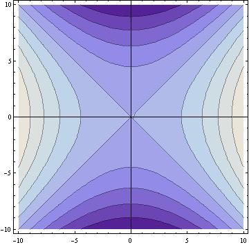
10 10 CHAPTER 2: LIMIT AND CONTINUITY OF FUNCTION IN EUCLIDEAN PACE 4. Level curves and level surfaces Definition 4.1. Given f : D R n R and k R we define the level surface of f as the set C k = {x D : f(x) = k}. If n = 2, the level surface is called a level curve. Example 4.2. The level curves of f(x, y) = x 2 + y 2 are The arrows point in the direction in which the function f grows. Example 4.3. The level curves of f(x, y) = x 2 y 2 are The arrows point in the direction in which the function f grows. Example 4.4. The level curves of f(x, y) = 2x + 3y are

11 CHAPTER 2: LIMIT AND CONTINUITY OF FUNCTION IN EUCLIDEAN PACE 11 The arrows point in the direction in which the function f grows. 5. Limits and continuity Definition 5.1. Let f : D R n R and let L R, p R n. We say that lim f(x) = L x p if given ε > 0 there is some δ > 0 such that f(x) L < ε whenever 0 < x p < δ. This is the natural generalization of the concept of limit for one-variable functions to functions of several variables, once we remark that the distance in R is replaced by the distance in R n ). Note that interpretation is the same, i.e., x y is the distance from x to y in R and x y is the distance from x to y in R n. Proposition 5.2. Let f : R n R and suppose there are two numbers, L 1 and L 2 that satisfy the above definition of limit. That is, L 1 = lim x p f(x) and L 2 = lim x p f(x). Then, L 1 = L 2 Remark 5.3. The calculus of limits with several variables is more complicated than the calculus of limits with one variable. Example 5.4. Consider the function f(x, y) = { (x 2 + y 2 ) cos( 1 x 2 +y 2 ) if (x, y) (0, 0), 0 if (x, y) = (0, 0).

12 12 CHAPTER 2: LIMIT AND CONTINUITY OF FUNCTION IN EUCLIDEAN PACE We will show that lim f(x, y) = 0 (x,y) (0,0) In the above definition of limit we take L = 0, p = (0, 0). We have to show that given ε > 0 there is some δ > 0 such that whenever 0 < (x, y) < δ, where f(x, y) < ε (x, y) = x 2 + y 2 o, fix ε > 0 and take δ = ε > 0. uppose that then, 0 < (x, y) = x 2 + y 2 < δ = ε x 2 + y 2 < ε and (x, y) (0, 0) so, f(x, y) = (x2 + y 2 1 ) cos( x 2 + y 2 ) < ε 1 cos( x 2 + y 2 ) ε where we have used that cos(z) 1 for any z R. It follows that lim (x,y) (0,0) f(x, y) = 0. Remark 5.5. The above definition of limit needs to be modified to take care of the case in which there are no points x D (where D is the domain of f) such that 0 < p x < δ For example, what is lim x 1 ln(x)? To avoid formal complication, we will only study lim x p f(x) for the cases in which the set {x D : 0 < p x < δ}, for every δ > 0 Definition 5.6. : A map σ(t) : (a, b) R n is called a curve in R n. Example 5.7. σ(t) = (2t, t + 1), t R.

13 CHAPTER 2: LIMIT AND CONTINUITY OF FUNCTION IN EUCLIDEAN PACE Example 5.8. σ(t) = (cos(t), sin(t)), t R Example 5.9. σ(t) = (cos(t), sin(t), t), σ : R R Proposition Let p D R n and f : D R n R. Consider a curve σ : [ ε, ε] D such that σ(t) p whenever t 0 and lim t 0 σ(t) = p. uppose, lim x p f(x) = L. Then, lim t 0 f(σ(t)) = L Remark The previous proposition is useful to prove that a limit does not exist or to compute that value of the limit if we know in advance that the limit exists. But, it cannot be used to prove that a limit exists since one of the hypotheses of the proposition is that the limit exists. Remark Let f : D R 2 R. Let p = (a, b) consider the following particular curves σ 1 (t) = (a + t, b) Note that so, if then, we must also have σ 2 (t) = (a, b + t) lim σ i(t) = (a, b) i = 1, 2 t 0 lim f(x, y) = L (x,y) (a,b) lim f(x, b) = lim f(a, y) = L x a y b

14 14 CHAPTER 2: LIMIT AND CONTINUITY OF FUNCTION IN EUCLIDEAN PACE Remark Iterated limits uppose that lim (x,y) (a,b) f(x, y) = L and that the following one-dimensional limits lim f(x, y) x a f(x, y) lim y b exist for (x, y) in a ball B((a, b), R). Define the functions g 1 (y) = lim x a f(x, y) g 2 (x) = lim y b f(x, y) Then, ( lim x a lim y b ) f(x, y) = lim g 2 (x) = L x a lim y b ( ) lim f(x, y) = lim g 1 (y) = L x a y b Again, this has applications to compute the value of a limit if we know beforehand that it exists. Also, if for some function f(x, y) we can prove that lim lim f(x, y) lim lim f(x, y) x a y b y b x a then lim (x,y) (a,b) f(x, y) does not exist. But, the above relations cannot be used to prove that lim (x,y) (a,b) f(x, y) exists. Example Consider the function, f(x, y) = { x 2 y 2 x 2 +y 2 if (x, y) (0, 0), 0 if (x, y) = (0, 0).

15 CHAPTER 2: LIMIT AND CONTINUITY OF FUNCTION IN EUCLIDEAN PACE 15 Note that lim lim x 2 f(x, y) = lim f(x, 0) = lim x 0 y 0 x 0 x 0 x 2 = 1 but, lim lim y 2 f(x, y) = lim f(0, y) = lim y 0 x 0 y 0 y 0 y 2 = 1 Hence, the limit x 2 y 2 lim (x,y) (0,0) x 2 + y 2 does not exist. Example Consider the function, f(x, y) = { xy x 2 +y 2 if (x, y) (0, 0), 0 if (x, y) = (0, 0).

16 16 CHAPTER 2: LIMIT AND CONTINUITY OF FUNCTION IN EUCLIDEAN PACE Note that the iterated limits lim lim f(x, y) = lim x 0 y 0 x 0 lim lim f(x, y) = lim y 0 x 0 y 0 0 x 2 = 0 0 y 2 = 0 coincide. But, if we consider the curve, σ(t) = (t, t) and compute lim t 0 f(σ(t)) = lim f(t, t) = lim t 0 t 0 t 2 2t 2 = 1 2 does not coincide with the value of the iterated limits. Hence, the limit lim (x,y) (0,0) xy x 2 + y 2 does not exist. Example Let f(x, y) = { y if x > 0 y if x 0

17 CHAPTER 2: LIMIT AND CONTINUITY OF FUNCTION IN EUCLIDEAN PACE 17 We show first that lim (x,y) (0,0) f(x, y) = 0. To do this, consider any ε > 0 and take δ = ε. Now, if 0 < (x, y) = x 2 + y 2 < δ then, f(x, y) 0 = y = y 2 x 2 + y 2 < δ = ε Hence, lim f(x, y) = 0 (x,y) (0,0) But, we remark that lim x 0 f(x, y) does not exist for y 0. This so, because if y 0 then the limits lim f(x, y) = y x 0 + lim f(x, y) = y x 0 do not coincide. o, lim x 0 f(x, y) does not exist for y 0. Example Consider the function, f(x, y) = { x 2 y x 4 +y 2 if (x, y) (0, 0), 0 if (x, y) = (0, 0). whose graph is the following

18 18 CHAPTER 2: LIMIT AND CONTINUITY OF FUNCTION IN EUCLIDEAN PACE but, Note that lim lim 0 f(x, y) = lim f(x, 0) = lim x 0 y 0 x 0 x 0 x 4 = 0 lim lim 0 f(x, y) = lim f(0, y) = lim y 0 x 0 y 0 y 0 y 2 = 0 Moreover, if we consider the curve σ(t) = (t, t) and compute t 3 lim f(t, t) = lim f(t, t) = lim t 0 t 0 t 0 t 4 + t 2 = 0 we see that it coincides with the value of the iterated limits. Hence, one could wrongly conclude that the limit exists and lim (x,y) (0,0) x 2 y x 4 + y 2 = 0 But this is not true...because, if we now consider the curve σ(t) = (t, t 2 ) and compute lim f(t, t 0 t2 ) = lim f(t, t 2 ) = lim x 0 t 4 + t 4 = 1 2 Therefore, the limit x 2 y lim (x,y) (0,0) x 4 + y 2 does not exist. t 0 t 4 Theorem 5.18 (Algebra of limits). Consider two funcions f, g : D R n R and suppose lim f(x) = L 1, lim g(x) = L 2 x p x p Then, (1) lim x p (f(x) + g(x)) = L 1 + L 2. (2) lim x p (f(x) g(x)) = L 1 L 2.

19 CHAPTER 2: LIMIT AND CONTINUITY OF FUNCTION IN EUCLIDEAN PACE 19 (3) lim x p f(x)g(x) = L 1 L 2. (4) If a R then lim x p af(x) = al 1. (5) If, in addition, L 2 0, then f(x) lim x p g(x) = L 1 L 2 6. Continuous Functions Definition 6.1. A function f : D R n R m is continuous at a point p D if lim x p f(x) = f(p). We say that f is continuous on D if its continuous at every point p D. Remark 6.2. Note that a function f : D R n R m is continuous at a point p D if and only if given ε > 0 there is some δ > 0 such that if x p verifies that x p δ, then f(x) f(p) ε. Remark 6.3. A function f : D R n R m can be written as f(x) = (f 1 (x),..., f m (x)) Then, the function f is continuous at p D if and only if for each i = 1,..., m the function f i is continuous at p. Hence, from now on we will concentrate on functions f : D R n R. 7. Operations with continuous functions Theorem 7.1. Let D R n and let f, g : D R be continuous at a point p in D. Then, (1) f + g is continuous at p. (2) fg is continuous at p. (3) if f(p) 0, then there is some open set U R n such that f(x) 0 for every x U D and g f : U D R is continuous at p. Theorem 7.2. Let f : D R n E (where E R m ) be continuous at p D and let g : E R k be continuous at f(p). Then, g f : D R k is continuous at p. Remark 7.3. The following are continuous funcions, (1) Polinomials (2) Trigonometric and exponentials functions. (3) Logarithms, in the domain where is defined. (4) Powers of funcions, in the domain where they are defined. 8. Continuity of functions and open/closed sets Theorem 8.1. Let D R n and let f : D R m. Then, the following are equivalent. (1) f is continuous on D. (2) If {x n } n=1 is a sequence in D which converges to a point p D, then the sequence {f(x n )} n=1 converges to f(p).

20 20 CHAPTER 2: LIMIT AND CONTINUITY OF FUNCTION IN EUCLIDEAN PACE (3) For each open subset U of R m, the set f 1 (U) is open relative to D, that is, f 1 (U) = G D, for some open set G. (4) For each closed subset V of R m, the set f 1 (V ) is closed relative to D, that is, f 1 (V ) = F D, for some closed set F. Theorem 8.2. Let f : R n R m. Then, the following are equivalent. (1) f is continuous on R n. (2) For each open subset U de R m, the set f 1 (U) is open in R n. (3) For each closed subset V de R m, the set f 1 (V ) is closed in R n. Theorem 8.3. uppose that the functions f 1,..., f k : R n R are continuous. Let a i b i +, i = 1,..., k. Then, (1) The set {x R n : a i < f i (x) < b i, i = 1,..., k} is open. (2) The set {x R n : a i f i (x) b i, i = 1,..., k} is closed. 9. Extreme points and fixed points Definition 9.1. Let f : D R n R. We say that a point p D is a (1) global maximum of f on D if f(x) f(p), for any other x D. (2) global minimum of f on D if f(x) f(p), for any other x D. (3) local maximum of f on D if there is some δ > 0 such that f(x) f(p), for every x D B(p, δ). (4) local minimum of f on D if there is some δ > 0 such that f(x) f(p), for every x D B(p, δ). Example 9.2. In the following picture, the point A is a local maximum but not a global one. The point B is a (local and) global maximum A B Theorem 9.3 (Weiestrass Theorem). Let D R n be a compact subset of R n and let f : D R be continuous. Then, there are x 0, x 1 D such that for any x D f(x 0 ) f(x) f(x 1 ) That is, x 0 is a global minimum of f on D and x 1 is a global maximum of f on D. Theorem 9.4 (Brouwer s Theorem). Let D R n be a non-empty, compact and convex subset or R n. Let f : D D continuous then there is p D such that f(p) = p. Remark 9.5. If f(p) = p, then p is called a fixed point of f. Remark 9.6. Recall that

21 CHAPTER 2: LIMIT AND CONTINUITY OF FUNCTION IN EUCLIDEAN PACE 21 (1) A subset of R is convex if and only if it is an interval. (2) A subset of R is closed and convex if and only if it is a closed interval. (3) A subset X of R is closed, convex and bounded if and only if X = [a, b]. Example 9.7. Any continuous function f : [a, b] [a, b] has a fixed point. Graphically, b a a b 10. Applications Example Consider the set A = {(x, y) R 2 : x 2 + y 2 2}. ince the function f(x, y) = x 2 + y 2 is continuous, the set A is closed. It is also bounded and hence the set A is compact. Considerer now the function f(x, y) = 1 x + y Its graphic is The function f is continuous except in the set X = {(x, y) R 2 : x + y = 0}. This set intersects A,

22 22 CHAPTER 2: LIMIT AND CONTINUITY OF FUNCTION IN EUCLIDEAN PACE A X Taking y = 0, we see that lim f(x, 0) = + x 0 x>0 lim f(x, 0) = x 0 x<0 and we conclude that f attains neither a maximum nor a minimum on the set A. Example Consider the set B 0 = {(x, y) R 2 : xy 1}. ince the function f(x, y) = xy is continuous, the set B 0 is closed. ince the set B 0 is not bounded, it is not compact. Example How is the set B 1 = {(x, y) R 2 : xy 1, may not use directly the results above. But, we note that x, y > 0}? Now we B 1 = {(x, y) R 2 : xy 1, x, y > 0} = {(x, y) R 2 : xy 1, x, y 0} B 1 and since the functions f 1 (x, y) = xy, f 2 (x, y) = x y f 3 (x, y) = y are continuous, we conclude that the set B 1 is closed. Consider again the function f(x, y) = 1 x + y Does it attain a maximum or a minimum on the set B 1? Note that the function is continuous in the set B 1, we may not apply Weierstrass Theorem because B 1 is not compact.

23 CHAPTER 2: LIMIT AND CONTINUITY OF FUNCTION IN EUCLIDEAN PACE 23 On the one hand, we see that f(x, y) > 0 in the set B 1. In addition, the points (n, n) for n = 1, 2,... belong to the set B 1 and lim f(n, n) = 0 n + Hence, given a point p B 1, we may find a natural number n large enough such that f(p) > f(n, n) > 0 And we conclude that f does not attain a minimum in the set B 1. The level curves {(x, y) R 2 : f(x, y) = c} of the function f(x, y) = 1 x + y are the straight lines x + y = 1 c Graphically, c = 1/2 c = - 1/2 c = - 2 c = - 1 c = 2 c = 1 The arrows point in the direction of growth of f. Graphically we see that f attains a maximum at the point of tangency with the set B 1. This is the point (1, 1).

24 24 CHAPTER 2: LIMIT AND CONTINUITY OF FUNCTION IN EUCLIDEAN PACE B 1 Exercise imilarly, B 2 = {(x, y) R 2 : xy 1, x, y < 0} = {(x, y) R 2 : xy 1, x, y 0} is closed, but it is not compact. Argue that the function f(x, y) = 1 x + y is continuous on that set but it does not attain a maximum. On the other hand, it attains a minimum at the point ( 1, 1). Exercise The sets B 3 = {(x, y) R 2 : xy > 1, x, y > 0} and B 4 = {(x, y) R 2 : xy > 1, x, y < 0} are open sets. Why?