arxiv: v1 [math.ds] 24 Aug 2018

Transcription

1 Canards Existence in Memristor s Circuits arxiv: v1 [math.ds] 24 Aug 2018 The aim of this work is to propose an alternative method for determining the condition of existence of canard solutions for three and four-dimensional singularly perturbed systems with only one fast variable in the folded saddle case. This method enables to state a unique generic condition for the existence of canard solutions for such three and four-dimensional singularly perturbed systems which is based on the stability of folded singularities of the normalized slow dynamics deduced from a well-known property of linear algebra. This unique generic condition is perfectly identical to that provided in previous works. Application of this method to the famous three and four-dimensional memristor canonical Chua s circuits for which the classical piecewise-linear characteristic curve has been replaced by a smooth cubic nonlinear function according to the least squares method enables to show the existence of canard solutions in such Memristor Based Chaotic Circuits. Key Words: Geometric singular perturbation theory singularly perturbed dynamical systems canard solutions. 1. INTRODUCTION As recalled by Fruchard and Schäfke [20 p. 435]: In the late 1970s under the leadership of George Reeb a group of young researchers Jean- Louis Callot Francine and Marc Diener Albert Troesch Emile Urlacher and then Eric Benoît and Imme van den Berg based in Strasbourg some in Oran and others in Tlemcen were given as research program to develop methodsfor non-standardanalysis 1 forthestudyofsingularperturbation problems. Georges Reeb had proposed to introduce a particular control parameter a in the original van der Pol s equation [45]. εẍ+(1 x 2 ẋ+x = a The study of this equation has led this group to discover surprising solutions which they named ducks 2. Van der Pol relaxation oscillator is considered as the paradigm of slow-fast systems i.e. two-dimensional 1 For more details see Robinson [38] and Nelson [34]. 2 Canards in French. 1

2 2 J.M. GINOUX AND J. LLIBRE singularly perturbed system with one slow variable and one fast. It is wellknown that for the control parameter value a = 1 a Hopf bifurcation takes place in this system 3. So as expected by this group of researchers by setting ε constant one would make the amplitude of the periodic solution (limit cycle change very fast for values of a near (just below 1. But the results exceeded their expectations: at one critical value a = a very small change of this parameter s value produced an amplitude drop of about 80 %. According to Marc Diener [13 p. 38]: It was as if the existence of medium size solutions would be a canard 4! Canard is now the name of a type of solution of a slow-fast differential system to which the above missing medium-size solutions belong that had previously been ignored.. Another interpretation of the denomination canard also given by Diener [13 p. 45] in the the same article is that the periodic solution resembles for this critical parameter value to a duck (See Fig. 1.. FIG. 1. Canard cycle of the Van der Pol equation Diener [13 p. 45]. In the beginning of the eighties Benoît and Lobry [5] Benoît [6] and then Benoît [7] in his PhD-thesis studied canard solutions in R 3. In the article entitled Systèmes lents-rapides dans R 3 et leurs canards Benoît [6 p. 170] proved the existence of canards solution for three-dimensional singularly perturbed systems with two slow variables and one fast variable while using Non-Standard Analysis according to a theorem which stated that canard solutions exist in such systems provided that the pseudo singu- 3 See Callot et al. [10] Benoît et al. [2] Benoît et al. [3] Benoît [4] and Ginoux et al. [21]. 4 Canard = false report from the old-french vendre un canard moitié (Sell the half of duck.

3 CANARDS EXISTENCE IN MEMRISTOR S CIRCUITS 3 lar point 5 of the slow dynamics i.e. of the reduced vector field is of saddle type. Nearly twenty years later Szmolyan and Wechselberger [41] extended Geometric Singular Perturbation Theory 6 to canards problems in R 3 and provided a standard version of Benoît s theorem [6]. Very recently Wechselberger [47] generalized this theorem for n-dimensional singularly perturbed systems with k slow variablesand m fast (Eq. (1. The method used by Szmolyan and Wechselberger [41] and Wechselberger [47] require to implement a desingularization procedure which can be summarized as follows: first they compute the normal form of such singularly perturbed systems (see Eq. (28 for dimension three and Eq. (48 for dimension four which is expressed according to some coefficients (a and b for dimension three and ã b and c j for dimension four depending on the functions defining the original vector field (1 and their partial derivatives with respect to the variables. Secondly they project the desingularized vector field (originally called normalized slow dynamics by Eric Benoît [6 p. 166] of such a normal form on the tangent bundle of the critical manifold. Finally they evaluate the Jacobian of the projection of this desingularized vector field at the folded singularity (originally called pseudo singular points by José Argémi [1 p. 336]. This leads Szmolyan and Wechselberger [41 p. 427] and Wechselberger [47 p. 3298] to a classification of folded singularities (pseudo singular points. Thus they show that for three-dimensional singularly perturbed systems such folded singularities is of saddle type if the following condition is satisfied: a < 0 while for four-dimensional singularly perturbed systems such folded singularities is of saddle type if ã < 0. Then Szmolyan and Wechselberger [41 p. 439] and Wechselberger [47 p. 3304] establish their Theorem 4.1. which state that In the folded saddle and in the folded node case singular canards perturb to maximal canard for sufficiently small ε. However in their works neither Szmolyan and Wechselberger [41] nor Wechselberger [47] do not provide (to our knowledge the expression of these constants (a and ã which are necessary to state the existence of canard solutions in such systems. So the aim of this work is first to provide the expression of these constants and then to show that they can be directly determined starting from the normalized slow dynamics and not from the projection of the desingularized vector field of the normal form. This method enables to state a unique generic condition for the existence of canard solutions for such three and four-dimensional singularly perturbed systems which is based on the stability of folded singularities of the normalized slow dynamics deduced from a well-known property of linear algebra. This unique condi- 5 This concept has been originally introduced by José Argémi [1]. See Sec See Fenichel [ ] O Malley [35] Jones [29] and Kaper [30].

4 4 J.M. GINOUX AND J. LLIBRE tion which is completely identical to that provided by Benoît [6] and then by Szmolyan and Wechselberger [41] and finally by Wechselberger [47] is generic since it is exactly the same for singularly perturbed systems of dimension three and four with only one fast variable. So it provides a path to many applications. In the very beginning of the seventies Leon Chua [11] considered the three basic building blocks of an electric circuit: the capacitor the resistor and the inductor as well as the three laws linking the four fundamental circuit variables namely the electric current i the voltage v the charge q and the magnetic flux ϕ. He thus concluded from the logical as well as axiomatic points of view that it is necessary for the sake of completeness to postulate the existence of a fourth circuit element to which he gave the name memristor since it behaves like a nonlinear resistor with memory. On April 30 th 2008 Stan Williams and co-workers [40] announced in the journal Nature that the missing circuit element postulated thirty-seven years before by Leon Chua has been found [23]. Since the memristor has been subject to many studies and applications [12 36]. More particularly memristor-based circuits have been used by Itoh and Chua [27 28] Muthuswamy and Kokate [31] Muthuswamy [32] Muthuswamy and Chua [33] and Fitch et al. [18 19] to construct dynamical systems whose solutions exhibit chaotic and hyperchaotic behavior [18]. In a paper entitled Duality of Memristors Circuits Itoh and Chua [28 p ] gave the memristor canonical Chua s circuit equation(69 in the three-dimensional flux-linkage and charge phase space. Differentiating this Eq. (69 with respect to time they obtained memristor-based canonical Chua s circuit equation (73 in the four-dimensional current-voltage phase space 7. In both cases the ϕ q characteristic curve of these circuits has been represented by a piecewise-linear function (Eq. (40 in Itoh and Chua [27 p. 3189] and Eq. (70 in Itoh and Chua [28 p ]. In their works Itoh and Chua [27 28] have shown that the dynamical systems modeling such circuits possess at least one eigenvalue with a large negative real part. This specific feature is of great interest since it enables to consider memristor-based canonical Chua s circuits as slow-fast dynamical systems. So there exists in the phase-space a slow manifold on which trajectories solution of the dynamical system modeling the memristor circuit evolve slowly and toward which nearby orbits contract exponentially in time in the normal directions. For these memristor-based canonical circuits Itoh and Chua [27 28] have used a classical piecewise-linear function for the ϕ q characteristic curve. However Muthuswamy [32] and Fitch et al. [18] have proposed to replace 7 Let s notice that Eq. (73 corresponds exactly to what Itoh and Chua [27 p. 3188] have called in their previous paper on Memristor Oscillators the fourth-order memristor-based canonical Chua s circuit equation (35.

5 CANARDS EXISTENCE IN MEMRISTOR S CIRCUITS 5 this piecewise linear characteristic curve by a smooth cubic nonlinear function. This enables to exhibit the existence of generic canard solutions in such Memristor Based Chaotic Circuits. The outline of this paper is as follows. In Sec. 2 definitions of singularly perturbed system critical manifold reduced system constrained system canard cycles folded singularities and pseudo singular points are recalled. The method proposed in this article is presented in Sec. 3 & 4 for the case of three and four-dimensional singularly perturbed systems with only one fast variable. Existence of canard solution for the third and fourth-order Chua s memristor is established according to this method in Sec. 5 & DEFINITIONS 2.1. Singularly perturbed systems According to Tikhonov [43] Pontryagin [37] Jones [29] and Kaper [30] singularly perturbed systems are defined as: x = ε f ( x yε y = g( x yε. (1 where x R k y R m ε R + and the prime denotes differentiation with respect to the independent variable t. The functions f and g are assumed to be C functions 8 of x y and ε in U I where U is an open subset of R k R m and I is an open interval containing ε = 0. In the case when 0 < ε 1 i.e. ε is a small positive number the variable x is called slow variable and y is called fast variable. Using Landau s notation: O(ε p represents a function f of u and ε such that f(uε/ε p is bounded for positive ε going to zero uniformly for u in the given domain. In general we consider that x evolves at an O(ε rate; while y evolves at an O(1 slow rate. Reformulating system (1 in terms of the rescaled variable t = εt we obtain x = f ( x yε ε y = g( x yε. (2 The dot represents the derivative with respect to the new independent variable t. The independent variables t and t are referred to the fast and slow times respectively and (1 and (2 are called the fast and slow systems 8 In certain applications these functions will be supposed to be C r r 1.

6 6 J.M. GINOUX AND J. LLIBRE respectively. These systems are equivalent whenever ε 0 and they are labeled singular perturbation problems when 0 < ε 1. The label singular stems in part from the discontinuous limiting behavior in system (1 as ε Reduced slow system In such case system (2 leads to a differential-algebraic system (D.A.E. called reduced slow system whose dimension decreases from k +m = n to m. Then the slow variable x R k partially evolves in the submanifold M 0 called the critical manifold 9. The reduced slow system is x = f ( x yε 0 = g( x yε. ( Slow Invariant Manifold The critical manifold is defined by M 0 := { } ( x y : g( x y0 = 0. (4 Such a normally hyperbolic invariant manifold (4 of the reduced slow system (3 persists as a locally invariant slow manifold of the full problem (1 for ε sufficiently small. This locally slow invariant manifold is O(ε close to the critical manifold. When D x f is invertible thanks to the Implicit Function Theorem M0 is given by the graph of a C function x = G 0 ( y for y D where D R k is a compact simply connected domain and the boundary of D is a (k 1 dimensional C submanifold 10. According to Fenichel [14 17] theory if 0 < ε 1 is sufficiently small then there exists a function G( yε defined on D such that the manifold M ε := { ( x y : x = G( yε } (5 is locally invariant under the flow of system (1. Moreover there exist perturbed local stable (or attracting M a and unstable (or repelling M r branches of the slow invariant manifold M ε. Thus normal hyperbolicity of M ε is lost via a saddle-node bifurcation of the reduced slow system (3. Then it gives rise to solutions of canard type. 9 It represents the approximation of the slow invariant manifold with an error of O(ε. 10 The set D is overflowing invariant with respect to (2 when ε = 0. See Kaper [30] and Jones [29].

7 CANARDS EXISTENCE IN MEMRISTOR S CIRCUITS Canards singular canards and maximal canards A canard is a solution of a singularly perturbed dynamical system (1 following the attracting branch M a of the slow invariant manifold passing near a bifurcation point located on the fold of this slow invariant manifold and then following the repelling branch M r of the slow invariant manifold. A singular canard is a solution of a reduced slow system (3 following the attracting branch M a0 of the critical manifold passing near a bifurcation point located on the fold of this critical manifold and then following the repelling branch M r0 of the critical manifold. A maximal canard corresponds to the intersection of the attracting and repelling branches M aε M rε of the slow manifold in the vicinity of a non-hyperbolic point. According to Wechselberger [47 p. 3302]: Such a maximal canard defines a family of canards nearby which are exponentially close to the maximal canard i.e. a family of solutions of (1 that follow an attracting branch M aε of the slow manifold and then follow rather surprisingly a repelling/saddle branch M rε of the slow manifold for a considerable amount of slow time. The existence of this family of canards is a consequence of the non-uniqueness of M aε and M rε. However in the singular limit ε 0 such a family of canards is represented by a unique singular canard. Canards are a special class of solution of singularly perturbed dynamical systems for which normal hyperbolicity is lost. Canards in singularly perturbed systems with two or more slow variables ( x R k k 2 and one fast variable ( y R m m = 1 are robust since maximal canards generically persist under small parameter changes Constrained system In order to characterize the slow dynamics i.e. the slow trajectory of the reduced slow system (3 (obtained by setting ε = 0 in (2 Floris Takens [42] introduced the constrained system defined as follows: x = f ( x y0 D y g. y = (D x g. f( x y0 (6 0 = g( x y0. 11 See Benoît [6 9] Szmolyan and Wechselberger [41] and Wechselberger [46 47].

8 8 J.M. GINOUX AND J. LLIBRE Since according to Fenichel [14 17] the critical manifold g( x y 0 may be considered as locally invariant under the flow of system (1 we have: d g dt ( x y0 = 0 D x g. x+d y g. y = 0. By replacing x by f ( x y0 leads to: D x g. f ( x y0+d y g. y = 0. This justifies the introduction of the constrained system. Now let adj(d y g denote the adjoint of the matrix D y g which is the transpose of the co-factor matrix D y g then while multiplying the left hand side of (6 by the inverse matrix (D y g 1 obtained by the adjoint method we have: x = f ( x y0 det(d y g y = (adj(d y g.d x g. f( x y0 (7 0 = g( x y Normalized slow dynamics Then by rescaling the time by setting t = det(d y gτ we obtain the following system which has been called by Eric Benoît [6 p. 166] normalized slow dynamics : x = det(d y g f ( x y0 y = (adj(d y g.d x g. f( x y0 (8 0 = g( x y0. where the overdot now denotes the time derivation with respect to τ. Let s notice that José Argémi [1] proposed to rescale time by setting t = det(d y gsgn(det(d y gτ in order to keep the same flow direction in (8 as in ( Desingularized vector field By application of the Implicit Function Theorem let suppose that we can explicitly express from Eq. (4 say without loss of generality x 1 as a function φ 1 of the other variables. This implies that M 0 is locally the graph of a function φ 1 : R k R m over the base U = ( χ y where χ = (x 2 x 3...x k. Thus we can span the normalized slow dynamics

9 CANARDS EXISTENCE IN MEMRISTOR S CIRCUITS 9 on the tangent bundle at the critical manifold M 0 at the pseudo singular point. This leads to the so-called desingularized vector field: χ = det(d y g f ( χ y0 y = (adj(d y g.d x g. f( χ y0. ( Pseudo singular points and pseudo singular manifolds As recalled by Guckenheimer and Haiduc [24 p. 91] pseudo-singular points have been introduced by the late José Argémi[1] for low-dimensional singularly perturbed systems and are defined as singular points of the normalized slow dynamics (8. Twenty-three years later Szmolyan and Wechselberger[41 p. 428] called such pseudo singular points folded singularities. In a recent publication entitled A propos de canards Wechselberger [47 p. 3295] proposed to define such singularities for n-dimensional singularly perturbed systems with k slow variables and m fast as the solutions of the following system: det(d y g = 0 (adj(d y g.d x g. f( x y0 = 0 (10 g( x y0 = 0. Thus for dimensions higher than three his concept encompasses that of Argémi. Moreover Wechselberger [47 p. 3296] proved that folded singularities form a (k 2-dimensional manifold. Thus for k = 2 the folded singularities are nothing else than the pseudo singular points defined by Argémi [1]. While for k 3 the folded singularities are no more points but a (k 2-dimensional manifold. Moreover let s notice on the one hand that the original system (1 includes n = k+m variables and on the other hand that the system (10 comprises p = 2m + 1 equations. So we are faced to a system of p equations with n unknowns. If p < n the system is triangular and will necessarily have an infinite number of solutions that will be able to express in terms of the last unknowns. Since in this work we are only interested in three and four-dimensional singularly perturbed systems with m = 1 fast variable and with k slow variables we have p = 3 and n = k+1 and so n p = k 2. Thus we will examine the case k = 2 and k Pseudo singular points Case k = 2 If k = 2 the number of variables of system (1 is equal to n = 3 and the number ofequationsis alsoequal to p = 3. So all the variables (unknowns of system (10 can be determined. The solutions of such system are called

10 10 J.M. GINOUX AND J. LLIBRE pseudo singular points. An example of such situation is given by the thirdorder Memristor-Based canonical oscillator analyzed in Sec. 5 and for which (mk = (12. We will see in the next Sec. 3 that the stability analysis of these pseudo singular points will give rise to a condition for the existence of canard solutions in such systems Pseudo singular manifolds Case k 3 If k 3 the number of variables of system (1 is equal to n = k +1 and the number of equations is still equal to p = 3. So only three variables (unknowns of system (10 can be determined while the remaining k 2 unknowns are undetermined. The solution of such system takes the form of a (k 2-dimensional manifold that we call pseudo singular manifold. An example of such situation is given by the fourth-order Memristor-Based canonical oscillator analyzed in Sec. 6 and for which (mk = (13. We will see in Sec. 4 that for k 3 the stability analysis of this pseudo singular manifold will give rise to a condition (represented by a domain for the existence of canard solutions in such systems. 3. THREE-DIMENSIONAL SINGULARLY PERTURBED SYSTEMS A three-dimensional singularly perturbed dynamical system (2 with k = 2 slow variables and m = 1 fast may be written as: ẋ 1 = f 1 (x 1 x 2 y 1 ẋ 2 = f 2 (x 1 x 2 y 1 εẏ 1 = g 1 (x 1 x 2 y 1 (11a (11b (11c where x = (x 1 x 2 t R 2 y = (y 1 R 0 < ε 1 and the functions f i and g i are assumed to be C 2 functions of (x 1 x 2 y Critical Manifold The critical manifold equation of system (11 is defined by setting ε = 0 in Eq. (11c. Thus we obtain: g 1 (x 1 x 2 y 1 = 0. (12

11 CANARDS EXISTENCE IN MEMRISTOR S CIRCUITS 11 By application of the Implicit Function Theorem let suppose that we can explicitly express from Eq. (11 say without loss of generality x 1 as functions of the others variables: x 1 = φ(x 2 y Constrained system The constrained system of system (11 is obtained by equating to zero the time derivative of g 1 (x 1 x 2 y 1 : dg 1 dt = g 1 x 1 ẋ 1 + g 1 x 2 ẋ 2 + g 1 ẏ 1 = 0 (13 By replacing ẋ i by f i (x 1 x 2 y 1 with i = 12 Eq. (13 reads: g 1 f 1 + g 1 f 2 x ẏ 1 = 1 x 2 g 1. (14 So we have the following constrained system: ẋ 1 = f 1 (x 1 x 2 y 1 ẋ 2 = f 2 (x 1 x 2 y 1 g 1 f 1 + g 1 f 2 x ẏ 1 = 1 x 2 g 1 0 = g 1 (x 1 x 2 y 1. ( Normalized slow dynamics By rescaling the time by setting t = g 1 τ we obtain the normalized slow dynamics :

12 12 J.M. GINOUX AND J. LLIBRE ẋ 1 = f 1 (x 1 x 2 y 1 g 1 = F 1 (x 1 x 2 y 1 ẋ 2 = f 2 (x 1 x 2 y 1 g 1 = F 2 (x 1 x 2 y 1 ẏ 1 = g 1 x 1 f 1 + g 1 x 2 f 2 = G 1 (x 1 x 2 y 1 0 = g 1 (x 1 x 2 y 1. (16 where the overdot now denotes the time derivation with respect to τ Desingularized vector field Then since we have supposed that x 1 may be explicitly expressed as a function φ(x 2 y 1 on the others variables (Eq. 12 it can be used to project the normalized slow dynamics (16 on the tangent bundle of the critical manifold. Thus we obtain the so-called desingularized vector field x 2 = f 2 (x 1 x 2 y 1 g 1 (x 1 x 2 y 1 y 1 = g 1 f 1 (x 1 x 2 y 1 + g 1 f 2 (x 1 x 2 y 1. x 1 x 2 (17 in which x 1 must be replaced by φ(x 2 y Pseudo-Singular Points Pseudo-singular points are defined as singular points of the normalized slow dynamics (16 i.e. as the set of points for which we have: g 1 (x 1 x 2 y 1 = 0 g 1 = 0 g 1 f 1 + g 1 f 2 = 0. x 1 x 2 (18a (18b (18c Remark 1. According to Argémi [1] pseudo singular points are singular points of (18 but not necessarily singular points of (11. In the following we do not consider the case for which f 1 (x 1 x 2 y 1 = f 2 (x 1 x 2 y 1 = g 1 (x 1 x 2 y 1 = 0. Let s notice that contrary to the previous works we 12 In the three-dimensional case det(d y g = g 1 /.

13 CANARDS EXISTENCE IN MEMRISTOR S CIRCUITS 13 don t use the desingularized vector field (17 but the normalized slow dynamics (16. Thus the Jacobian matrix of system (16 reads: F 1 F 1 F 2 x 1 x 2 F 2 F 2 F 2 J (F1F 2G 1 = x 1 x 2 G 1 G 1 G 1 x 1 x 2 ( Benoît s generic hypothesis In his famous papers Eric Benoît[5 6 8] made the following assumptions without loss of generality. First he supposed that by a standard translation the pseudo-singular point can be shifted at the origin and that by a standard rotation of y 1 -axis that the critical manifold (12 is tangent to (x 2 y 1 -plane so he had: f 1 (000 = g 1 (000 = g 1 x 2 = g 1 (000 = 0. (20 (000 Then he made the following assumptions for the non-degeneracy of the pseudo-singular point: f 2 (000 0 ; g 1 x 1 0 ; 2 g 1 0 (21 (000 (000 According to Benoît s generic hypotheses Eqs. (20-21 the Jacobian matrix (19 reads: y g 1 2 g 1 2 g 1 J (F1F 2G 1 = f 2 f 2 f 2 x 1 x 2 y1 2 a 31 a 32 a 33 (22 where

14 14 J.M. GINOUX AND J. LLIBRE a 3i = g 1 x 1 f 1 x i +f 2 2 g 1 x 2 x i for i = 12 a 33 = g 1 x 1 f 1 +f 2 2 g 1 x 2. Thus we have the following Cayley-Hamilton eigenpolynomial associated with such a Jacobian matrix (22 evaluated at the pseudo singular point i.e. at the origin: λ 3 σ 1 λ 2 +σ 2 λ σ 3 = 0 (23 It appears that σ 3 = J (F1F 2G 1 = 0 since one row of the Jacobian matrix (22 is null. So the Cayley-Hamilton eigenpolynomial reduces to: λ ( λ 2 σ 1 λ+σ 2 = 0 (24 Let λ i be the eigenvalues of the eigenpolynomial (24 and let s denote by λ 3 = 0 the obvious root of this polynomial. We have: σ 1 =Tr(J (F1F 2G 1 = λ 1 +λ 2 = g 1 f 1 x 1 3 σ 2 = J ii = λ 1 λ 2 i=1 =f 2 2 (F 1F 2G 1 ( 2 g 1 x 2 2 +f 2 g 1 x 1 2 g 1 y 2 1 ( 2 g 1 y 2 1 ( 2 2 g 1 x 2 f 1 x 2 2 g 1 x 2 f 1. (25 where σ 1 = Tr(J (F1F 2G 1 = p is the sum of all first-order diagonal minorsofj (F1F 2G 1i.e. thetraceofj (F1F 2G 1 andσ 2 = 3 i=1 J(F ii 1F 2G 1 = q represents the sum of all second-order diagonal minors of J (F1F 2G 1. Thus the pseudo singular point is of saddle-type iff the following conditions C 1 and C 2 are verified: C 1 : = p 2 4q > 0 C 2 : q < 0. (26

15 CANARDS EXISTENCE IN MEMRISTOR S CIRCUITS 15 Condition C 1 is systematically satisfied provided that condition C 2 is verified. Thus the pseudo singular point is of saddle-type iff q < Canard existence in R 3 In an article entitled Systèmes lents-rapides dans R 3 et leurs canards Benoît [6 p. 171] has stated in the framework of non-standard analysis a theorem that can be written as follows: Benoît s theorem [1983] If the desingularized vector field (17 has a pseudo singular point of saddle type then system (11 exhibits a canard solution which evolves from the attractive part of the slow manifold towards its repelling part. Proof. See Benoît [1983]. In his work Benoît [6 p. 168] computed the trace T and determinant D of the Jacobian matrix J (F2G 1 associated with the two-dimensional desingularized vector field (17. Taking into account his generic hypotheses Eqs. (20-21 he found that: T =Tr(J (F2G 1 = λ 1 +λ 2 = g 1 f 1 x 1 D = J (F2G 1 = λ 1 λ 2 ( =f2 2 2 g 1 2 ( g g 1 x 2 2 y1 2 x 2 ( g 1 2 g 1 f 1 +f 2 2 g 1 f 1. x 1 x 2 x 2 y 2 1 (27 from which he established that the pseudo singular point is of saddle type provided that D < 0. Then Benoît [6 p. 171] stated his theorem. In a paper entitled Canards et enlacements Benoît [8] stated while using a standard polynomial change of variables (see Appendix A that the original system (11 can be transformed into the following normal version : ẋ 1 = ax 2 +by 1 +O ( x 1 εx 2 2x 2 y 1 y1 2 ẋ 2 = 1+O(x 1 x 2 y 1 ε εẏ 1 = ( (28 x 1 +y1 2 ( +O εx1 εx 2 εy 1 ε 2 x 2 1 y 1y1 3 x 1x 2 y 1

16 16 J.M. GINOUX AND J. LLIBRE where he established that a = 1 2 f2 2 ( 2 g 1 x g 1 y 2 1 ( 2 2 g 1 x ( 2 f g 1 2 g 1 f 1 2 x 1 y1 2 2 g 1 f 1 x 2 x 2 b = g 1 x 1 f 1 A few years later Szmolyan and Wechselberger [41] gave a standard version of Benoît s theorem [6] (see Benoît s theorem above for threedimensional singularly perturbed systems with k = 2 slow variables and m = 1 fast. While using standard analysis and blow-up technique Szmolyan and Wechselberger [41 p. 427] stated in their Lemma 2.1 while using a smooth change of coordinates (see Appendix A that the original system (11 can be transformed into the normal form (28 from which they deduced that the condition for the pseudo singular point to be of saddle type is a < 0. Then they proved the existence of canard solutions for the original system (11 according to their Theorem 4.1(a presented below. Theorem 1. Assume system (28. In the folded saddle and in the folded node case singular canards perturb to maximal canards solutions for sufficiently small ε. Proof. See Szmolyan and Wechselberger [41]. As previously recalled the method presented in this paper doesn t use the desingularized vector field (17 but the normalized slow dynamics (16. So we have the following proposition: Proposition 1. If the normalized slow dynamics (16 has a pseudo singular point of saddle type i.e. if the sum σ 2 of all second-order diagonal minors of the Jacobian matrix of the normalized slow dynamics (16 evaluated at the pseudo singular point is negative i.e. if σ 2 < 0 then according to Theorem 1 system (11 exhibits a canard solution which evolves from the attractive part of the slow manifold towards its repelling part. Proof. According to Eqs. (2527 it is easy to verify that:

17 CANARDS EXISTENCE IN MEMRISTOR S CIRCUITS 17 σ 1 = Tr(J (F1F 2G 1 = Tr(J (F2G 1 = T = λ 1 +λ 2 = b 3 σ 2 = J ii = J(F2G 1 = D = λ1 λ 2 = 2a. i=1 (F 1F 2G 1 (29 So theconditionforwhichthepseudo singular point isofsaddletype i.e. σ 2 < 0 is identical to that proposed by Benoît[1983 p. 171]in his theorem i.e. D < 0 and also to that provided by Szmolyan and Wechselberger [41] i.e. a < 0. So Prop. 1 can be used to state the existence of canardsolution for such systems. Of course in the three-dimensional case the proof is obvious. We will see in the next Sect. 4 that for four-dimensional singularly perturbed systems this is not the case. Application of Proposition 1 to the three-dimensional memristor canonical Chua s circuits presented in Sec. 5 will enable to prove the existence of generic canard solutions in such Memristor Based Chaotic Circuits. 4. FOUR-DIMENSIONAL SINGULARLY PERTURBED SYSTEMS A four-dimensional singularly perturbed dynamical system (2 with k = 3 slow variables and m = 1 fast may be written as: ẋ 1 = f 1 (x 1 x 2 x 3 y 1 ẋ 2 = f 2 (x 1 x 2 x 3 y 1 ẋ 3 = f 3 (x 1 x 2 x 3 y 1 εẏ 1 = g 1 (x 1 x 2 x 3 y 1 (30a (30b (30c (30d where x = (x 1 x 2 x 3 t R 3 y = (y 1 R 0 < ε 1 and the functions f i and g i are assumed to be C 2 functions of (x 1 x 2 x 3 y Critical Manifold The critical manifold equation of system (30 is defined by setting ε = 0 in Eq. (30d. Thus we obtain: g 1 (x 1 x 2 x 3 y 1 = 0. (31

18 18 J.M. GINOUX AND J. LLIBRE By application of the Implicit Function Theorem let suppose that we can explicitly express from Eq. (31 say without loss of generality x 1 as functions of the others variables: x 1 = φ 1 (x 2 x 3 y 1. ( Constrained system The constrained system is obtained by equating to zero the time derivative of g 1 (x 1 x 2 x 3 y 1 : dg 1 dt = g 1 x 1 ẋ 1 + g 1 x 2 ẋ 2 + g 1 x 3 ẋ 3 + g 1 ẏ 1 = 0 (33 By replacing ẋ i by f i (x 1 x 2 x 3 y 1 with i = 123 Eqs. (33 may be written as: g 1 f 1 + g 1 f 2 + g 1 f 3 x ẏ 1 = 1 x 2 x 3 g 1. (34 So we have the following constrained system: ẋ 1 = f 1 (x 1 x 2 x 3 y 1 ẋ 2 = f 2 (x 1 x 2 x 3 y 1 ẋ 3 = f 3 (x 1 x 2 x 3 y 1 g 1 f 1 + g 1 f 2 + g 1 f 3 x ẏ 1 = 1 x 2 x 3 g 1 0 = g 1 (x 1 x 2 x 3 y 1. ( Normalized slow dynamics By rescaling the time by setting t = g 1 τ we obtain the normalized slow dynamics :

19 CANARDS EXISTENCE IN MEMRISTOR S CIRCUITS 19 ẋ 1 = f 1 (x 1 x 2 x 3 y 1 g 1 = F 1 (x 1 x 2 x 3 y 1 ẋ 2 = f 2 (x 1 x 2 x 3 y 1 g 1 = F 2 (x 1 x 2 x 3 y 1 ẋ 3 = f 3 (x 1 x 2 x 3 y 1 g 1 = F 3 (x 1 x 2 x 3 y 1 ẏ 1 = g 1 f 1 + g 1 f 2 + g 1 f 3 = G 1 (x 1 x 2 x 3 y 1 x 1 x 2 x 3 0 = g 1 (x 1 x 2 x 3 y 1. where the overdot now denotes the time derivation with respect to τ Desingularized vector field (36 Then since we have supposed that x 1 may be explicitly expressed as a function φ 1 of the others variables (32 it can be used to project the normalized slow dynamics (36 on the tangent bundle of the critical manifold. So we have: ẋ 2 = f 2 (x 1 x 2 x 3 y 1 g 1 ẋ 3 = f 3 (x 1 x 2 x 3 y 1 g 1 ẏ 1 = g 1 x 1 f 1 + g 1 x 2 f 2 + g 1 x 3 f 3. in which x 1 must be replaced by φ 1 (x 2 x 3 y 1. ( Pseudo singular manifold Pseudo singular manifold is defined as singular solution of the normalized slow dynamics (36 so we have: g 1 (x 1 x 2 x 3 y 1 = 0 g 1 = 0 g 1 f 1 + g 1 f 2 + g 1 f 3 = 0. x 1 x 2 x 3 (38a (38b (38c Remark 2. In the case of a four-dimensional singularly perturbed system with k = 3 slow variables and m = 1 fast pseudo singular manifold forms

20 20 J.M. GINOUX AND J. LLIBRE a (k 2-dimensional manifold i.e. a 1-dimensional manifold since the system (38 comprises p = 3 equations and n = 4 variables(unknowns. So in spiteofhavingapseudo singular point ( x 1 x 2 x 3 ỹ 1 wehavepseudo singular manifold represented by say without loss of generality ( x 1 x 2 x 3 ỹ 1 where x 2 is undetermined. Let s notice again that contrary to the previous works we don t use the desingularized vector field (37 but the normalized slow dynamics (36. The Jacobian matrix of system (36 reads: F 1 F 1 F 1 F 1 x 1 x 2 x 3 F 2 F 2 F 2 F 2 x 1 x 2 x 3 J (F1F 2F 3G 1 = F 3 F 3 F 3 F 3 x 1 x 2 x 3 G 1 G 1 G 1 G 1 x 1 x 2 x 3 ( Extension of Benoît s generic hypothesis Without loss of generality it seems reasonable to extend Benoît s generic hypotheses introduced for the three-dimensional case to the four-dimensional case. So first let s suppose that by a standard translation the pseudo singular manifold can be transformedinto (0x 2 00 and that by a standard rotation of y 1 -axisthat the critical manifold (31 is tangent to (x 2 x 3 y 1 - hyperplane so we have f 1 (0x 2 00 = g 1 (0x 2 00 = 0 g 1 = g 1 = g 1 x 2 x 3 = 0 (0x200 (0x200 (0x200 (40 Then let s make the following assumptions for the non-degeneracy of the folded singularity: f 2 (0x ; g 1 x 1 0 ; (0x200 2 g 1 y (41 (0x200 According to these generic hypotheses Eqs. (40-41 the Jacobian matrix (39 reads:

21 CANARDS EXISTENCE IN MEMRISTOR S CIRCUITS a 21 a 22 a 23 a 24 J (F1F 2F 3G 1 = a 31 a 32 a 33 a 34 a 41 a 42 a 43 a 44 (42 where a 2i = f 2 2 g 1 x i for i = 123 a 24 = f 2 2 g 1 y 2 1 a 3i = f 3 2 g 1 x i for i = 123 a 34 = f 3 2 g 1 y 2 1 a 4i =f 1 2 g 1 x 1 x i + g 1 x 1 f 1 x i +f 2 2 g 1 x 2 x i + g 1 x 2 f 2 x i +f 3 2 g 1 x 3 x i + g 1 x 3 f 3 x i for i = 123 a 44 =f 1 2 g 1 x 1 + g 1 x 1 f 1 +f 2 2 g 1 x 2 + g 1 x 2 f 2 +f 3 2 g 1 x 3 + g 1 x 3 f 3. In his paper Wechselberger [47] stated that the determinant of the Jacobian matrix associated to the desingularized vector field and evaluated at a folded singularity i.e. on the pseudo singular manifold is always zero 13. Thus we have the following Cayley-Hamilton eigenpolynomial associated with such a Jacobian matrix (41 evaluated on the pseudo singular manifold i.e. at (0x 2 00: λ 4 σ 1 λ 3 +σ 2 λ 2 σ 3 λ+σ 4 = 0 (43 whereσ 1 = Tr(J (F1F 2F 3G 1 isthesum ofallfirst-orderdiagonalminors of J (F1F 2F 3G 1 i.e. the trace of J (F1F 2F 3G 1 σ 2 represents the sum of 13 This result will be proved below.

22 22 J.M. GINOUX AND J. LLIBRE all second-order diagonal minors of J (F1F 2F 3G 1 and σ 3 represents the sum of all third-order diagonal minors of J (F1F 2F 3G 1. It appears that σ 4 = J (F1F 2F 3G 1 = 0 since one row of the Jacobian matrix (42 is null. So the Cayley-Hamilton eigenpolynomial reduces to: λ ( λ 3 σ 1 λ 2 +σ 2 λ σ 3 = 0. (44 But according to Wechselberger [47] σ 3 vanishes on the pseudo singular manifold. Let s prove it: Proof. The sum of all third-order diagonal minors of J reads: 2 g 1 2 g 1 2 g 1 f 2 f 2 f 2 x 2 x 3 y 2 1 σ 3 = 2 g 1 2 g 1 2 g 1 f 3 f 3 f 3 x 2 x 3 y1 2 a 42 a 43 a 44 Then while using a Laplace s expansion to compute this determinant it s easy to show that it vanishes. So the Cayley-Hamilton eigenpolynomial (44 is thus reduced to λ 2( λ 2 σ 1 λ+σ 2 = 0 (45 Let λ i be the eigenvalues of the eigenpolynomial (45 and let s denote by λ 34 = 0 the obvious double root of this polynomial. We have:

23 CANARDS EXISTENCE IN MEMRISTOR S CIRCUITS 23 σ 1 =Tr(J (F1F 2F 3G 1 = λ 1 +λ 2 = g 1 f 1 x 1 3 σ 2 = J ii = λ 1 λ 2 i=1 (F 1F 2F 3G 1 ( 2 g 1 2 g 1 =2f 2 f 3 x 2 x 3 y1 2 ( 2 g 1 2 g 1 +f 2 2 x 2 2 y 2 1 ( g 1 2 g 1 +f 2 x 1 y1 2 ( 2 g 1 2 g 1 +f 2 3 +f 3 g 1 x 1 x 2 3 y 2 1 ( 2 g 1 y g 1 2 g 1 x 2 x 3 ( 2 g 1 x 2 2 f 1 2 g 1 f 1 x 2 x 2 ( 2 g 1 x 3 2 f 1 x 3 2 g 1 x 3 f 1 (46 where σ 1 = Tr(J (F1F 2F 3G 1 = p is is the sum of all first-order diagonal minors of J (F1F 2F 3G 1 i.e. the trace of the Jacobian matrix J (F1F 2F 3G 1 and σ 2 = 3 i=1 J(F ii 1F 2F 3G 1 = q represents the sum of all second-order diagonal minors of J (F1F 2F 3G 1. Thus the pseudo singular manifold is of saddle-type iff the following conditions C 1 and C 2 are verified: C 1 : = p 2 4q > 0 C 2 : q < 0. (47 Condition C 1 is systematically satisfied provided that condition C 2 is verified. Thus the pseudo singular manifold is of saddle-type iff q < 0. But as recalled previously one coordinate is undetermined say x 2 without loss of generality. So the eigenvalues (46 of the characteristic polynomial are also functions of the variable x 2 and of the parameters of system (30. Now let suppose that one parameter say without loss of generality α 2 (see Sec. 6 modifies the nature of the pseudo singular manifold. Condition C 2 i.e. q < 0 is then represented in the space (x 2 α 2 by a straight line defining a region within which the pseudo singular points are of saddle type. In other words it means that by choosing a value of the coordinate x 2 inside this region ensures that the pseudo singular point would be of saddle type.

24 24 J.M. GINOUX AND J. LLIBRE 4.7. Canard existence in R 4 In a paper entitled A propos de canards Wechselberger [47] stated while using a standard polynomial change of variables that any n-dimensional singularly perturbed systems with k slow variables (k 2 and m fast (m 1 (1 can be transformed into the following normal form (see Appendix B: ẋ 1 =ãx 2 + by 1 +O ( x 1 x 2 2x 2 y 1 y1 2 +εo(x1 x 2 x k y 1 ẋ 2 =1+O(x 1 x 2 y 1 ε ẋ j = c j +O(x 1 x 2 y 1 ε j = 3...k εẏ 1 =x 1 +y1 2 +x 1y 1 O(x 2...x k +y1 2 O(x 1y 1 +εo(x 1 x 2 y 1 ε (48 which is a generalization of system (28. We will establish in Appendix B for any four-dimensional singularly perturbed systems (30 with k = 3 slow variables and m = 1 fast variable that ã = 1 ( 2 g 1 2 f2 2 x ( 2 g 1 2 f2 3 x g 1 y g 1 y 2 1 ( 2 g 1 2 x 2 ( 2 g 1 x f g 1 2 x f g 1 3 x 1 ( 2 g 1 2 g 1 +f 2 f 3 x 2 x 3 y1 2 2 g 1 2 g 1 x 2 x 3 b = g 1 x 1 f 1 ( 2 g 1 y 2 1 ( 2 g 1 y 2 1 f 1 2 g 1 f 1 x 2 x 2 f 1 x 3 2 g 1 x 3 f 1 Remark 3. Let s notice that by posing f 3 = 0 in ã we find again a given in Sec Thus in his article entitled A propos de canards Wechselberger [47 p. 3304] has provided in the framework of standard analysis a generalization of Benoît s theorem [6] (see Benoît s theorem above for any n-dimensional singularly perturbed systems with k slow variables (k 2 and m fast (m 1. According to his Theorem 4.1(b presented below he proved the existence of canard solutions for the original system (1. Theorem 2. In the folded saddle case of system (48 singular canards perturb to maximal canards solutions for sufficiently small ε 1. Proof. See Wechselberger [47].

25 CANARDS EXISTENCE IN MEMRISTOR S CIRCUITS 25 As previously recalled the method presented in this paper doesn t use the desingularized vector field (37 but the normalized slow dynamics (36. So we have the following proposition: Proposition 2. If the normalized slow dynamics (36 has a pseudo singular point of saddle type i.e. if the sum σ 2 of all second-order diagonal minors of the Jacobian matrix of the normalized slow dynamics (36 evaluated at a pseudo singular point is negative i.e. if σ 2 < 0 then according to Theorem 2 system (30 exhibits a canard solution which evolves from the attractive part of the slow manifold towards its repelling part. Proof. By making some smooth changes of time and smooth changes of coordinates (see Appendix B we brought the system (30 to the following normal form : ẋ 1 = ãx 2 + by 1 +O ( x 1 εx 2 2x 2 y 1 y 2 1 ẋ 2 = 1+O(x 1 x 2 y 1 ε ẋ 3 = 1+O(x 1 x 2 y 1 ε εẏ 1 = x 1 +y 2 1 +O( εx 1 εx 2 εy 1 ε 2 x 2 1 y 1y 3 1 x 1x 2 y 1 Then we deduce that the condition for the pseudo singular point to be of saddle type is ã < 0. According to Eqs. (46 it is easy to verify that σ 1 = Tr(J (F1F 2F 3G 1 = λ 1 +λ 2 = b 3 σ 2 = = λ 1 λ 2 = 2ã. J(F ii 1F 2F 3G 1 i=1 So the condition for which the pseudo singular point is of saddle type i.e. σ 2 < 0 is identical to that proposed by Wechselberger [47 p. 3298] in his theorem i.e. ã < 0. So Prop. 2 can be used to state the existence of canard solution for such systems. Application of Proposition 2 to the four-dimensional memristor canonical Chua s circuits presented in Sec. 6 will enable to prove the existence of generic canards solutions in such Memristor Based Chaotic Circuits.

26 26 J.M. GINOUX AND J. LLIBRE 5. THIRD-ORDER MEMRISTOR-BASED CANONICAL OSCILLATOR Let s consider the Memristor-Based canonical Chua s circuit [27 28] containing five circuits elements: two passive capacitors one passive inductor one negative resistor and one active Chua s flux controlled memristor (see Fig. 2. FIG. 2. Memristor-Based canonical Chua s circuit [28]. The parameter values used by Itoh and Chua [28 p ] i.e. are: C 1 = 1 10 C 2 = 1 G = L = 1 a = 2.0 b = Flux-linkage and charge phase space Applying Kirchhoff s circuit laws to the nodes A B and the loop C of the circuit Fig. 2 Itoh and Chua [27 28] obtained the following set of differential equations i.e. the following memristor based chaotic circuit: C 1 dϕ 1 dt C 2 dϕ 2 dt = q 3 k(ϕ 1 = q 3 +Gϕ 2 (49 L dq 3 dt = ϕ 2 ϕ 1. where the ϕ q characteristic curve of the Chua s memristor is given by the following piecewise-linear function: q = k(ϕ = bϕ+ a b 2 ( ϕ+1 ϕ 1 (50

27 CANARDS EXISTENCE IN MEMRISTOR S CIRCUITS 27 By setting x = ϕ 1 y = q 3 z = ϕ 2 ε = C 1 β = 1 C 2 γ = G C 2 and L = 1 the memristor based chaotic circuit (50 can be written: dx dt = 1 [y k(x] ε dy dt = z x dz = βy +γz. dt (51 Following the works of Tsuneda [44] let s replace the ϕ q characteristic curve of the Chua s memristor q(ϕ which is given by the piecewise-linear function (51 by a smooth cubic nonlinear function ˆk(ϕ = c 1 ϕ 3 +c 2 ϕ for which the parametersc 1 andc 2 aredetermined while usingthe least squares method. The square error between k(ϕ and ˆk(ϕ is defined by: S = d d [ k(ϕ ˆk(ϕ] 2dϕ (52 where [ dd] is an interval for approximation. Let s note that in our case d is considered as a parameter such that d > 1. Solving S/ c 1 = 0 and S/ c 2 = 0 we find c 1 = 35(a b( 1+d d 7 c 2 = (a b( 21 50d 2 +45d 4 16d 5 +b. ( Piecewise-linear and cubic nonlinearity While still using the same parameter values as Itoh and Chua [28 p ] i.e. C 1 = 1 10 C 2 = 1 G = L = 1 a = 2.0 b = the coefficients c 1 and c 2 have been chosen such that the extrema of both piecewise-linear and cubic nonlinearity characteristic curves substantially coincides as exemplified on Fig. 3. This condition is realized for d = 3 and c 1 = ; c 2 =

28 28 J.M. GINOUX AND J. LLIBRE 3 q Φ and q Φ Φ FIG. 3. Piecewise-linear and cubic ϕ q characteristic curves for parameter values: a = 2 b = 4 and d = 3. So let s consider the memristor based chaotic circuit (51: dx dt = 1 [y k(x] ε dy dt = z x dz = βy +γz dt (54 and let s replace the piecewise-linear characteristic curves k(x by the cubic ˆk(x = c 1 x 3 + c 2 x. First let s notice that both chaotic attractors given respectively by Eqs. (51 & Eqs. (54 are quite similar as highlighted on Fig. 4.

29 CANARDS EXISTENCE IN MEMRISTOR S CIRCUITS 29 FIG. 4. Memristor-Based canonical Chua s circuits with piecewise linear (Eqs. (51 in red and cubic (Eqs. (55 in blue functions for parameter values: ε = 1/10 β = γ = 0.47 a = 2 b = 4 and d = 3.

30 30 J.M. GINOUX AND J. LLIBRE Now let s make the following variable changes in Eqs. (54 in order to apply the method presented in Sec. 3: Thus we have: x z y x z y. dx dt = z y dy dt = βx+γy dz dt = 1 ε [ x k(z]. (55 This last transformation will enable to compare the condition (given below for the existence of canard solutions in system (55 with those given in our previous works entitled Canards from Chua s circuits [22]. Finally let s replace the variables (xyz by (x 1 x 2 y 1 and let s apply the method presented in Sec. 3 to the following system dx 1 = y 1 x 2 dt dx 2 = βx 1 +γx 2 dt dy 1 dt = 1 ε [ x 1 k(y 1 ]. ( Critical manifold and constrained system The critical manifold of this system (56 is given by x 1 k(y 1 = 0. According to Eq. (15 the constrained system on the critical manifold reads: x 1 = y 1 x 2 x 2 = βx 1 +γx 2 y 1 = y 1 x 2 (c 1 y 3 1 +c 2y 1 0 = x 1 ( c 1 y 3 1 +c 2y 1. (57

31 CANARDS EXISTENCE IN MEMRISTOR S CIRCUITS Normalized slow dynamics Then by rescaling the time by setting t = g 1 τ = (3c 1 y c 2 we obtain the normalized slow dynamics : ẋ 1 = (y 1 x 2 ( 3c 1 y1 2 +c 2 = F1 (x 1 x 2 y 1 ẋ 2 = (βx 1 +γx 2 ( 3c 1 y1 2 +c 2 = F2 (x 1 x 2 y 1 ẏ 1 = x 2 y 1 = G 1 (x 1 x 2 y 1 0 = x 1 ( c 1 y1 3 +c 2y 1. ( Pseudo singular points According to Eq. (18 the pseudo singular points of system (56 are: x 1 = ± 2c 2 c2 c2 c2 x 2 = ỹ 1 =. (59 3 3c 1 3c 1 3c 1 Let s notice that these pseudo singular points are independent of the parameter γ. The Jacobian matrix of system (58 evaluated at the pseudo singular points reads: J (F1F 2G 1 = 0 0 2γc 2 + 4βc (60 Remark 4. Although the pseudo singular points have not been shifted at the origin Benoît s generic hypotheses (20-21 are satisfied Canard existence in third-order memristor Chua s circuit According to Eqs. (25 we find that: p = σ 1 = Tr[J] = 1 q = σ 2 = 2 3 c 2(3γ 2βc 2. Thus according to Prop. 1 the pseudo singular points are of saddle-type if and only if: 2 3 c 2(3γ 2βc 2 < 0.

32 32 J.M. GINOUX AND J. LLIBRE = p 2 4q > 0 and q < 0. So we have the following conditions C 1 and C 2 : C 1 : = 1+4( 2c 2 (γ 2βc 2 3 > 0 (61 C 2 : q = 2c 2 (γ 2βc 2 3 < 0. Since the pseudo singular points are independent of the parameter γ let s choose γ as the canard parameter or duck parameter. Obviously it appears that if the condition C 2 is verified then the condition C 1 is de facto satisfied 14. Finally the pseudo singular points are of saddle-type if and only if we have: γ saddle node = 2βc 2 < γ. (62 3 where γ saddle node represents the critical value of the parameter γ for which one of the two remaining eigenvalues λ 1 or λ 2 of the eigenpoynomial associated with the Jacobian matrix (60 vanishes. With this set of parameters ε = 1/10 β = 0.47 a = 2 b = 4 d = 3 c 1 = 280/729 c 2 = 26/27 γ saddle node = 2βc Fixed points stability and Routh-Hurwitz theorem However as pointed out in our previous works entitled Canards from Chua s circuits [22] the system (56 admits except the origin two fixed points the stability of which could preclude the existence of canards solutions. So let s compute the fixed points of system (56 and analyze their stability. System (56 admits except the origin the following fixed points: x 1 = ± γ β γ c 2 β c 1 β x 2 = y1 γ c 2 β = c 1 β. (63 The eigenpolynomial equation of the Jacobian matrix of system (56 evaluated at these fixed points (63 reads: 14 Keep in mind that c 2 is generally negative so that the characteristic curve admits a negative slope.

33 CANARDS EXISTENCE IN MEMRISTOR S CIRCUITS 33 ελ 3 +λ 2 ( 3γ β γε 2c 2+λ(1 3γ2 β +βε+2γc 2+2(γ βc 2 = 0 (64 Let suppose that all the parameters are fixed except γ i.e. the duck parameter. There are two methods to analyze the stability of fixed points as functions of the duck parameter value. The first is to solve the above third degree eigenpolynomial equation(64 with the Cardano s method and the second consists in using the Routh-Hurwitz theorem [39 25]. This latter method enables to easier analyze the stability of the fixed points as functions of a parameter. According to Routh-Hurwitz theorem the eigenpolynomial equation can be written as: a 3 λ 3 +a 2 λ 2 +a 1 λ+a 0 = 0. It states that if D 1 = a 1 and D 2 = a 1 a 2 a 0 a 3 are both positive then eigenpolynomial equation would have eigenvalues with negative real parts. In other words if D 1 and D 2 are positive the fixed points will be stable. In the case of the eigenpolynomial equation (64 we have: D 1 =1 3γ2 β +βε+2γc 2 ( 3γ D 2 = 2ε(γ βc 2 + β γε 2c 2 (1 3γ2 β +βε+2γc 2. (65 By setting: ε = 1/10 β = 0.47 a = 2 b = 4 d = 3 c 1 = 280/729 c 2 = 26/27 and while considering that the duck parameter γ can vary D 1 and D 2 are respectively polynomial equations of degree two and three in γ. These quadratic and cubic functions D 1 and D 2 have been plotted on Fig. 5. Onecanseethatbetweenthelowerlimitcalledγ saddle node andthe upper limit called γ Hopf corresponding to the value of the parameter γ for which the real parts of both complex eigenvalues vanishes (see proof in Appendix C D 1 and D 2 arestrictly positive. So for γ [γ saddle node γ Hopf ] (purple rectangle on Fig. 5 the fixed points are stable while for γ > γ Hopf they are unstable. With this set of parameters γ Hopf

34 34 J.M. GINOUX AND J. LLIBRE 2 D 1 and D 2 1 Γ Hopf 0 Γ Γ saddle node FIG. 5. Routh-Hurwitz determinants of system (56. D 1 in blue D 2 in red and the saddle-node axis γ = 2βc 2 /3 in green for parameter values: ε = 1/10 β = 0.47 a = 2 b = 4 d = 3 c 1 = 280/729 and c 2 = 26/27.

35 CANARDS EXISTENCE IN MEMRISTOR S CIRCUITS 35 Thus it appears from what precedes and from Prop. 1 that canards solutions may be observed in system (56 for γ Duck values such that: γ saddle node = 2βc 2 3 < γ Hopf < γ Duck (66 On Fig. 6 numerical canards solutions and slow manifold of system (56 have been plotted for the duck parameter γ Duck = (all other parameters are the same as indicated above. Due to the symmetry of the system (56 any of the two pseudo singular points plotted in green on Fig. 6 was chosen as initial condition. FIG. 6. Numerical canards solutions and slow manifold of system (56 for parameter values: ε = 1/10 β = 0.47 γ Duck = a = 2 b = 4 d = 3 c 1 = 280/729 and c 2 = 26/27.

36 36 J.M. GINOUX AND J. LLIBRE 5.8. Particular case In a previous work entitled Canards from Chua s circuits Ginoux et al. [22] have studied the system (56 with the following particular parameters: γ = β = α c 1 = 1 3 c 2 = 1 First let s replace these parameters in the above conditions C 1 and C 2 (61. We have: C 1 : = 1+ 40α 3 > 0 C 2 : q = 10α 3 < 0. Obviously if α > 0 then both conditions C 1 and C 2 are verified. This is exactly the result provided by Itoh and Chua [26] as it has been noticed in Ginoux et al. [22 p ]. However it has been also remarked in our same previous paper [22] that the system (56 admits except the origin two fixed points the stability of which could preclude the existence of canards solutions. By setting: γ = β = α c 1 = 1 3 and c 2 = 1 in Eq. (63 we find again the fixed points obtained by Ginoux et al. [22 p ]: x 1 = ± 6 x 2 = 6 y 1 = 6. Moreover still using the Routh-Hurwitz theorem and by setting: γ = β = α c 1 = 1 3 and c 2 = 1 in Eq. (65 we find that: D 1 = 1 5α+εα D 2 = α 2( 5ε ε 2 25α+5. Functions D 1 and D 2 have been plotted on Fig. 7 on which one can see that between the lower limit called α saddle node and the upper limit called α Hopf corresponding to the value of the parameter α for which the real parts of both complex eigenvalues vanishes D 1 and D 2 are strictly positive. So for α [α saddle node α Hopf ] (purple rectangle on Fig. 7 the fixed points are stable while for α > α Hopf i.e. α > 1/5 they are unstable. Thus it appears from what precedes and from Prop. 3 that canards solutions may be observed in system (56 provided that: α saddle node = 0 < α Hopf < α Duck

37 CANARDS EXISTENCE IN MEMRISTOR S CIRCUITS 37 2 D 1 and D 2 1 Α saddle node Α Hopf 0 Α FIG. 7. Routh-Hurwitz determinants of system (56. D 1 in blue D 2 in red and the the saddle-node axis γ = 0 in green for parameter values: ε = 1/10 β = γ = α c 1 = 1/3 and c 2 = 1.

38 38 J.M. GINOUX AND J. LLIBRE This is exactly the result obtained by Ginoux et al. [22 p ]. The phase portrait of system (56 with this set of parameter values has already been published by Ginoux et al. [22]. 6. FOURTH-ORDER MEMRISTOR-BASED CANONICAL OSCILLATOR Let s consider again the Memristor-Based canonical Chua s circuit [27 28]. By adding an inductor in parallel with conductance G Fitch et al. [18] have modified this circuit in order to obtain a fourth-order Memristor- Based canonical oscillator (see Fig. 8. node1 L 1 i L1 R C 2 C 1 i L L2 2 v 2 v G 1 Loop1 node2 W ( φ FIG. 8. Memristor canonical Chua s circuit [18] Flux-linkage and charge phase space Applying Kirchhoff s circuit laws to the nodes 1 2 and the loop 1 of the circuit Fig. 8 Fitch et al. [18] obtained the following set of differential equations i.e. the following memristor based chaotic circuit: C 1 dϕ 1 dt C 2 dϕ 2 dt = Rq 1 k(ϕ 1 = q 2 +Gϕ 2 q 1 L 1 dq 1 dt = ϕ 2 ϕ 1 Rq 1 L 2 dq 3 dt = ϕ 2 (67 where the classical piecewise-linear function k(ϕ of the Chua s memristor (50 has been replaced by the cubic ˆk(ϕ = c 1 ϕ 3 +c 2 ϕ.

39 CANARDS EXISTENCE IN MEMRISTOR S CIRCUITS 39 By setting x = ϕ 1 y = q 1 z = ϕ 2 u = q 2 C 1 = ε C 2 = 1 β 1 = 1 L 1 β 2 = 1 L 2 G = α 2 and R = 1 the memristor based chaotic circuit (67 can be written: ε dx dt = y k(x dy dt = u α 2z y dz dt = β 1(z x y du dt = β 2z. (68 Now let s make the following variable changes in Eqs. (68 in order to apply the method presented in Sec. 4: Thus we have: x u y x u y. dx dt = β 1(z x u dy dt = β 2z dz dt = y α 2z x ε du dt = x k(u. (69 Let s notice that system (69 is exactly identical to that studied by Ginoux et al. [22]. Thus condition (we will provide below for the existence of canard solutions in system (69 will be compared to that given in our previous works entitled Canards from Chua s circuits [22]. Finally let s replace the variables (xyzu by (x 1 x 2 x 3 y 1 and let s apply the method presented in Sec. 4 to the following system (56 where k(y 1 = c 1 y 3 1 +c 2y 1.

40 40 J.M. GINOUX AND J. LLIBRE dx 1 = β 1 (x 3 x 1 y 1 dt dx 2 = β 2 x 3 dt dx 3 = x 2 α 2 x 3 x 1 dt ε dy 1 dt = x 1 k(y 1. ( Critical manifold and contrained system The critical manifold of this system (70 is given by x 1 k(y 1 = 0. According to Eq. (35 the constrained system on the critical manifold reads: dx 1 = β 1 (x 3 x 1 y 1 dt dx 2 = β 2 x 3 dt dx 3 = x 2 α 2 x 3 x 1 dt dy 1 dt = β 1(x 3 x 1 y 1 (3c 1 y1 2 +c 2 0 = x 1 k(y 1. ( Normalized slow dynamics Then by rescaling the time by setting t = g 1 τ = (3c 1 y c 2 we obtain the normalized slow dynamics : dx 1 = β 1 (x 3 x 1 y 1 ( 3c 1 y1 2 dt +c 2 = F1 (x 1 x 2 x 3 y 1 dx 2 ( = β 2 x 3 3c1 y1 2 dt +c 2 = F2 (x 1 x 2 x 3 y 1 dx 3 = ( x 2 α 2 x 3 x 1 ( 3c 1 y1 2 dt +c 2 = F3 (x 1 x 2 x 3 y 1 dy 1 dt = β 1(x 3 x 1 y 1 = G 1 (x 1 x 2 x 3 y 1 0 = x 1 k(y 1. (72

41 CANARDS EXISTENCE IN MEMRISTOR S CIRCUITS Pseudo singular manifold According to Eqs. (38 the pseudo singular manifold of system (70 is defined by: ( ( x 1 x 2 x 3 ỹ 1 = ± 2c 2 c2 x 2 ±( 2c 2 3 3c c2 c2 ± 3c 1 3c 1 (73 Let s notice that x 2 is undetermined. In Canards from Chua s circuit Ginoux et al. [22] have arbitrarily chosen x 2 = 0. We will see in the following that this choice does not affect their results. The Jacobian matrix of system (72 evaluated at ( x ± 1 x 2 x ± 3 ỹ± 1 reads: β 2 c 1 x 3± ỹ 1± J (F1F 2F 3G 1 = ( c 1 α2 x 3± +x 2 +c 1 ỹ1± 3 +c 2 ỹ 1± ỹ1± β 1 0 β 1 β 1 (74 Remark 5. Although the pseudo singular manifold has not been transformed into (0x 2 00 extension ofbenoît sgeneric hypotheses (40-41are satisfied Canard existence in fourth-order memristor Chua s circuit According to Eqs. (46 we find that: p = Tr(J = β 1 q = σ 2 = +6β 1 c 1 (α 2 x 3± +x 2 + x 1± ỹ 1± (75 Thus the conditions C 1 and C 2 for ( x ± 1 x 2 x ± 3 ỹ± 1 to be of saddle type reads: C 1 : = β 1 [β 1 24c 1 (α 2 x 3± +x 2 + x 1± ỹ 1± ] > 0 C 2 : q = +6β 1 c 1 (α 2 x 3± +x 2 + x 1± ỹ 1± < 0. (76 Then due to the nature (± of the pseudo singular manifold (73 we have two cases corresponding to the positive and negative values.

42 42 J.M. GINOUX AND J. LLIBRE 6.6. Positive case Let s consider the positive case for which the pseudo singular manifold (73 can be written as: ( x + 1 x 2 x + 3 ỹ+ 1 = (+ 2c 2 c2 x 2 +( 2c 2 3 3c c2 + 3c 1 Conditions C 1 and C 2 reads then: c2 3c 1. C 1 : α 2 x 3+ +x 2 + x 1+ < C 2 : α 2 x 3+ +x 2 + x 1+ < 0. β 1 24c 1 ỹ 1+ (77a (77b Obviously since the right hand side of the first inequality(77a is positive (β 1 > 0 c 1 > 0 and ỹ 1+ > 0 both conditions are satisfied provided that the condition C 2 is verified. So to have pseudo singular manifold of saddle type the straight line α 2 x 3+ +x 2 + x 1+ must verify: α 2 x 3+ +x 2 + x 1+ < 0. (78 By taking into account the above preliminary result and while fixing all the parameters excepted α 2 this straight line (D + can be plotted in the plane (x 2 α 2 and reads: ( 2c2 (D + : α c2 +x 2 + 2c 2 c2 < 0. (79 3c 1 3 3c 1 Let s notice that for: α 2 = 0 x 2 = 2c 2 c2 3 3c 1 x 2 = 0 α 2 = 2c 2 2c 2 +3.

43 CANARDS EXISTENCE IN MEMRISTOR S CIRCUITS Negative case Let s consider the negative case for which the pseudo singular manifold (73 can be written as: ( x 1 x 2 x 3 ỹ 1 Conditions C 1 and C 2 reads then: = ( 2c 2 c2 ( 2c 2 3 3c c2 3c 1 c2 3c 1. C 1 : β 1 24c 1 ỹ 1 < α 2 x 3 +x 2 + x 1 C 2 : 0 < α 2 x 3 +x 2 + x 1. (80a (80b Obviously since the left hand side of the first inequality (80a is negative (β 1 > 0 c 1 > 0 and ỹ 1 < 0 both conditions are satisfied provided that the condition C 2 is satisfied. So to havepseudo singular manifold ofsaddle type the straight line α 2 x 3 +x 2 + x 1 must verify: α 2 x 3 +x 2 +c 1 ỹ 3 1 +c 2ỹ 1 > 0. (81 By taking into account the above preliminary result and while fixing all the parameters excepted α 2 this straight line (D can be plotted in the plane (x 2 α 2 and reads: ( 2c2 (D : α c2 +x 2 2c 2 c2 < 0. (82 3c 1 3 3c 1 Let s notice that for: α 2 = 0 x 2 = 2c 2 c2 3 3c 1 x 2 = 0 α 2 = 2c 2 2c On Fig. 9a & 9b the straight lines (D + and (D have been plotted in blue and in red (respectively. Thus the region within which the pseudo singular points are of saddle type corresponds to the cyan triangle. A zoom of Fig. 9a is presented on Fig. 9b. Let s notice on the one hand that the point (α 2 = 0.9x 2 = 0 arbitrarily chosen by Ginoux et al. [22]

44 44 J.M. GINOUX AND J. LLIBRE 2 x c 2 3 c 2 3 c 1 2 c c c 2 3 c 2 3 c Α 2 (a c 2 3 c 2 3 c c c 2 x Α c 2 3 c 2 3 c Α 2 (b

45 CANARDS EXISTENCE IN MEMRISTOR S CIRCUITS 45 and plotted in yellow on Fig. 9b belongs to the cyan region within which the pseudo singular points are of saddle type. On the other hand this cyan triangular region is limited on the right at the top of the triangle by the point of coordinate (α 2 = 2c 2 2c 2 +3 x 2 = 0 which corresponds exactly with the condition stated in Ginoux et al. [22] and for which canard solutions have been observed in Chua s system 4D (70 according to Prop. 2. In other words to have a pseudo singular point of saddle type at x 2 = 0 α 2 < 2c2 2c 2+3. To confirm this fact the two nonzero eigenvalues of the characteristic polynomial associated with the Jacobian matrix (74 evaluated at ( x 1 x 2 x 3 ỹ 1 (73 have been computed for α 2 = 0.9 and for the corresponding values of x 2 which have been taken equal to zero by Ginoux et al. [22] but which is in fact very small x 2 = We have found that the two nonzero real eigenvalues are of opposite sign what corresponds to the case of pseudo singular points of saddle type. So the value of the duck parameter α 2 for which the pseudo singular points are of saddle-type is defined by: α 2 < α 2saddle node = 2c 2 3+2c 2. (83 where α 2saddle node represents the critical value of the parameter α 2 for which one of the two remaining eigenvalues λ 1 or λ 2 of the eigenpoynomial associated with the Jacobian matrix (74 vanishes. With this set of parameters ε = 1/ β 1 = β 2 = c 1 = and c 2 = α 2saddle node = 2c 2 3+2c Fixed points stability and Routh-Hurwitz theorem However as pointed out in the previous Sect. 5.7 the system (70 admits the origin O(0000 as fixed point the stability of which could preclude the existence of canards solutions. The eigenpolynomial equation of the Jacobian matrix of system (70 evaluated at this fixed point reads: where a 4 λ 4 +a 3 λ 3 +a 2 λ 2 +a 1 λ+a 0 = 0 (84

46 46 J.M. GINOUX AND J. LLIBRE a 0 = (1+c 2 β 1 β 2 a 1 = c 2 ((1+α 2 β 1 +β 2 +β 1 (α 2 +εβ 2 a 2 = (1+ε+εα 2 β 1 +c 2 (α 2 +β 1 +εβ 2 a 3 = c 2 +ε(α 2 +β 1 a 4 = ε. Let suppose that all the parameters are fixed except α 2 i.e. the duck parameter and let s make use again of the Routh-Hurwitz theorem [39 25]. Thus it states that if D 1 = a 1 D 2 = a 1 a 2 a 0 a 3 and D 3 = a 1 a 2 a 3 a 0 a 2 3 a2 1 a 4 are all positive then eigenpolynomial equation would have eigenvalues with real negative parts. In other words if D 1 D 2 and D 3 are positive the fixed point will be stable. By setting ε = 1/ β 1 = β 2 = c 1 = and c 2 = and while considering that the duck parameter α 2 can vary the functions D 1 D 2 and D 3 have been plotted on Fig. 10. One can see that between the lower limit called α 2Hopf corresponding to the value of the parameter α 2 for which the real parts of both complex eigenvalues vanishes (see Proof in the Appendix D. and the upper limit called α 2saddle node D 1 and D 3 are negative while D 2 is positive. So in this interval the fixed point is unstable. With this set of parameters α 2Hopf and α 2saddle node = 2c 2 3+2c Thus we deduce from what precedes and from Prop. 2 that canards solutions may be observed in system (70 provided that: α 2Hopf < α 2Duck < α 2saddle node = 2c 2 3+2c 2 (85 On Figs. 11 & 12 numerical canards solutions and critical manifold of system (70 have been plotted for the duck parameter α 2Duck = 0.1 (all other parameters are the same as indicated above. Due to the symmetry of the system (70 any of the two pseudo singular points plotted in green on Figs. 11 & 12 was chosen as initial condition.

47 CANARDS EXISTENCE IN MEMRISTOR S CIRCUITS D 1 D 2 and D Α 2 saddle node Α 2 Hopf 0.0 Α FIG. 10. Routh-Hurwitz determinants of system (70. D 1 in blue D 2 in red D 3 in cyan and the saddle-node axis α 2saddle node = 2c 2 /(3 +2c 2 in green for parameter values: ε = 1/ β 1 = β 2 = c 1 = and c 2 =

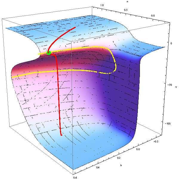
48 48 J.M. GINOUX AND J. LLIBRE FIG. 11. Numerical canards solutions and critical manifold of system (70 in the (x 1 x 3 y 1 phase space for parameter values: ε = 1/ α 2 = 0.1 β 1 = β 2 = c 1 = and c 2 =

49 CANARDS EXISTENCE IN MEMRISTOR S CIRCUITS y x FIG. 12. Numerical canardssolutions andcritical manifold ofsystem(70(x 1 y 1 phase plane for parameter values: ε = 1/ α 2 = 0.1 β 1 = β 2 = c 1 = and c 2 =

50 50 J.M. GINOUX AND J. LLIBRE 7. DISCUSSION In this work we have proposed an alternative method for determining the condition of existence of canard solutions for three and four-dimensional singularly perturbed systems with only one fast variable in the folded saddle case. This method enables to highlight a unique generic condition (σ 2 < 0 for the existence of canard solutions for such three and fourdimensional singularly perturbed systems which is based on the stability of folded singularities of the normalized slow dynamics deduced from a well-known property of linear algebra. It has been stated that this unique generic condition was perfectly identical to that provided by Benoît [6] and then by Szmolyan and Wechselberger [41] and finally by Wechselberger [47]. Finally it has been established that this condition is generic since it is exactly the same for singularly perturbed systems of dimension three and four with only one fast variable. Application of this method to the famous three and four-dimensional memristor canonical Chua s circuits for which the classical piecewise-linear characteristic curve has been replaced by a smooth cubic nonlinear function according to the least squares method has enabled to show the existence of canards solutions in such Memristor Based Chaotic Circuits. However in this paper only the case of pseudo singular points of saddletype has been analyzed. Of course the case of pseudo singular points of node-type could be also studied with the same method. Moreover this method could be successfully used for proving the existence of canard solutions in four-dimensional singularly perturbed systems with two fast variables such as the famous Hodgkin-Huxley model or in the so-called coupled FitzHugh-Nagumo system. In a future work we will state that the existence of canard solutions in such systems can be established according to the same unique generic condition (σ 2 < ACKNOWLEDGEMENTS We would like to thank to Ernesto Pérez Chavela for previous discussions related with this work. The authors are partially supported by a MINECO/FEDER grant number MTM The second author is partially supported by a MICINN/FEDER grants numbers MTM and MTM P by an AGAUR grant number 2014SGR-

51 CANARDS EXISTENCE IN MEMRISTOR S CIRCUITS by an ICREA Academia two FP7+PEOPLE+2012+IRSES numbers and and FEDER-UNAB10-4E-378.

52 52 J.M. GINOUX AND J. LLIBRE APPENDIX Change of coordinates leading to the normal forms of three and fourdimensional singularly perturbed systems with one fast variable are given in the following section. A. Normal form of 3D singularly perturbed systems with one fast variable Let s consider the three-dimensional singularly perturbed dynamical system (11 with k = 2 slow variables and m = 1 fast and let s make the following change of variables: x 1 = α 2 x x 2 = αy y 1 = αz where α << 1. (A-1 By taking into account Benoît s generic hypothesis Eqs. (2021 and while using Taylor series expansion the system (11 becomes: ẋ = f 1 y y + f 1 z z ẏ = f 2 (xyz ε α 2ż = g 1 x x+ 1 2 g 1 2 y 2 y2 + 2 g 1 y z yz g 1 2 z 2 z2. (A-2 Then let s make the standard polynomial change of variables: X = Ax+By 2 Y = y f 2 (A-3 From (A-3 we deduce that: Z = Cy +Dz. x = X Bf2 2 Y 2 A y = f 2 Y z = Z Cf 2Y D The time derivative of system (A-3 gives:. (A-4

53 CANARDS EXISTENCE IN MEMRISTOR S CIRCUITS 53 Ẋ = Aẋ+2Bvẏ Ẏ = ẏ f 2 Ż = Cẏ +Dż. (A-5 Then multiplying the third equation of (A-5 by (ε/α 2 and while replacing in (A-5 ẋ ẏ and ż by the right-hand-side of system (A-2 leads to: ( f1 Ẋ = A y y + f 1 z z +2Byf 2 Ẏ = 1 ε α 2Ż = ε ( g1 α 2Cf 2 +D x x+ 1 2 g 1 2 y 2 y2 + 2 g 1 y z yz g 1 2 z 2 z2 (A-6 Sinceε/α 2 1 the firsttermoftheright-hand-sideofthethirdequation of (A-6 can be neglected. Then replacing in (A-6 x y and z by the righthand-side of (A-4 and identifying with the following system in which we have posed: (ε/α 2 = ǫ: Ẋ = ay +bz +O ( XεY 2 YZZ 2 Ẏ = 1+O(XYZε ǫż = ( X +Z 2 +O ( εxεyεzε 2 X 2 ZZ 3 XYZ (A-7 we find: ( f1 a = A b = A D x 2 C D f 1 f 1 f 2 +2Bf2 2 y 1 (A-8 where

54 54 J.M. GINOUX AND J. LLIBRE Finally we deduce: A = 1 g 1 2 x B = g 1 z 2 [ 2 g 1 y 2 2 g 1 z 2 C = 1 2 g 1 2 y z D = 1 2 g 1 2 z 2. ( 2 2 ] g 1 y z (A-9 a = 1 2 f2 2 ( 2 g 1 x 2 2 b = g 1 x 1 f 1 2 g 1 y 2 1 ( 2 g 1 2 x ( 2 f g 1 2 g 1 f 1 2 x 1 y1 2 2 g 1 f 1 x 2 x 2 (A-10 This is the result established by Benoît [8] and presented in Sec B. Normal form of 4D singularly perturbed systems with one fast variable Let s consider the four-dimensional singularly perturbed dynamical system (30 with k = 3 slow variables and m = 1 fast and let s make the following change of variables: x 1 = α 2 x x 2 = αy x 3 = αz y 1 = αu where α 1. (A-11 By taking into account extension of Benoît s generic hypothesis Eqs. (4041 and while using Taylor series expansion the system (30 becomes: ẋ = f 1 y y + f 1 z z + f 1 u u ẏ =f 2 (xyzu ż =f 3 (xyzu ε α 2 u = g 1 x x+ 1 2 g 1 2 y 2 y g 1 2 z 2 z g 1 2 u 2 u2 + 2 g 1 y z yz + 2 g 1 y u yu+ 2 g 1 z u zu. (A-12

55 CANARDS EXISTENCE IN MEMRISTOR S CIRCUITS 55 Then let s make the standard polynomial change of variables: X = Ax+By 2 +Cz 2 Y = y f 2 Z = z f 3 +Dy (A-13 From (A-13 we deduce that: U = Ey +Fz +Gu. x = X Bf2 2 Y 2 Cf3 2(Z Df 2Y 2 A y = f 2 y z = f 3 (Z Df 2 Y u = U Ef 2Y Ff 3 (Z Df 2 Y. G The time derivative of system (A-13 gives: (A-14 Ẋ = Aẋ+2Byẏ+2Czż Ẏ = ẏ f 2 Ż = ż f 3 +Dẏ U = Eẏ +Fż +G u. (A-15 Then multiplying the fourth equation of (A-15 by (ε/α 2 and while replacing in (A-15 ẋ ẏ ż and u by the right-hand-side of system (A-12 leads to: ( f1 Ẋ =A y y + f 1 z z + f 1 u u +2Byf 2 +2Czf 3 Ẏ =1 Ż =1+Df 2 ε α U 2 = ε α 2Ef 2 + ε ( g1 α 2Ff 3 +G x x g 1 z u zu (A-16 Since ε/α 2 << 1 the two first terms of the right-hand-side of the fourth equation of (A-16 can be neglected. Then by replacing in (A-16 x y z

56 56 J.M. GINOUX AND J. LLIBRE and u by the right-hand-side of(a-14 and by identifying with the following system in which we have posed: (ε/α 2 = ǫ: Ẋ = ãy + bu +O ( XǫY 2 YUU 2 Ẏ = 1+O(XYUǫ Ż = 1+O(XYUǫ ǫż = ( X +U 2 +O ( ǫxǫyǫuǫ 2 X 2 UU 3 XYU (A-17 we find: ( f1 ã =A E x 2 G A f 1 b = G f 1 ( f1 f 2 +A F f 1 x 3 G +2Bf Cf2 3 (A-18 where A = 1 g 1 2 g 1 2 x u 2 B = f [ 3 2 g 1 2 g 1 2f 2 u 2 y z + 2 g 1 2 ] [ g g 1 2 ( g ] y u z u 4 u 2 y 2 g 1 y u [ C = 1 2 g 1 2 ( g ] 4 z 2 u 2 g 1 z u D = 1 f 2 E = 1 2 g 1 2 y u F = 1 2 g 1 2 z u G = 1 2 g 1 2 u 2. Finally we deduce: (A-19

57 CANARDS EXISTENCE IN MEMRISTOR S CIRCUITS 57 ã = 1 ( 2 g 1 2 f2 2 x ( 2 g 1 2 f2 3 x g 1 y g 1 y 2 1 ( 2 g 1 2 x 2 ( 2 g 1 x f g 1 2 x f g 1 3 x 1 ( 2 g 1 2 g 1 +f 2 f 3 x 2 x 3 y1 2 2 g 1 2 g 1 x 2 x 3 b = g 1 x 1 f 1 ( 2 g 1 y 2 1 ( 2 g 1 y 2 1 f 1 2 g 1 f 1 x 2 x 2 f 1 x 3 2 g 1 x 3 f 1 (A-20 This is the result we established in Sec Moreover let s notice that by posing f 3 = 0 in ã we find again a given in Sec Routh-Hurwitz theorem and their application to the determination of the Hopf bifurcation parameter-value in the case of three and four-dimensional singularly perturbed system are presented in this appendix. C. Routh-Hurwitz s theorem for 3D systems According to (23 the Cayley-Hamilton eigenpolynomial associated with the Jacobian of a three-dimensional singularly perturbed system(11 reads: λ 3 σ 1 λ 2 +σ 2 λ σ 3 = 0 (A-21 where σ 1 = λ 1 +λ 2 +λ 3 σ 2 = λ 1 λ 2 +λ 2 λ 3 +λ 1 λ 3 σ 3 = λ 1 λ 2 λ 3. (A-22 Let s rewrite the eigenpolynomial (A-21 as: a 3 λ 3 +a 2 λ 2 +a 1 λ+a 0 = 0 (a 0 > 0. Routh-Hurwitz theorem [39?] states that the real parts of the eigenvalues of this eigenpolynomial are negative if and only if all the following determinants: D 1 = a 1 ; D 2 = a 1 a 0 a 3 a 2 = a 1a 2 a 0 a 3 (A-23 are positive.

58 58 J.M. GINOUX AND J. LLIBRE Now let suppose that the eigenpolynomial(a-21 has one real eigenvalue λ 1 0 and two complex conjugated λ 23 = a +ıb (with a 0 an b 0. So we have: σ 1 = λ 1 +2a σ 2 = 2aλ 1 +a 2 +b 2 ( σ 3 = λ 1 a 2 +b 2. The determinant D 2 reads: (A-24 D 2 = 2a ( a 2 +b 2 +2aλ 1 +λ 2 1 (A-25 Moreover if we consider that the real part of the complex conjugated eigenvalues λ 23 depends on a parameter say µ we have a = a(µ. Then determinant D 2 vanishes at the location of the points where the real part a = a(µ. So it can be used to determine the Hopf-parameter value. D. Routh-Hurwitz s theorem for 4D systems According to (43 the Cayley-Hamilton eigenpolynomial associated with the Jacobian of a four-dimensional singularly perturbed system (30 reads: where λ 4 σ 1 λ 3 +σ 2 λ 2 σ 3 λ+σ 4 = 0 (A-26 σ 1 = λ 1 +λ 2 +λ 3 +λ 4 σ 2 = λ 1 λ 2 +λ 1 λ 3 +λ 2 λ 3 +λ 1 λ 4 +λ 2 λ 4 +λ 3 λ 4 σ 3 = λ 1 λ 2 λ 3 +λ 1 λ 2 λ 4 +λ 1 λ 3 λ 4 +λ 2 λ 3 λ 4 σ 4 = λ 1 λ 2 λ 3 λ 4. (A-27 Let s rewrite the eigenpolynomial (A-26 as: a 4 λ 4 +a 3 λ 3 +a 2 λ 2 +a 1 λ+ a 0 = 0 (a 0 > 0. Routh-Hurwitz theorem [ ] states that the real parts of the eigenvalues of this eigenpolynomial are negative if and only if all the following determinants: D 1 = a 1 ; D 2 = a 1 a 0 a 3 a 2 = a a 1 a 0 0 1a 2 a 0 a 3 ; D 3 = a 3 a 2 a 1 0 a 4 a 3 (A-28 are positive.

59 CANARDS EXISTENCE IN MEMRISTOR S CIRCUITS 59 Now let suppose that the eigenpolynomial (A-26 has two real eigenvalues λ 1 λ 2 with λ 1 λ 2 0 and two complex conjugated λ 34 = a+ıb (with a 0 an b 0. So we have: σ 1 = 2a+λ 1 +λ 2 σ 2 = a 2 +b 2 +2a(λ 1 +λ 2 +λ 1 λ 2 σ 3 = 2aλ 1 λ 2 + ( a 2 +b 2 (λ 1 +λ 2 σ 4 = ( a 2 +b 2 λ 1 λ 2. The determinant D 3 reads: (A-29 D 3 = 2a ( a 2 +b 2 +2aλ 1 +λ 2 1 (λ1 +λ 2 ( a 2 +b 2 +2aλ 2 +λ 2 2 (A-30 Moreover if we consider that the real part of the complex conjugated eigenvalues λ 23 depends on a parameter say µ we have a = a(µ. Then determinant D 3 vanishes at the location of the points where the real part a = a(µ. So it can be used to determine the Hopf-parameter value. REFERENCES 1. J. Argémi J. [1978] Approche qualitative d un problème de perturbations singulières dans R 4 in Equadiff 1978 ed. R. Conti G. Sestini G. Villari ( E. Benoît J.L. Callot F. Diener and M. Diener Chasse au canard Collectanea Mathematica (31 32 (1-3 ( E. Benoît Tunnels et entonnoirs CR. Acad. Sc. Paris 292 Série I ( E. Benoît Équations différentielles : relation entrée-sortie CR. Acad. Sc. Paris 293 Série I ( E. Benoît and C. Lobry Les canards de R 3 CR. Acad. Sc. Paris 294 Série I ( E. Benoît Systèmes lents-rapides dans R 3 et leurs canards Société Mathématique de France Astérisque ( ( E. Benoît Canards de R 3 Thèse d état (PhD Université de Nice E. Benoît Canards et enlacements Publications de l Institut des Hautes Etudes Scientifiques 72 ( E. Benoît Perturbation singulière en dimension trois : Canards en un point pseudo singulier noeud Bulletin de la Société Mathématique de France (129-1 ( J.L. Callot F. Diener and M. Diener Le problème de la chasse au canard CR. Acad. Sc. Paris 286 Série A ( L.O. Chua Memristor The Missing Circuit Element IEEE Transactions on Circuit Theory 18 (5 (

60 60 J.M. GINOUX AND J. LLIBRE 12. M. Di Ventra Y.V. Pershin and L.O. Chua Circuit elements with memory: memristors memcapacitors and meminductors Proceedings of the IEEE 97 ( M. Diener The Canard Unchained or How Fast/Slow Dynamical Systems Bifurcate Math. Intellingencer 6(3 ( N. Fenichel Persistence and smoothness of invariant manifolds for flows Ind. Univ. Math. J. 21 ( N. Fenichel Asymptotic stability with rate conditions Ind. Univ. Math. J. 23 ( N. Fenichel Asymptotic stability with rate conditions II Ind. Univ. Math. J. 26 ( N. Fenichel Geometric singular perturbation theory for ordinary differential equations J. Diff. Eq. ( A. Fitch D. Yu H. Iu and V. Sreeram Hyperchaos In A Memristor-Based Modified Canonical Chua s Circuit Int. J. of Bifurcation and Chaos 22 (6 ( A. Fitch and H. Iu Development of Memristor Based Circuits World Scientific Series on Nonlinear Science Series A 82 (World Scientific Singapore A. Fruchard and R. Schäfke Sur le retard à la bifurcation In T. Sari editor Colloque de Saint Louis (Sénégal. ARIMA 9 ( J.M. Ginoux and J. Llibre Flow curvature method applied to canard explosion Journal of Physics A: Mathematical and Theoretical 44 (46 ( J.M. Ginoux J. Llibre and L.O. Chua Canards from Chua s circuit Int. J. of Bifurcation and Chaos 23 (4 ( J.M. Ginoux and B. Rossetto The Singing Arc: The Oldest Memristor? in Chaos CNN Memristors and Beyond: A Festschrift for Leon Chua World Scientific Publishing A. Adamatsky and G. Chen (Eds. 24. J. Guckenheimer and R. Haiduc Canards at folded nodes Mosc. Math. J. 5(1 ( A. Hurwitz Über die Bedingungen unter welchen eine Gleichung nur Wurzeln mit negativen reellen Theilen besitzt Math. Ann. 41 ( M. Itoh and L.O. Chua Canards and chaos in nonlinear systems Circuits and Systems ISCAS 92. Proceedings 6 ( M. Itoh and L.O. Chua Memristors oscillators Int. J. of Bifurcation and Chaos 18 (11 ( M. Itoh and L.O. Chua Duality of Memristors Int. J. of Bifurcation and Chaos 23 (1 ( C.K.R.T. Jones Geometric Singular Perturbation Theory in Dynamical Systems Montecatini Terme L. Arnold Lecture Notes in Mathematics vol Springer- Verlag ( T. Kaper An Introduction to Geometric Methods and Dynamical Systems Theory for Singular Perturbation Problems in Analyzing multiscale phenomena using singular perturbation methods Baltimore MD ( Amer. Math. Soc. Providence RI. 31. B. Muthuswamy and P.P. Kokate Memristorbased chaotic circuits IETE Tech. Rev. 26 (

61 CANARDS EXISTENCE IN MEMRISTOR S CIRCUITS B. Muthuswamy Implementing memristor based chaotic circuits Int. J. of Bifurcation and Chaos 20 ( B. Muthuswamy and L.O. Chua Simplest chaotic circuit Int. J. of Bifurcation and Chaos 20 ( E. Nelson Internal Set Theory: a new approach to nonstandard analysis Bull. Amer. Math. Soc. 83(6 ( R.E. O Malley Introduction to Singular Perturbations Academic Press New York Y.V. Pershin and M. Di Ventra Experimental demonstration of associative memory with memristive neural networks 2009 available: L.S. Pontryagin The asymptotic behaviour of systems of differential equations with a small parameter multiplying the highest derivatives Izv. Akad. Nauk. SSSR Ser. Mat. 21(5 ( A. Robinson Nonstandard Analysis North-Holland Amsterdam E.J. Routh A Treatise on the Stability of a Given State of Motion: Particularly Steady Motion Macmillan and co D.B. Strukhov G. S. Snider G. R. Stewart and R.S. Williams The missing memristor found Nature 453 ( P. Szmolyan and M. Wechselberger Canards in R 3 J. Dif. Eqs. 177 ( F. Takens Constrained equations a study of implicit differential equations and their discontinuous solutions in Structural stability the theory of catastrophes and applications in the sciences Springer Lecture Notes in Math. 525 ( A.N. Tikhonov On the dependence of solutions of differential equations on a small parameter Mat. Sbornik N.S. 31 ( A. Tsuneda A Gallery Of Attractors From Smooth Chua s Equation Int. J. of Bifurcation and Chaos 15(1 ( B. Van der Pol On relaxation-oscillations The London Edinburgh and Dublin Philosophical Magazine and Journal of Science 7 (2 ( M. Wechselberger Existence and Bifurcation of Canards in R 3 in the case of a Folded Node SIAM J. Applied Dynamical Systems 4 ( M. Wechselberger À propos de canards Trans. Amer. Math. Soc. 364 (

62