REPORT DOCUMENTATION PAGE

Transcription

1 REPORT DOCUMENTATION PAGE Form Approved OMB NO The public reporting burden for this collection of information is estimated to average 1 hour per response, including the time for reviewing instructions, searching existing data sources, gathering and maintaining the data needed, and completing and reviewing the collection of information. Send comments regarding this burden estimate or any other aspect of this collection of information, including suggesstions for reducing this burden, to Washington Headquarters Services, Directorate for Information Operations and Reports, 1215 Jefferson Davis Highway, Suite 1204, Arlington VA, Respondents should be aware that notwithstanding any other provision of law, no person shall be subject to any oenalty for failing to comply with a collection of information if it does not display a currently valid OMB control number. PLEASE DO NOT RETURN YOUR FORM TO THE ABOVE ADDRESS. 1. REPORT DATE (DD-MM-YYYY) 2. REPORT TYPE Ph.D. Dissertation 4. TITLE AND SUBTITLE Multiscale Modeling of Advanced Materials for Damage Prediction and Structural Health Monitoring 3. DATES COVERED (From - To) - 5a. CONTRACT NUMBER W911NF b. GRANT NUMBER 6. AUTHORS Luke Borkowski 5c. PROGRAM ELEMENT NUMBER d. PROJECT NUMBER 5e. TASK NUMBER 5f. WORK UNIT NUMBER 7. PERFORMING ORGANIZATION NAMES AND ADDRESSES Arizona State University ORSPA AZ Board of Regents on behalf of Arizona State Unive Tempe, AZ SPONSORING/MONITORING AGENCY NAME(S) AND ADDRESS (ES) U.S. Army Research Office P.O. Box Research Triangle Park, NC DISTRIBUTION AVAILIBILITY STATEMENT Approved for public release; distribution is unlimited. 8. PERFORMING ORGANIZATION REPORT NUMBER 10. SPONSOR/MONITOR'S ACRONYM(S) ARO 11. SPONSOR/MONITOR'S REPORT NUMBER(S) EG SUPPLEMENTARY NOTES The views, opinions and/or findings contained in this report are those of the author(s) and should not contrued as an official Department of the Army position, policy or decision, unless so designated by other documentation. 14. ABSTRACT Advanced aerospace materials, including fiber reinforced polymer and ceramic matrix composites, are increasingly being used in critical and demanding applications, challenging the current damage prediction, detection, and quantification methodologies. Multiscale computational models offer key advantages over traditional analysis techniques and can provide the necessary capabilities for the development of a comprehensive virtual structural health monitoring (SHM) framework. Virtual SHM has the potential to drastically improve the design and analysis of aerospace components through coupling the complementary capabilities of models able to predict the initiation 15. SUBJECT TERMS composites, structural health monitoring, multiscale, damage 16. SECURITY CLASSIFICATION OF: 17. LIMITATION OF a. REPORT b. ABSTRACT c. THIS PAGE ABSTRACT UU UU UU UU 15. NUMBER OF PAGES 19a. NAME OF RESPONSIBLE PERSON Aditi Chattopadhyay 19b. TELEPHONE NUMBER Standard Form 298 (Rev 8/98) Prescribed by ANSI Std. Z39.18

2 Report Title Multiscale Modeling of Advanced Materials for Damage Prediction and Structural Health Monitoring ABSTRACT Advanced aerospace materials, including fiber reinforced polymer and ceramic matrix composites, are increasingly being used in critical and demanding applications, challenging the current damage prediction, detection, and quantification methodologies. Multiscale computational models offer key advantages over traditional analysis techniques and can provide the necessary capabilities for the development of a comprehensive virtual structural health monitoring (SHM) framework. Virtual SHM has the potential to drastically improve the design and analysis of aerospace components through coupling the complementary capabilities of models able to predict the initiation and propagation of damage under a wide range of loading and environmental scenarios, simulate interrogation methods for damage detection and quantification, and assess the health of a structure. A major component of the virtual SHM framework involves having micromechanics-based multiscale composite models that can provide the elastic, inelastic, and damage behavior of composite material systems under mechanical and thermal loading conditions and in the presence of microstructural complexity and variability. Quantification of the role geometric and architectural variability in the composite microstructure plays in the local and global composite behavior is essential to the development of appropriate scale-dependent unit cells and boundary conditions for the multiscale model. Once the composite behavior is predicted and variability effects assessed, wave-based SHM simulation models serve to provide knowledge on the probability of detection and characterization accuracy of damage present in the composite. The research presented in this dissertation provides the foundation for a comprehensive SHM framework for advanced aerospace materials. The developed models enhance the prediction of damage formation as a result of ceramic matrix composite processing, improve the understanding of the effects of architectural and geometric variability in polymer matrix composites, and provide an accurate and computational efficient modeling scheme for simulating guided wave excitation, propagation, interaction with damage, and sensing in a range of materials. The methodologies presented in this research represent substantial progress toward the development of an accurate and generalized virtual SHM framework.

3 Multiscale Modeling of Advanced Materials for Damage Prediction and Structural Health Monitoring by Luke Borkowski A Dissertation Presented in Partial Fulfillment of the Requirements for the Degree Doctor of Philosophy Approved April 2015 by the Graduate Supervisory Committee: Aditi Chattopadhyay, Chair Yongming Liu Marc Mignolet Antonia Papandreou-Suppappola John Rajadas ARIZONA STATE UNIVERSITY May 2015

4 ABSTRACT Advanced aerospace materials, including fiber reinforced polymer and ceramic matrix composites, are increasingly being used in critical and demanding applications, challenging the current damage prediction, detection, and quantification methodologies. Multiscale computational models offer key advantages over traditional analysis techniques and can provide the necessary capabilities for the development of a comprehensive virtual structural health monitoring (SHM) framework. Virtual SHM has the potential to drastically improve the design and analysis of aerospace components through coupling the complementary capabilities of models able to predict the initiation and propagation of damage under a wide range of loading and environmental scenarios, simulate interrogation methods for damage detection and quantification, and assess the health of a structure. A major component of the virtual SHM framework involves having micromechanics-based multiscale composite models that can provide the elastic, inelastic, and damage behavior of composite material systems under mechanical and thermal loading conditions and in the presence of microstructural complexity and variability. Quantification of the role geometric and architectural variability in the composite microstructure plays in the local and global composite behavior is essential to the development of appropriate scale-dependent unit cells and boundary conditions for the multiscale model. Once the composite behavior is predicted and variability effects assessed, wave-based SHM simulation models serve to provide knowledge on the probability of detection and characterization accuracy of damage present in the composite. The research presented in this dissertation provides the foundation for a comprehensive SHM framework for advanced aerospace materials. The developed i

5 models enhance the prediction of damage formation as a result of ceramic matrix composite processing, improve the understanding of the effects of architectural and geometric variability in polymer matrix composites, and provide an accurate and computational efficient modeling scheme for simulating guided wave excitation, propagation, interaction with damage, and sensing in a range of materials. The methodologies presented in this research represent substantial progress toward the development of an accurate and generalized virtual SHM framework. ii

6 To my family, especially my wife, mother, father, and sister, for their continual support, encouragement, inspiration, and patience iii

7 ACKNOWLEDGEMENTS Completion of the research presented in this dissertation was the result of efforts by many people to whom I owe much appreciation. The advice, encouragement, and challenge provided by my advisor, Regents Professor Aditi Chattopadhyay, has developed in me a passion for research and allowed me to achieve my academic goals. I am sincerely grateful for her supervision and support throughout my doctoral studies. I would also like to thank the members of my Supervisory Committee, Prof. Yongming Liu, Prof. Marc Mignolet, Prof. Antonia Papandreou-Suppappola, and Prof. John Rajadas for volunteering their time to provide valuable insight and advice in regards to my research. I greatly appreciate the guidance, mentorship, and constructive criticism I ve received throughout my studies as a PhD student from the postdoctoral researchers in Dr. Chattopadhyay s group, including Drs. Seung Bum Kim, Masoud Yekani Fard, KC Liu, and Yingtao Liu. I have also benefited greatly from collaborating and learning with my fellow graduate students and I am thankful to have developed technically and formed friendships with all of them. I would also like to thank Ms. Kay Vasley and Ms. Megan Crepeau for providing assistance with the day-to-day tasks of the AIMS Center. The research presented in this dissertation was supported in part by the National Science Foundation Graduate Research Fellowship Program under Grant No ; Army Research Office under Grant No EG, Program Manager Dr. Asher Rubinstein; Air Force Office of Scientific Research MURI Program under Grant No. FA , Technical Monitor Dr. David Stargel; and in collaboration with Aerojet Rocketdyne. iv

8 TABLE OF CONTENTS Page LIST OF TABLES... x LIST OF FIGURES... xi CHAPTER 1 INTRODUCTION Motivation and Background Objectives of the Work Outline of the Dissertation MULTISCALE MODEL OF WOVEN CERAMIC MATRIC COMPOSITES CONSIDERING MANUFACTURING INDUCED DAMAGE Introduction Multiscale Generalized Method of Cells Overview MSGMC Microscale Governing Equations MSGMC Mesoscale Governing Equations MSGMC Macroscale Governing Equations Extension of MSGMC to Predict Manufacturing Induced CMC Damage Modeling Woven CMCs using MSGMC Void and Interphase Modeling Constitutive Relations and Damage Model v

9 CHAPTER Page Physical Model Architectural and Mechanical Properties Results and Discussion Conclusion THE EFFECT OF MICROSTRUCTURE ON COMPOSITE MECHANICAL PERFORMANCE Introduction Micromechanics Modeling of Unidirectional Composite Fiber Variability Development of 3D RUC Finite Element Model Rate Dependent Inelasticity Consideration Generation and Quantification of Microstructural Variability Results and Discussion Global Elastic Composite Behavior Local Inelastic Composite Behavior Experimental versus Simulated Microstructures Conclusion FULLY COUPLED ELECTROMECHANICAL ELASTODYNAMIC MODEL FOR GUIDED WAVE PROPAGATION ANALYSIS Introduction vi

10 CHAPTER Page 4.2 Three-Dimensional Electromechanical Coupled Elastodynamic Model Framework Governing Equations and Discretization Enforcement of Elastodynamic Equilibrium and Continuity of Traction Final Expressions for Nodal Mechanical Displacement Enforcement of Maxwell s Equation and Continuity of Electric Displacement Final Expressions for Nodal Electrical Potential Simulation Results and Discussion Physical Model Development Theoretical Validation Computational Efficiency Collocated Actuators for Selective Lamb Wave Mode Suppression Effect of Actuation Type Relationship between Piezoelectric Sensor Displacement and Output Voltage Imposing Stress-Free Boundary Conditions Conclusion vii

11 CHAPTER Page 5 ELETRO-MAGNETO-MECHANICAL ELASTODYNAMIC MODEL FOR LAMB WAVE DAMAGE QUANTIFICATION IN COMPOSITES Introduction Three-Dimensional Electro-Magneto-Mechanical Coupled Elastodynamic Model Framework Governing Equations and Discretization Enforcement of Elastodynamic Equilibrium and Continuity of Traction Final Expressions for Nodal Mechanical Displacement Enforcement of Maxwell s Equation (Gauss s Electric Field Law) and Continuity of Electric Displacement Final Expressions for Nodal Electrical Potential Enforcement of Maxwell s Equation (Gauss s Magnetic Field Law) and Continuity of Magnetic Flux Density Final Expressions for Nodal Magnetic Potential Simulation and Experimental Results and Discussion Experimental Setup and Physical Model Development Experimental Validation Computational Efficiency Lamb Wave Propagation in a Laminated Composite Plate viii

12 CHAPTER Page Damage Detection Capabilities of the Developed Model Conclusion CONTRIBUTIONS AND FUTURE WORK Contributions Future Work REFERENCES ix

13 LIST OF TABLES Table Page 2.1. C/SiC Weave Architecture Properties Plain Weave C/SiC Tow Architecture Properties Constituent Temperature-Independent Material Properties Fiber Properties (Bowles and Tompkins, 1989) Matrix Properties (Bowles and Tompkins, 1989) Prediction of Global Composite CTE Constituent Material Properties Material Parameters for Viscoplasticity Model PZT (APC 850) Orthotropic Properties Computational Efficiency Comparison between FEM and Current Model Comparison of Simulated Wave Speeds using Different Actuation Types for fb/2 Equal to 300 khz-mm CFRP Composite Plate Laminae Properties Piezomagnetic Material (CoFe2O4) Properties Computational Efficiency Comparison between FEM and Current Model x

14 LIST OF FIGURES Figure Page 2.1. Concurrent Multiscale Model Analysis Framework MSGMC Unit Cells Illustrating the Analysis of a Multiscale Material at Various Length Scales and with Arbitrary Coordinate Systems (Aboudi, Arnold, and Bednarcyk, 2012) Micro-/mesoscale RUC of High and Low Fidelity Fiber with Voids Contained in Matrix Subcells Composite Subcell Stacks Plain Weave RUC with Localized Void Structure Carbon Fiber CTE vs. Temperature (Pradere and Sauder, 2008) Matrix CTE vs. Temperature (Dow Chemical Company, 2013) RUCs Employed at the Micro- and Mesoscales to Account for Matrix Void Architectural Variability PyC CTE vs. Temperature (Luo and Cheng, 2004) Matrix Tensile Modulus vs. Temperature (Dow Chemical Company, 2013) Nonlinear Tensile Behavior of Plain Weave C/SiC Residual von Mises Stress (GPa) and Damage State Progression in 2D Fiber/Matrix Subcell RUC during Cool-Down from 1023 o C to 23 o C Damage State Progression in 2D Fiber/Matrix Subcell RUC during Cool-Down from 1023 o C to 23 o C Effect of Matrix Voids on Damage Progression during Cool-Down in Unidirectional C/SiC Composite xi

15 Figure Page Effect of Matrix Voids on Tensile Modulus Reduction during Cool-Down in Unidirectional C/SiC Composite Effect of Matrix Voids on In-Plane Shear Modulus Reduction during Cool- Down in Unidirectional C/SiC Composite Damage Variable Progression and Reduction in Tensile Modulus for Plain Weave C/SiC Composite during Cool-Down Damage State Variable Progression during Cool-Down for Two Subcell Stacks within the Plain Weave RUC Damage Initiation and Progression as a Function of Position within Plain Weave RUC Matrix and Undulation Subcell Stack Illustration Tow Subcell Stack Illustration Expanded Views of Damage Initiation and Final State as a Function of Position within the Plain Weave RUC Micrograph of PMC at 1000X Magnification Meshed FEM Microstructural Model Mesh Convergence Analysis Representation of Reference Node Positions Kinematic Periodicity in RUC Simulated Microstructures Generated using a Monte Carlo Perturbation Framework Ripley s K-Function for Three Simulated Microstructures xii

16 Figure Page 3.8. Two-Point Correlation (S11) Function for Three Simulated Microstructures Microstructure Statistical Convergence Demonstrated using Plots of the Two- Point Correlation Function Probability Density Functions for Experimental Micrograph Fiber Diameter Measurements Global Elastic Moduli vs. Microstructural Randomness for Composite RUC Containing Constant Fiber Radii Volume Averaged Stress Ratio vs. Microstructural Randomness von Mises Stress Contour (GPa) of Unidirectional Composite Loaded in Transverse Tension von Mises Stress Contour (GPa) of Unidirectional Composite Loaded in Transverse Shear Global Elastic Moduli vs. Microstructural Randomness for Composite RUC Containing Experimentally Determined Distribution of Fiber Radii von Mises Stress Contour (GPa) of Unidirectional Composite with Random Distribution of Fiber Radii Loaded in Transverse Tension von Mises Stress Contour (GPa) of Unidirectional Composite with Random Distribution of Fiber Radii Loaded in Transverse Shear Global Tensile Moduli (E11 and E22) vs. Microstructural Randomness for Composite RUC Effective Inelastic Strain Contour for Ordered RUC Effective Inelastic Strain Contour for Hard-Core RUC xiii

17 Figure Page Maximum Effective Inelastic Strain at Four Strain Rates for an Ordered Microstructure Maximum Effective Inelastic Strain at Four Strain Rates for a Semi-Random Microstructure Maximum Effective Inelastic Strain at Four Strain Rates for a Hard-Core Microstructure Cauchy Stress vs. Applied Global Strain from Three Microstructures Loaded at 1E-3/s Strain Rate Cauchy Stress vs. Applied Global Strain for Hard-Core Distribution at Four Strain Rates Microstructures for Statistical Equivalence Verification Experimental vs. Simulated Microstructure K-Functions Statistical and Mechanical Equivalence of Two Simulated Microstructures Relative Tensile Modulus vs. Microstructural Order (Experimental to Hard- Core) Definition of Nodal Points and Supplemental LISA/SIM Grid Points Simulated Plate Geometry (Not to Scale) Cycle Cosine Tone Burst Excitation Theoretical Validation of A0 and S0 Lamb Wave Mode Group Velocities Relative Actuator Voltage Poling Directions and Resultant Through-Thickness Displacement Profile (Out-of-Plane) for Collocated Piezoelectric Actuation for Selective Lamb Wave Mode Suppression xiv

18 Figure Page 4.6. Through-Thickness Plots of (a) Out-of-Plane Displacement, (b) In-Plane Displacement, and (c) Vector Field for A0 Lamb Wave Mode at t= µs for fb/2=300 khz-mm Through-Thickness Plots of (a) Out-of-Plane Displacement, (b) In-Plane Displacement, and (c) Vector Field for S0 Lamb Wave Mode at t= µs for fb/2=300 khz-mm Through-Thickness Plots of (a) Out-of-Plane Displacement, (b) In-Plane Displacement, and (c) Vector Field for A0 Lamb Wave Mode at t=33.25 µs for fb/2=300 khz-mm Through-Thickness Plots of (a) Out-of-Plane Displacement, (b) In-Plane Displacement, and (c) Vector Field for S0 Lamb Wave Mode at t=33.25 µs for fb/2=300 khz-mm Comparison of Sensor Voltage between Symmetric and Antisymmetric Zeroth Order Lamb Wave Modes for fb/2 Equal to (a) 200 khz-mm, (b) 300 khz-mm, (c) 400 khz-mm, and (d) 500 khz-mm Excitation of GW in Plate using Three Different Actuation Types: (a) Displacement in the Y-Direction, (b) Displacement in the Z-Direction, and (c) Voltage Actuation Sensor Signal Comparison for Three Different Actuation Types for fb/2 Equal to 300 khz-mm Comparison of Sensor Voltage and Nodal Displacement Components Beneath Sensor for fb/2 Equal to 300 khz-mm xv

19 Figure Page Vacuum and Air Cells Surrounding Plate used to Impose Stress-Free Boundary Conditions Convergence of Mean Sensor Signal using Three Different Kinds of Boundary Cells Sensor Signal Comparison for Three Different Boundary Cells for fb/2 Equal to 500 khz-mm Composite Dispersion Curve Experimental Validation Setup Simulated and Experimental Dispersion Curve Comparison for Range of Frequency-Thickness Products Commonly Used for Damage Detection in Composites Through-Thickness Plots of (a) In-Plane Displacement, (b) Out-of-Plane Displacement, and (c) Vector Field for A0 Lamb Wave Mode at t=45.60 µs for fb/2=525 khz-mm Through-Thickness Plots of (a) In-Plane Displacement, (b) Out-of-Plane Displacement, and (c) Vector Field for S0 Lamb Wave Mode at t=45.60 µs for fb/2=525 khz-mm Flash Thermography Images of Low Velocity Impact Induced Localized Delamination and Distributed Matrix Cracking / Fiber Breakage (Hiche et al., 2009) Illustration of Simulated Damage (i.e., Matrix Cracking) Surrounding Delamination xvi

20 Figure Page 5.7. Sensor Voltage vs. Time Signature Demonstrating the Phase Shift and Amplitude Change as a Result of Delamination and Damage Relative ToF and Peak Amplitude for Three Fundamental GW Modes in Composite Plate with fb/2=525 khz-mm for Varying Delamination and Damage Sizes Relative ToF and Peak Amplitude for A0 Lamb Wave Mode in Composite Plate with fb/2=525 khz-mm for Varying Delamination and Damage (Matrix Cracking) Sizes xvii

21 1 INTRODUCTION 1.1 Motivation and Background The constituent and architectural complexity, multiscale characteristics of damage, and anisotropic scattering and dispersion of elastic waves in advanced aerospace materials has made investigations of damage prediction, detection, and life estimation a critical factor for ensuring structural reliability and safety. To date, a comprehensive understanding of the performance of aerospace composites under critical loading and environmental conditions is still lacking, and the full potential of these material systems has yet to be exploited (Ghosh, Lee, and Raghavan, 2001). Physics-based computational models play a key role in predicting damage initiation and propagation as a result of mechanical and thermal loading conditions, simulating the interaction of elastic and electromagnetic waves with the predicted damage, and assessing the current condition of the structure. Because of the complexities associated with aerospace materials, in particular fiber-reinforced composites, damage prediction and quantification studies are often limited to two-dimensional (2D) geometries, linearly elastic constitutive models, prescribed damage initiation location and progression path, and ordered microstructures (Murthy and Chamis, 1986; Freund, 1990; Sankar and Marrey, 1997; Lee and Staszewski, 2003; Swaminathan, Ghosh, and Pagano, 2006; Skoček, Zeman, and Šejnoha, 2008). These assumptions can lead to oversimplification of the problem, and therefore, often result in poor prediction of the critical behavior of these materials. On the other hand, virtual structural health monitoring (SHM) methodologies have been shown to enhance the capabilities of stand-alone damage prediction and SHM systems and to 1

22 improve damage detection and characterization capabilities in structures comprising advanced aerospace materials (Chattopadhyay et al., 2009). Current SHM techniques, although capable of interrogating large structures, are often insensitive to small-scale damage, which limits their successful implementation when the tolerant damage size in a structure is below that which can be detected using SHM methods. Because of this inherent limitation of wave-based SHM techniques, physicsbased multiscale damage prediction models can serve as a valuable tool to provide prior knowledge for maximizing the probability of early detection. Traditional analysis techniques based on plate lamination theory or homogenized linear elastic tow and ply properties have proven to be inadequate for capturing the multiscale damage prevalent in advanced aerospace materials, especially fiber-reinforced composites with braided or woven architectures (Reddy, 2004). Multiscale modeling techniques, on the other hand, have demonstrated the capacity to provide the necessary physical considerations, robustness, and geometric and architectural fidelity for predicting elastic, inelastic, and damage behavior across all applicable length and time scales (Aboudi, 2013). Additionally, these techniques allow the scale-dependent field variables of composites (e.g., stress, strain, damage) to be propagated across relevant length scales using appropriate bridging methods. This, in turn, allows prediction of the local and global behavior of the composite as a function of parameters at the micro-, meso-, and macroscales, in addition to investigation of its effect at the scale(s) of interest. Micromechanics-based multiscale models provide a valuable tool for evaluating the full range of behavior (e.g., elastic, inelastic, nonlinear, damage) of a wide array of material systems (e.g., woven polymer and ceramic matrix composites, cross-ply 2

23 composites, and aerospace metal alloys). Using this technique, damage initiation and failure in individual constituents of composites can be modeled explicitly through the development and application of advanced constitutive relations at the microscale. Homogenization, which accounts for the degraded load carrying capacity of the microscale repeating unit cell (RUC) as well as any relevant scale-dependent variability, provides the upper length scales with necessary information related to damage, inelasticity, and nonlinearity. The coalescence of microscale damage is manifested as tow splitting, matrix/tow debonding, and intertow matrix cracking at the mesoscale. At the macroscale, the lower length scale damage contributes to ply failure, delamination, and structural degradation. Efficiency, maintained by only transferring necessary information across the scales, is crucial to the effectiveness of the multiscale framework to contribute statistically significant damage information to the SHM models for a range of loading scenarios, boundary conditions, and microstructural variability. The importance of accurate and efficient multiscale damage prediction as an integral component of a virtual SHM framework stems from the need for prior knowledge on damage size, location, type, and severity so a proper assessment of the probability of detection and quantification can be made by SHM experiments and models. The presence of damage at multiple length scales induces changes in the local and global behavior of aerospace composites caused by variation in elastic moduli, density, conductivity (e.g., electrical, thermal), magnetic permeability, and residual stresses. The spatial variations in mechanical, electrical, and thermal properties are compounded by geometric and architectural variability present in the microstructure of the composite. Traditionally, nondestructive evaluation (NDE) methods have been utilized to detect and 3

24 quantify manufacturing defects and in-service damage (Adams and Cawley, 1988). However, major advancements in sensor technology, data management, signal processing, electronic packaging, and prognosis has allowed conventional NDE techniques to be extended to in-situ real-time environments to provide online damage assessment capabilities. This extension of NDE is often referred to as SHM and has the capability to vastly enhance damage detection, localization, quantification, prognosis, as well as the prediction of residual useful life (RUL) in aerospace materials, which will in turn improve safety and reduce the cost of maintaining current and future airframes (Farrar and Worden, 2007; Mohanty, Chattopadhyay, and Peralta, 2010). Wave-based damage detection and quantification techniques have been demonstrated as an effective and economical means of structural interrogation (Su, Ye, and Lu, 2006; Raghavan and Cesnik, 2007; Giurgiutiu, 2008); however, extension of the simulation methods used to model these techniques is necessary for the consideration of all the relevant physics involved and to provide a generalized framework that is not limited to a small set of materials, geometries, or damage events. Both accuracy and computational efficiency are necessary for a wave propagation modeling scheme to serve as an effective tool in providing knowledge regarding the physics of the problem for the purpose of improving experimental wave-based SHM frameworks for aerospace structures. Because of the complex nature of ultrasonic wave excitation, propagation, and interaction with material features and damage at various length scales, computation tools are necessary to investigate the mechanisms responsible for wave dispersion, attenuation, scattering, and coupling. Modeling ultrasonic wave excitation and sensing is crucial to wave propagation simulation techniques because of the complex coupling between the electrical and/or 4

25 magnetic excitation of the piezoelectric and/or piezomagnetic actuators, the subsequent mechanical response of the actuator and structure, and finally the mechanical, electrical, and/or magnetic response of the sensor. Limited resources prohibit the experimental characterization and testing of every conceivable damage scenario under all potential loading and environmental conditions using a range of NDE and SHM techniques; therefore there is an urgent need to develop multiscale damage models coupled with appropriate virtual SHM methodologies to provide relevant data for estimating damage initiation and propagation, probability of detection, and RUL of aerospace components. In this dissertation, a virtual SHM framework is developed that includes the following: i) a physics-based multiscale damage prediction model of a woven ceramic matrix composite (CMC) accounting for damage formation as a result of the manufacturing process as well as void distribution and size, ii) a micromechanics-based model to investigate the effect of architectural and geometric variability on the local and global elastic and inelastic behavior of laminated composites, and iii) a wave propagation model capable of efficiently simulating the behavior of elastic waves in anisotropic media, their excitation and sensing, and their interaction with damage, geometric features, and material property spatial variation. These models contribute to the overarching goal of developing a comprehensive virtual SHM framework that is capable of capturing and simulating damage initiation, detection, and characterization in the presence of material geometric and architectural variability and complexity. Due to the robustness and generality of the proposed modeling scheme, various actuation signals, frequencies, and wave types (e.g., bulk, guided, surface) can be considered to determine the optimal ultrasonic features, characterization methods, and transducer locations for a 5

26 wide range of damage scenarios, material constituent properties, and microscale architectures. In addition to accurately capturing the physics of the problem, emphasis is placed on maintaining computational efficiency for both the damage prediction and detection models to ensure the developed framework remains feasible for use in virtual SHM. Multiscale models play an important role in capturing the nonlinear response of woven carbon fiber reinforced CMCs. In plain weave carbon fiber/silicon carbide (C/SiC) composites, for example, when microcracks form in the as-produced parts due to the mismatch in thermal properties between constituents, a multiscale thermoelastic framework can be used to capture the as-received damage state of these composites. In this research, a micromechanics-based multiscale model coupled with a thermoelastic progressive damage constitutive law is developed to simulate the elastic and damage behavior of a plain weave C/SiC composite system under thermal and mechanical loading conditions (Borkowski and Chattopadhyay, 2013; Borkowski and Chattopadhyay, 2015). The multiscale model is able to accurately predict composite behavior and serves as a valuable tool in investigating the physics of damage initiation and progression, in addition to the evolution of effective composite elastic moduli caused by temperature change and damage. The matrix damage initiation and progression is investigated at various length scales and the effects are demonstrated on the global composite behavior. Microstructural variation in advanced aerospace materials, such as fiber-reinforced composites, has a direct relationship with its local and global mechanical performance. When micromechanical modeling techniques for unidirectional composites assume a uniform and periodic arrangement of fibers, the bounds and validity of this assumption 6

27 must be quantified. One goal of this research is to characterize the influence of microstructural randomness on effective homogeneous response and local inelastic behavior (Borkowski, Liu, and Chattopadhyay, 2013b; Borkowski, Liu, and Chattopadhyay, 2014). The knowledge gained from this work provides insight into when the microscale architectural uncertainty should be considered for a multiscale model in order to be able to accurately capture the homogenized global behavior and localized inelastic response of a fiber-reinforced composite. The results indicate that for a carbon fiber reinforced polymer matrix unidirectional composite system, microstructural progression from ordered to disordered decreases the tensile modulus by 5%, increases the shear modulus by 10%, and substantially increases the magnitude of local inelastic fields (Borkowski, Liu, and Chattopadhyay, 2013b; Borkowski, Liu, and Chattopadhyay, 2014). The experimental and numerical analyses presented in this work demonstrate the importance of microstructural variability when lower length scale phenomena drive global response. In the study of wave propagation for SHM and the development of improved damage detection methodologies, physics-based computational models play an important role. Due to the complex nature of guided wave (GW) propagation, accurate and efficient computational tools are necessary to investigate the mechanisms responsible for dispersion, coupling, and interaction with damage. In this work, a fully coupled electromagneto-mechanical elastodynamic model for wave propagation in heterogeneous, anisotropic material systems is developed (Borkowski, Liu, and Chattopadhyay, 2013a; Borkowski and Chattopadhyay, 2014). The final framework provides the full threedimensional (3D) displacement as well as magnetic and electrical potential fields for 7

28 arbitrary plate and transducer geometries and excitation waveform and frequency. The model is validated theoretically for an aluminum specimen and experimentally for a cross-ply composite specimen and proven to be computationally efficient. Studies are performed with surface bonded piezoelectric transducers as well as embedded piezomagnetic transducers to gain insight into the physics of experimental techniques used for SHM. Collocated actuation of the fundamental Lamb wave modes is modeled over a range of frequencies to demonstrate mode tuning capabilities. The effect of delamination and damage (i.e., matrix cracking) on the GW propagation is demonstrated and quantified. Since many NDE and SHM studies, including the ones investigated in this work, are time and resource intensive and often difficult to perform experimentally, the developed model provides a valuable tool for the improvement and expansion of current SHM techniques. 1.2 Objectives of the Work The overarching goal of the research presented in this dissertation is to develop and extend the necessary building blocks for a virtual SHM framework that will combine traditional multiscale damage prediction and multiphysics damage detection simulation tools to enhance the capabilities and feasibility of advanced SHM platforms and systems. The following are the principal objectives of this work: 1. Develop a multiscale physics-based model incorporating thermomechanical constitutive relations and a continuum damage mechanics based progressive damage law to capture the initiation and propagation of matrix damage in a woven CMC material system under thermomechanical loading and environmental conditions. 8

29 2. Investigate the effect of microstructural spatial variation on local and global elastic and inelastic fields in fiber-reinforced composites. Determine when the explicit consideration of experimental random microstructures is necessary and when the assumption of ordered arrays provides sufficiently accurate results. 3. Develop an accurate and efficient wave propagation model to investigate the physics of wave-based SHM techniques for the detection, localization, and quantification of damage in advanced aerospace materials. 4. Incorporate electromechanical coupling into the elastodynamic modeling scheme, previously proven effective in simulating wave propagation in the presence of material discontinuities, to allow accurate simulation of GW actuation and sensing using piezoelectric transducers. 5. Extend the elastodynamic wave propagation model to include piezomagnetic and electromagnetic coupling to expand the actuation and sensing modeling capabilities of the framework. 6. Demonstrate the effectiveness of the developed damage prediction and quantification models in serving as a virtual SHM framework to investigate numerous loading, environmental, and geometric scenarios. 1.3 Outline of the Dissertation The dissertation is structured as follows: Chapter 2 presents the development of a multiscale model to simulate the processing effects, in addition to mechanical loading, on the damage behavior of CMCs utilized in aerospace applications. Focus is placed on capturing the thermoelastic behavior and progressive damage as a function of environmental conditions, temperature-dependent 9

30 material properties, and architectural features. A key consideration of the presented modeling scheme is the use of scale-specific RUCs that permit the relevant architectural features at each scale, such as voids, to be modeled. Chapter 3 focuses on the development of a finite element method (FEM) based micromechanics model to investigate the effect of fiber position variation on the transverse behavior of a unidirectional composite material system. Elastic and inelastic constitutive behavior and rate-dependent effects of the polymer matrix constituent are investigated. A major focus of this study is to determine how local and global fields vary as a function of microstructural variation, including global elastic properties and local damage initiation and progression. Chapter 4 introduces the development and validation of an electromechanical coupled wave propagation model for the simulation of GWs in an arbitrary material system, actuated and sensed using piezoelectric transducers. The model is validated theoretically and used to investigate the physics of Lamb wave excitation, propagation, and sensing. The novel solution of electromechanically coupled governing equations using a methodology commonly used for GW modeling addresses a major deficiency in the framework. Additionally, the improved computational efficiency and accuracy over a model solved using a commercial FEM software is demonstrated. Chapter 5 introduces an extension of the work presented in Chapter 4. In addition to electromechanical coupling, the governing equations are re-derived to include magnetomechanical and electromagnetic coupling. This additional coupling permits the modeling of a wider array of NDE and SHM actuation and sensing methods including piezomagnetic and Eddy current. Guided wave propagation is demonstrated in a cross-ply 10

31 laminated carbon fiber reinforced composite and validated experimentally. The effect of delamination and dispersed damage (e.g., matrix microcracking and fiber breakage) on the Lamb wave propagation is investigated. Further improvements in the computational efficiency are also presented. Chapter 6 summarizes the research work reported in this dissertation and emphasizes the important original contributions and findings of this dissertation. Suggestions on future research directions and recommendations are also discussed at the end of this chapter. 11

32 2 MULTISCALE MODEL OF WOVEN CERAMIC MATRIC COMPOSITES CONSIDERING MANUFACTURING INDUCED DAMAGE 2.1 Introduction The extreme stiffness, strength, and toughness, as well as nonbrittle failure of advanced CMCs make them an ideal choice over traditional materials for many aerospace applications, such as for components used in the hot section of turbine engines, rocket nozzles, and thermal protection systems (Inghels and Lamon, 1991; Camus, Guillaumat, and Baste, 1996; El Bouazzaoui, Baste, and Camus, 1996; Jacobsen and Brøndsted, 2001; Murthy, Gyekenyesi, and Mital, 2004; Aboudi, 2011; Goldberg, 2012; Goldsmith et al., 2014). Additionally, CMCs offer oxidation and creep resistance and thermal shock stability at elevated temperatures. However, under extreme loading and environmental conditions, the structural reliability of these composites remains a critical issue because a damage event will compromise the integrity of the composite structure, resulting in ultimate failure. Damage in CMCs can initiate at the fiber, matrix, tow, or weave level. The widespread use of CMCs in critical aerospace components such as turbine blades and thermal barriers, therefore, necessitates development of physics-based models that can accurately account for constitutive linear elastic and nonlinear behavior at the pertinent length scales of these materials. Multiscale models can link constitutive model parameters and behavior at the micro- and mesoscale to elastic behavior and damage evolution at the macroscale, thus further extending our understanding of damage initiation and propagation in heterogeneous material systems. Traditional analysis methods for composites account for only macroscopic or structural level responses, rendering them inadequate in capturing the complex multiscale phenomena governing 12

33 composite behavior. Multiscale physics-based models, on the other hand, are well-suited for high fidelity structural analysis because they can effectively determine stress, strain, stiffness, damage, and various other state variables at multiple length scales; in fact, some multiscale techniques, such as the Multiscale Generalized Method of Cells (MSGMC), are capable of analyzing the relevant scales of the composite concurrently (Paley and Aboudi, 1992). These models also enable simultaneous information transfer between scales using appropriate localization and homogenization techniques Multiscale Generalized Method of Cells Overview In this chapter, a recently developed multiscale modeling technique is further extended to incorporate manufacturing-related, temperature-dependent damage behavior as a function of thermal and mechanical loading and nonuniform void distribution in CMCs. MSGMC, developed by Liu et al. (2011a) extends the Generalized Method of Cells (GMC) theory (Paley and Aboudi, 1992; Aboudi, 1995) to include additional length scales beyond the micro- and global scales, thereby allowing for the analysis of woven or braided composite architectures. Hence, the number of length scales under investigation is not limited by the analysis technique, but rather can be determined by the physically relevant length scale dependent phenomena that must be captured in the analysis. For example, in the case of a woven composite, as shown in Figure 2.1, the relevant length scales may include: (i) constituent level (microscale), (ii) tow level (mesoscale), (iii) weave level (macroscale), and (iv) structural level. Figure 2.1 also demonstrates the relevant features at each length scale taken into consideration in the multiscale analysis, including the void structure within the inter- and intratow matrix. 13

34 Figure 2.1. Concurrent Multiscale Model Analysis Framework The fundamental equations and framework of the MSGMC theory are provided in this chapter for clarity. For the detailed derivation of the theory, the reader is directed to Liu et al. (2011a) and Aboudi, Arnold, and Bednarcyk (2012). The extension of GMC to include the consideration of an arbitrary number of length scales (as is the case for MSGMC) is possible because of the recursive nature of the developed framework where the GMC unit cell can either be composed of a monolithic material or an additional GMC unit cell, as seen in Figure 2.2. This additional GMC unit cell can also either be composed of monolithic material subcells or another GMC unit cell to be analyzed at a lower length scale. The successive analysis of lower length scale unit cells occurs until all unit cells contain only monolithic material; it is at this scale that the elastic, inelastic, and thermal constitutive and damage models are applied. Therefore, this framework is well-suited for modeling the multiscale behavior of woven or braided composites where the various 14

35 geometric and architecturally relevant scales (i.e., micro-, meso-, and macroscales as seen in Figure 2.1) can be represented appropriately. The analysis of woven or braided composites begins with the spatial discretization of the triply periodic macroscale unit cell (i.e., weave level) into Nα, Nβ, N subcells comprising either intertow matrix or fiber tow bundles (i.e., tows), as seen in Figure 2.2. The tow subcells are then further discretized into a doubly periodic unit cell with Nβ, N subcells where the constituent (e.g., fiber, intratow matrix, interphase material) constitutive behavior is applied. In this summary of the MSGMC governing equations at each length scale, the quantity of superscript indicial sets for each field variable (e.g., { }{ } [] αβ β ), where each set of indices is contained in curly brackets and the closed brackets represent an arbitrary field variable, provides an indication of the length scale at which the variable exists while the indices within the set indicate the periodicity of the unit cells at each length scale. For example, the field variable { }{ } [] αβ β exists two scales below the macroscale (i.e., microscale) and the unit cell at that scale is a doubly periodic RUC (e.g., { β }) and is contained within a triply periodic RUC (e.g., { αβ }). 15

36 Figure 2.2. MSGMC Unit Cells Illustrating the Analysis of a Multiscale Material at Various Length Scales and with Arbitrary Coordinate Systems (Aboudi, Arnold, and Bednarcyk, 2012) MSGMC Microscale Governing Equations The constitutive behavior of the composite constituents is applied at the microscale, and the higher length scale behavior (e.g., stress state, tangent moduli) is achieved through the successive homogenization of the lower length scales using the GMC theory (Paley and Aboudi, 1992; Aboudi, 1995). The stresses at the microscale (denoted by superscript { αβ }{ β }) are computed using Equation (2.1). { αβ }{ β} { αβ }{ β} { αβ }{ β} I{ αβ }{ β} σ = C ε ε (2.1) where { αβ }{ β} { }{ } αβ β C is the constituent stiffness matrix, ε is the total microscale strain { }{ } I αβ β tensor in the subcell determine via localization from the mesoscale, and ε is the inelastic micro-strain computed using the applied inelastic constitutive model, if applicable. Strains are localized from higher length scales, as seen in Equation (2.2), 16

37 using the total and inelastic strain concentration matrices, { αβ }{ β } A and { αβ}{ β} D, respectively, which are functions of the subcell geometry and stiffness matrix. { αβ }{ β } { αβ }{ β } { αβ } { αβ }{ β } I{ αβ } ε = A ε + D ε (2.2) The overbar indicates average quantities of the unit cell or subcell as a function of lower I{ } αβ length scale parameters and ε represents a tensor containing all the subcell inelastic strains in the unit cell { αβ } MSGMC Mesoscale Governing Equations s The mesoscale response of the composite at the fiber tow/intertow matrix length scale is governed by the microscale response as well as mesoscale geometric parameters such as fiber packing arrangement and tow volume fraction. A mesoscale RUC is shown in Figure 2.3 where the fiber, matrix, interphase, and void constituents shown in black, red, gray, and black and white hatched, respectively, are modeled at the microscale and their cumulative response contributes to that of the mesoscale. Homogenization of the microscale stresses provides the mesoscale unit cell stresses, s { αβ } σ, as seen in Equation (2.3). The mesoscale stress tensor can also be represented by an effective constitutive law, Equation (2.4), where the equation for the effective stiffness tensor, provided in Equation (2.5). { αβ } C, is 17

38 Figure 2.3. Micro-/mesoscale RUC of High and Low Fidelity Fiber with Voids Contained in Matrix Subcells N{ αβ } β N{ αβ } 1 σ σ (2.3) { αβ} { αβ }{ β} σ h{ } l αβ β { αβ } h{ } l αβ { αβ } { αβ } β = 1{ αβ} = 1 = { αβ } { αβ } { αβ } I{ αβ } σ = C ε ε (2.4) where N{ αβ} β N{ αβ} 1 C C Α (2.5) { αβ} { αβ}{ β} { αβ}{ β} h{ } l αβ β { αβ} h{ } l αβ { αβ } { αβ} β = 1{ αβ} = 1 = The homogenization of the microscale inelastic strain tensor to achieve an expression for the mesoscale inelastic strain tensor ( ε I{ αβ } ) is provided by 18

39 ε { αβ} I N{ αβ} { αβ} = 1 { αβ } C = h l 1 N{ αβ } β { αβ} { αβ} { αβ} β { αβ } β { αβ} = 1 ( D ε s ε ) { αβ}{ β} { αβ }{ β } I{ αβ} I{ αβ}{ β} h l C (2.6) while the effective total strain tensor, as and { αβ } ε, localized from the macroscale, is expressed { αβ } { αβ } { β } { αβ } I{ β } ε = A ε + D ε (2.7) tt tt s where I I{ } { } { } 11 I NβN ε s = ε,..., ε, { β} { β} { β} I ε = A ε + D ε (2.8) I s ip ip s { ε,..., ε } { β } I{ 1β} I{ Nα β } ε =, and ε is the globally applied strain. The subscripts ip and tt on the strain concentration matrices A and D indicate the in-plane and through-thickness portion of the two-step homogenization procedure outlined in Chapter MSGMC Macroscale Governing Equations The composite macroscale response is governed by the cumulative effects of the micro- and mesoscale behavior as well as macroscale geometric and architectural parameters such as overall volume fraction, tow geometry, and lamina thickness. The composite subcell stacks that are utilized to assemble the macroscale RUC are shown in Figure 2.4 and comprise weft, warp, overlapping, and matrix subcell stacks. Each of the subcells in the stacks is analyze at either the microscale or mesoscale depending on if it contains monolithic matrix or a fiber tow. Simulation of a range of composite woven architectures is possible through varying the arrangements of subcell stacks. Once 19

40 assembled, a two-step homogenization process is utilized to achieve the stiffness and stress of the periodic macroscale unit cell. This process, developed by Bednarcyk (2000) and Bednarcyk and Arnold (2003), is employed to overcome the lack of shear coupling inherent in the GMC formulation. The equations comprising the through-thickness and in-plane homogenization processes are shown in Equations (2.9) through (2.11) and Equation (2.12) through (2.14), respectively. Through-thickness homogenization Figure 2.4. Composite Subcell Stacks { } 1 N α β { αβ } σ = σ dα (2.9) d α = 1 { } 1 N α β { αβ } { αβ } C = Αtt C dα (2.10) d α = 1 1 { β } Nα { β} C { αβ } { αβ } { β } { αβ } = dαc Dtt s d α = 1 ( ) I I I ε ε ε (2.11) ε ε ε 20

41 In-plane homogenization 1 N β N { β} σ hβl hl β = σ σ (2.12) = 1 = 1 1 N β N { β} { β } ip hβl hl β C A C (2.13) = = 1 = 1 ( ip s ) 1 Nβ N I C ε =- hβlc D ε ε hl β = 1 = 1 { β} { β} I I{ β} ε ε ε (2.14) Combining the constitutive relations and homogenization and localization expressions from the micro-, meso-, and macroscales, it is possible to obtain expressions linking field quantities across all the relevant length scales. Therefore an expression for the microscale stresses can be achieved as a function of the globally applied macroscale strain as well as the relevant concentration matrices as seen in Equation (2.15). ( { } { } ( + ) + { αβ }{ β} { αβ }{ β} { αβ }{ β } { αβ } { β} { β} I αβ I β σ =C A A tt Aip ε Dip ε s Dtt ε s (2.15) { αβ }{ β} I{ αβ } I{ αβ }{ β} +D ε s ) ε Inversely, the homogenized macroscale stress and stiffness matrix can be expressed as functions of the lower length scale stress, stiffness, and geometric and architectural parameters as seen in Equations (2.16) and (2.17), respectively. N N{ } N β N { } 1 Nα 1 αβ β αβ d α { αβ }{ β } σ = h l β h{ } l{ } αβ β αβ hl β 1 1 d σ (2.16) = = α = 1 h{ } l αβ { αβ } { αβ } β = 1 { αβ } = 1 and 21

42 1 C = hl 1 d Nα Nβ N β = 1 = 1 A { β} ip { αβ } Att d h l α h l β N{ αβ} β N{ αβ} α { αβ} { αβ} { αβ} β { αβ} = 1 = 1 = 1 C { αβ }{ β} { αβ }{ β } A h{ } l αβ β { αβ} (2.17) Extension of MSGMC to Predict Manufacturing Induced CMC Damage The MSGMC framework used in this work has previously been demonstrated effective for predicting the linear elastic and nonlinear inelastic and damage behavior of different types of composites (e.g., polymer matrix composites (PMCs) and CMCs with woven and braided architectures) in a highly computationally efficient manner (Liu et al., 2011a; Liu and Arnold, 2011; Liu and Arnold, 2013). This framework is further extended to include the following important manufacturing related phenomena in CMCs: (i) thermal residual stress and damage state following manufacturing; (ii) interaction between nonuniform void distributions and stress and damage fields; and (iii) global nonlinear behavior due to multiscale damage and release of thermal residual stresses. The material system analyzed in this research is a plain weave C/SiC composite. The triply periodic plain weave RUC analyzed using the MSGMC framework is assumed to be representative of the entire periodic composite structure. For the analysis, the weave is discretized into several sub-volume cells, as seen in Error! Reference source not ound.. In this figure, the through-thickness discretization utilized by MSGMC to represent the woven tow architecture is evident; the four cells in the thickness direction are composed of either matrix subcells (red) or tow subcells (white with black lines representing tow fiber direction). The specific CMC under investigation is manufactured through densification of the carbon fiber preform via a chemical vapor infiltration (CVI) 22

43 process, which follows the coating of the carbon fibers with a pyrolytic carbon (PyC) interphase, also performed via CVI (Jacobsen and Brøndsted, 2001). Since the carbon fibers are susceptible to corrosion at elevated temperatures, the PyC interphase offers increased corrosion resistance while also serving as a toughening mechanism through crack deflection, fiber/matrix debonding, and fiber pullout (Lamouroux et al., 1993). Due to the manufacturing process and insufficient infiltration (i.e., canning) of the matrix material, voids are distributed in the composite nonuniformly (Sullivan et al., 2006). Using the MSGMC multiscale modeling scheme, the effects of void distribution, volume fraction, and shape on the nonlinear damage-driven macroscopic CMC response were previously investigated in a deterministic and stochastic framework by Liu and Arnold (2011) and Liu and Arnold (2013), respectively. It was concluded that void geometric and architectural parameters, especially shape and localization, greatly influence the elastic and damage characteristics of a CMC. The nonuniform shape and size of voids in the composite microstructure is therefore considered in the analyses presented in this chapter and described in further detail in the Chapter Figure 2.5. Plain Weave RUC with Localized Void Structure 23

44 The innovative aspect of this research lies in the inclusion of manufacturing process effects within the multiscale analysis on the as-produced state and nonlinear mechanical behavior of the composite under mechanical and thermal loading conditions and in the presence of nonuniform and multiscale void structure. The CVI process, which is typically isothermal and isobaric and carried out at a temperature between 900 o C and 1100 o C (Mei et al., 2007), is examined. As the specimen cools to room temperature following CVI, the mismatch in the temperature-dependent coefficients of thermal expansion (CTEs) between the carbon fiber and silicon carbide matrix, as presented in Figure 2.6 and Figure 2.7, respectively, causes thermal residual stresses to develop in the composite. Specifically, large residual stresses develop between the plies of the laminated composite and at the fiber/matrix interface during the cool-down phase following manufacturing. The residual stresses, in turn, cause microcracks to form in the inter- and intratow matrix. Because of the heterogeneity and complex architecture of the woven composite material system, the manufacturing-induced damage is distributed nonuniformly within the composite. Accounting for the presence, distribution, and severity of such damage in the as-produced state of the composite is critical for predicting the as-received mechanical properties, further damage evolution and progression, and subsequent failure in CMC structural components. This research contributes to the core focus of the Integrated Computational Materials Engineering (ICME) approach, which aims to integrate the length and time scales, processing/manufacturing conditions, structural and architectural information, and constituent behavior of materials into a comprehensive, multiscale modeling scheme for the purpose of improving material design and optimization (Panchal, Kalidindi, and McDowell, 2013). 24

45 Figure 2.6. Carbon Fiber CTE vs. Temperature (Pradere and Sauder, 2008) Figure 2.7. Matrix CTE vs. Temperature (Dow Chemical Company, 2013) In woven CMCs manufactured through the CVI process, the complex damage behavior is due in part to tow undulation and crossing, porous intratow matrix, and large intertow voids (Inghels and Lamon, 1991; Aubard, Lamon, and Allix, 1994; Peters, Martin, and Pluvinage, 1995; Kuo and Chou, 1995). Addressing this problem with a 25

46 multiscale framework allows for the damage to be captured at the most relevant length scale (i.e., matrix constituent level). Additionally, a continuum damage mechanics based progressive damage model is developed, and damage evolution is tracked across the length scales using state variables. The progressive damage approach allows subcells to continue carrying load even after the initiation of damage, as opposed to other approaches that utilize maximum stress/strain or failure laws (Murthy, Gyekenyesi, and Mital, 2004; Goldberg, 2012). Following initiation, the subsequent evolution of damage in the subcell is controlled by a progressive damage law. In addition, the presence of nonuniform void shape and size affects the global moduli and damage behavior of the composite. The presence of severe matrix microcracking in the as-produced C/SiC composite (Sullivan et al., 2006) results in the material system exhibiting nonlinearity in its mechanical behavior, even at very low stress levels. Therefore, in addition to stimulating thermally induced damage, the multiscale model developed in this chapter will also be able to predict the nonlinear behavior of the composite when subsequent mechanical loading is applied. 2.2 Modeling Woven CMCs using MSGMC Void and Interphase Modeling In CMCs manufactured via the CVI process, the concentration of voids in the weave tends to be nonuniform due to insufficient and uneven infiltration of the matrix material into the carbon fiber preform (Sullivan et al., 2006). Optical micrographs, such as those presented in Sullivan et al. (2006) and Murthy, Gyekenyesi, and Mital (2004) demonstrate the variation in void shape, size, and distribution as a function of location within the composite. Typically, the intertow matrix surrounding the regions in which a 26

47 tow is undulating has a higher volume fraction of voids compared with those away from the regions of undulation. Additionally, these voids tend to be sheet-like in form. Therefore, the model accounts for this variation in intertow matrix void distribution, size, and shape as a mesoscale input parameter. Voids also exist within the intratow matrix cells and micrographs indicate that these voids are evenly dispersed and uniform in size (Camus, Guillaumat, and Baste, 1996; El Bouazzaoui, Baste, and Camus, 1996; Murthy, Gyekenyesi, and Mital, 2004; Sullivan et al., 2006). The meso- and microscale voids are accounted for at a length scale below that at which the matrix constituent (either at the meso- or microscale) is examined by analyzing a separate RUC and homogenizing the properties to provide higher length scale effective properties (Liu and Arnold, 2011). The purpose of analyzing a separate RUC for the void subcells is twofold: (i) to dampen the effects the voids have on the stiffness reduction of the row and column in which the void resides within the RUC and (ii) to represent the voids in a more accurate and generalized framework. In GMC theory, because of the constant strain field assumption for each subcell, a subcell with an approximate zero stiffness (e.g., a void subcell) will cause the entire row and column in which it resides within the RUC to be eliminated due to homogenization (Aboudi, Arnold, and Bednarcyk, 2012). The fiber tow bundles are modeled as 4x4 doubly periodic RUCs, as presented in Figure 2.8 (a), consisting of a fiber cell (black), the surrounding interphase material cells (shaded), and the intratow matrix cells (red). The intra- and intertow voids are accounted for by modeling the micro- and mesoscale matrix cells containing the voids as 2x2x2 subcells consisting of one cube-like void cell (white) and seven matrix subcells (red) as seen Figure 2.8 (b) and as 4x1 subcells consisting of one sheet-like void cell (white) and 27

48 three matrix subcells (red) as seen Figure 2.8 (c), respectively. The size of the void cell is a function of the void volume fraction. The scale at which the subcells containing voids is modeled (meso- or microscale) depends on the location of the matrix subcell (within or between fiber tow bundles). Modeling the voids and fiber interphase as described provides a generalized framework in which to model the meso- and microscale architecture and material properties of a CMC composite while capturing the effect of voids on the composite behavior as a result of stress concentrations, reduction in effective elastic properties, and damage initiation and propagation. (a) 4x4 Fiber Tow Bundle RUC (b) 2x2x2 Intratow Matrix and Void RUC (c) 4x1 Intertow Matrix and Void RUC Figure 2.8. RUCs Employed at the Micro- and Mesoscales to Account for Matrix Void Architectural Variability Constitutive Relations and Damage Model Due to the nature of CMCs (e.g., high void content, weak fiber/matrix bonding, quasibrittle matrix), multiscale models have the potential to play a key role in predicting the initiation and progression of damage at the most relevant scale, while propagating this information, using homogenization and localization approaches, to the length scales of greatest interest. Liu and Arnold (2011) have developed a damage mechanics based progressive damage model for the ceramic constituent material in CMCs. This damage 28

49 model is extended to also include thermal coupling and temperature-dependent material properties and model parameters. Matrix damage initiation and propagation in the model is represented by a scalar damage mechanics constitutive model, which is driven by the magnitude of the hydrostatic stress and strain tensor. Damage criteria based on the magnitude of the hydrostatic tensors have previously been utilized successfully to represent the damage behavior of quasi-brittle matrix material systems (Mazars, 1986; Resende, 1987; Lemaitre and Desmorat, 2005). Aboudi (2011) utilized the anisotropic damage law proposed by Lemaitre and Desmorat (2005) and coupled it with the High Fidelity Generalized Method of Cells (HFGMC) micromechanics framework to predict the damage evolution in ductile and quasi-brittle matrix composites. Wu, Li, and Faria (2006) demonstrated that for composite systems with quasi-brittle matrices loaded in tension, fracture is predominately activated by tensile damage mechanisms in both the deviatoric and volumetric stress spaces. In other words, mode I fracture is the dominant failure mode in these systems (Resende, 1987; Wu, Li, and Faria, 2006). Damage initiation and progression in the developed model is governed by a bilinear constitutive relation for the elastic/damageable matrix subcells where the model parameters n and σcrit represent the damage normalized secant modulus and the critical stress at which damage initiates, respectively. The application of the damage law at the microscale matrix constituent level permits the use of such a model since the dilation at the material point will serve to separate the material particles, thereby initiating a matrix microcrack. The material properties (e.g., K 0 ), model parameters (e.g., n and σcrit), and stress and strain are assumed to be functions of temperature to allow for the consideration of thermal effects on the composite constitutive and damage behavior. Although the 29

50 present damage law is isotropic at the matrix subcell level, the aggregate effect of damage in each individual subcell on the behavior at the higher length scales can be highly anisotropic, depending on the loading and boundary conditions imposed. The CMC matrix constituent, silicon carbide, is modeled as a homogeneous, isotropic material with temperature-dependent properties subjected to the proposed scalar progressive damage law. The equivalent stress and strain in the matrix material, denoted by subscript eq, are functions of the undamaged temperature-dependent material bulk modulus and CTE (i.e., K 0 and α 0, respectively) and the relative change in temperature, T. Damage initiates in the material subcell once the equivalent stress reaches a critical value for the particular material (σcrit). As seen in Equation (2.18), the critical equivalent stress can be a function of strain rate and temperature. 0 0 (, T, K, ) (, T ) σ ε α σ & ε (2.18) eq eq crit Once the critical stress value in a matrix cell is exceeded, a scalar damage parameter, φ, is activated that accounts for the progressive microcracking that occurs in the matrix as a result of thermal and mechanical loading. The damage variable φ scales the elastic stiffness tensor and ranges from zero (i.e., undamaged) to one (i.e., complete loss of load carrying capacity). The multiscale micromechanics-based modeling framework allows the progressive damage to be accounted for with a scalar quantity since the composite is modeled at the individual constituent level, therefore capturing the damage at the most relevant length scale. Additionally, the damage scalar at the constituent level can be homogenized and propagated up the length scales as a state variable, providing the effect of the microscale damage at each length scale considered in the analysis. The scalar 30

51 damage parameter is incorporated into the matrix temperature-dependent constitutive relation yielding a thermoelastic damage constitutive relation, as seen in Equation (2.19). In Equation (2.19), the elastic strain ( ε e ) is expressed as the total strain (ε) minus the t thermal strain ( ε = α T) using classical additive decomposition of strain. Accounting for the thermal strains in this analysis permits consideration of the damage and mechanical effect on the composite caused by the CTE mismatch between the constituent materials. ( 1 φ ) C ( T ) ( 1 φ ) e σ = ε α = C ε (2.19) where σ is the second-order Cauchy stress tensor and Cis the fourth-order linear elastic stiffness tensor. A damage rule based on the theory of elasticity in differential form is defined, as in Equation (2.20), where the equivalent stress and strain are defined as the hydrostatic stress and strain, respectively, to govern the magnitude/progression of damage: f = nk T δε δσ = (2.20) 0 e 3 ( ) eq eq 0 where n represents the damaged normalized secant modulus; K 0 is the undamaged tangent bulk modulus as a function of temperature; and 0 0 ( ( ) ( ) ) eq = eq T T T T (2.21) e δε δε δα α δ provides the elastic portion of the increment in the strain tensor where δε is the eq increment in the total equivalent strain tensor, and 0 e δσeq 3 K( λ, K ) δεeq =, (2.22) where λ= ( 1 φ ). The damage rule can be expressed in incremental form as 31

52 f = nk T δε δσ =, (2.23) 0 n+ 1 e, n+ 1 n+ 1 3 ( ) eq eq 0 where n 1 T + is the temperature at the next increment and e, n+ 1 δε eq and δσ + n 1 eq are the increments in elastic strain and stress tensors, respectively. n In order to derive an expression for δσ + 1 eq in terms of the temperature-dependent undamaged bulk modulus, the expressions for n 1 σ + eq n and σ eq are expressed as ( K T ) ( ) 0 n 0 n+ 1 n n+ 1 ( α ( T ) δα ( T ))( T δ T ) σ = 3 n K ( T ) + δ ( ) ε + δε n+ 1 0 n 0 n+ 1 n n+ 1 eq eq eq + + (2.24) and n 0 n n 0 n n σeq = 3 nk ( T ) εeq α ( T ) T. (2.25) By subtracting Equation (2.25) from (2.24) and ignoring higher order terms, the expression for the increment in equivalent stress is obtained as a function of the undamaged bulk modulus, as seen in Equation (2.26). { δσ = 3 n K ( T ) δε α ( T ) δ T δα ( T ) T n+ 1 0 n n+ 1 0 n n+ 1 0 n+ 1 n eq eq + δk ( T ) ε α ( T ) T 0 n+ 1 n 0 n n eq } (2.26) Expanding the second term in the damage law as a function of the instantaneous bulk modulus requires casting the increment in stress in terms of strain as follows: σ = 3 ε + δε ( ) 0 n 0 n+ 1 n n+ 1 ( α ( T ) δα ( T ))( T δ T ) n+ 1 n n+ 1 eq eq eq ( eq ) Subtracting Equation (2.28) from Equation (2.27) results in 32, (2.27) n n n n n σ = 3 K ε α ( T ) T. (2.28) eq

53 ( eq ) ( eq ( ) ) δσ = 3 K δε α ( T ) δ T δα ( T ) T n+ 1 n n+ 1 0 n n+ 1 0 n+ 1 n eq + δk ε α T T n n n n (2.29) where the instantaneous bulk modulus at the current and next increment, n K and n 1 K +, respectively, are expressed in terms of the original, undamaged bulk modulus, the current damage scalar, and the increment in the damage scalar as seen in Equation (2.30) and Equation (2.31), recalling that λ= ( 1 φ ). K = λ K 0 ( T ) (2.30) n n n ( λ δλ )( ( ) δ ( )) n + 1 n n n 0 n + 1 K = + K T + K T (2.31) The increment in the instantaneous bulk modulus is obtained through subtraction of Equation (2.30) from Equation (2.31), resulting in the following expression after ignoring all higher order terms. n+ 1 n 0 n+ 1 n+ 1 0 n δk = λ δk ( T ) + δλ K ( T ) (2.32) After substituting the derived expressions for the terms in the damage rule, the following expression is obtained. f = n δk ( T ) ε δk ( T ) α ( T ) T + K ( T ) δε 0 n+ 1 n 0 n+ 1 0 n n 0 n n+ 1 eq eq K ( T ) ( T ) T K ( T ) ( T ) T 0 n 0 n n+ 1 0 n 0 n+ 1 n α δ δα + 1 ( δεeq 0 α ( ) δ δα ( ) ) 1 ( eq 0 ( ) ) 0 K T T T T n n n n n n δk ε α T T n+ n n n + = (2.33) Following simplification and collection of like terms, solving for the increment in one minus the damage scalar (i.e., δλ + n 1 ) yields the formulation for the incremental, temperature-dependent, thermoelastic progressive damage law. 33

54 δλ n+ 1 ( { n+ n n n ( eq ) ( δεeq α δ δα ) ( eq ) δ ε α n K ( T ) ( T ) T + K ( T ) ( T ) T ( T ) T 0 n n 1 0 n n 1 0 n 1 n λ K ( T ) δε α ( T ) δ T δα ( T ) T n 0 n n 1 0 n n 1 0 n 1 n ( eq )}) 0 n+ 1 n 0 n n + δk ( T ) ε α ( T ) T = K ( T ) ( T ) T ( εeq α ) 0 n n 0 n n (2.34) The T300 carbon fibers of the plain weave preform used as reinforcement in the CMC material system under investigation behave linear elastically and fail under the Hashin failure criterion (Hashin, 1980; Blackketter, Walrath, and Hansen, 1993). This criterion applied within the multiscale framework determines the catastrophic/brittle failure of each individual carbon fiber and is based on the axial and shear strengths of the fiber material, as seen in Equation (2.35). Once the failure criterion exceeds a value of unity, the stiffness of the fiber is reduced to zero, thus redistributing the load away from the failed fiber and to the surrounding fibers and matrix. The compliant PyC interphase applied to the fibers during the CVI manufacturing process is assumed to fail with the fiber and does not contribute to the transverse failure modes because of its relatively low stiffness h = σ ( σ13 σ12 ) σ + + (2.35) axial τaxial Physical Model Architectural and Mechanical Properties The weave and tow architectural properties for the composite material system under investigation are presented in Table 2.1 and Table 2.2, respectively. The T300 carbon fibers are modeled as transversely isotropic and the CVI-SiC and CVI-PyC as isotropic materials. The elastic properties of the T300 carbon fiber and PyC interphase materials do 34

55 not vary significantly with temperature and therefore were assumed constant as seen in Table 2.3. However, the CTEs for these two materials were considered as functions of temperature. The temperature-dependent axial and transverse CTEs for the carbon fiber from Pradere and Sauder (2008) are presented in Figure 2.6. Luo and Cheng (2004) provided the tabular CTE data for the PyC interphase material, as seen plotted in Figure 2.9. The isotropic CTE and tensile modulus for the CVI-SiC (Figure 2.7 and Figure 2.10, respectively) were adapted from Dow Chemical Company (2013). The spatial variation of temperature-dependent properties due to architectural and constituent variability causes the development of thermal strains, which in turn contribute to the microcracks and residual stresses present in the as-produced composite. Table 2.1. C/SiC Weave Architecture Properties Type Plain Total Fiber Volume Fraction 43% Total Void Volume Fraction 15.3% Weave Void Volume Fraction 10%, 80% Total Thickness 6.55 mm Matrix CVI-SiC Interphase PyC 35

56 Table 2.2. Plain Weave C/SiC Tow Architecture Properties Tow Fiber Volume Fraction 56% Tow Void Volume Fraction 3% Tow Packing Structure Square Fiber T300 Carbon Matrix CVI-SiC Interphase PyC Table 2.3. Constituent Temperature-Independent Material Properties Constituent T300 CVI-PyC E11 (GPa) E22 (GPa) G12 (GPa) ν ν

57 Figure 2.9. PyC CTE vs. Temperature (Luo and Cheng, 2004) Figure Matrix Tensile Modulus vs. Temperature (Dow Chemical Company, 2013) 2.3 Results and Discussion The thermal constitutive model and homogenization of the constituent level CTEs to the macroscale using the MSGMC framework utilized in this chapter was validated by simulating the global longitudinal and transverse CTE of a unidirectional PMC (T300/934) with a 57% fiber volume fraction and a CMC (HMS/Borosilicate) with a fiber volume fraction of 47%, and comparing these results to those obtained using a highfidelity FEM model from Bowles and Tompkins (1989). The transversely isotropic fiber 37

58 and isotropic matrix constituent material properties for the two validation models are presented in Table 2.4 and Table 2.5, respectively. The prediction of the thermal behavior of the two composite material systems, presented in Table 2.6, was within ~5% of the FEM results. Therefore it is evident that the multiscale model is able to accurately capture the thermal linear elastic behavior of fiber-reinforced material system as a function of its constituent thermal properties. Table 2.4. Fiber Properties (Bowles and Tompkins, 1989) (10-6 / o C) E11 E22 G12 G23 Fiber (GPa) (GPa) (GPa) (GPa) ν12 ν23 α1 α2 T HMS Table 2.5. Matrix Properties (Bowles and Tompkins, 1989) Matrix E (GPa) G (GPa) ν α (10-6 / o C) 934 epoxy Borosilicate glass

59 Table 2.6. Prediction of Global Composite CTE T300/934 (PMC) Present Model FEM αl 0.084e-6/ o F 0.089e-6/ o F αt 16.56e-6/ o F 16.53e-6/ o F HMS/Borosilicate (CMC) Present Model FEM αl -0.18e-6/ o F e-6/ o F αt 2.59e-6/ o F 2.46e-6/ o F Once the thermal linear elastic composite behavior was validated, the plain weave carbon fiber reinforced CMC detailed in Table 2.1, Table 2.2, and Table 2.3 was used to validate the developed thermoelastic constitutive relation with progressive matrix damage for thermal and mechanical loading. Damage model parameter values of 180 MPa and 0.04 were used for the critical stress (σcrit) and the damage normalized secant modulus (n), respectively (Liu and Arnold, 2011). The composite was subjected to a two-part loading scheme that involved a globally stress-free cool-down from the manufacturing temperature of ~1000 o C to room temperature, followed by the loading of the specimen in uniaxial tension. During cool-down, the temperature was incremented by 1 o C for a total temperature change of 1000 o C to ensure convergence. It is assumed that the slow rate of passive cooling following the CVI process does not induce significant thermal gradients; therefore isothermal conditions were applied to the model. Due to a mismatch in CTE between the fiber and matrix materials, damage occurred during the cool-down phase, thereby introducing microcracks that reduce the initial modulus of the as-produced composite and leave the composite in a prestressed state. Following cool-down, loading 39

60 the specimen in tension caused the damage to progress further, contributing to the nonlinear tensile behavior of the C/SiC composite. The results from the simulation were plotted with the experimental results from Jacobsen and Brøndsted (2001), as seen in Figure To determine if the as-produced mechanical state of the composite was accurately predicted, the initial tensile modulus was compared to experimental data from Jacobsen and Brøndsted (2001) and Shuler et al. (1993). The initial tensile modulus is taken as the slope of the uniaxial tensile stress/strain curve before yielding or further damage occurs (i.e., first kink in the stress/strain response). The initial tensile modulus obtained from the thermoelastic simulation was ~107.5 GPa. Experimental moduli of ~113.5 and ~100.0 GPa were obtained by Jacobsen and Brøndsted (2001) and Shuler et al. (1993), respectively. A subsequent simulation was performed to determine the error that would result if the damage induced during the thermal cool-down of the plain weave CMC was ignored. An initial tensile modulus of GPa was predicted for the pristine specimen (i.e., without matrix microcracking), resulting in an overprediction of the asproduced stiffness of the specimen by approximately 35%. 40

61 Figure Nonlinear Tensile Behavior of Plain Weave C/SiC Once it was verified that the developed model could accurately predict the asproduced mechanical properties and nonlinear response of a plain weave C/SiC composite, various studies were conducted to investigate in greater detail the damage progression and development of residual stresses. The first study involved modeling a high-fidelity circular fiber using MSGMC representing a unidirectional composite RUC or a microscale RUC in a woven composite. Stress-free boundary conditions were imposed, and the RUC was subjected to thermal loading (1000 o C reduction in temperature). The matrix behavior was governed by the developed thermoelastic constitutive damage relation, and the fiber was assumed to behave linear elastically. The carbon fiber and silicon carbide matrix material properties were allowed to vary with temperature. Figure 2.12 demonstrates the cool-down phase where the mismatch in constituent CTE causes damage initiation and progression due to the development of residual stresses. Each contour in Figure 2.12 represents the damage state or stress state of the 2D RUC with a 10% void volume fraction at 200 o C increments over the 1000 o C 41

62 range. One can recall that the damage variable, λ, begins with a value of one (no damage) and decreases in value, representing the reduction in the load carrying capacity of the matrix material subcell, until it reaches zero. It can be observed that the development of residual stress surrounding the fiber correlates well with the progression of damage. As one would expect, damage initiates first in the cells nearest to the fiber/matrix interface, then progresses outward into the surrounding matrix subcells. Therefore, the degree of damage in a matrix subcell is inversely proportional to its distance from the fiber/matrix interface. 42

63 (a) Residual von Mises Stress (GPa) Contour 43 (b) Damage State Variable (λ) Contour Figure Residual von Mises Stress (GPa) and Damage State Progression in 2D Fiber/Matrix Subcell RUC during Cool- Down from 1023 o C to 23 o C

64 A subsequent study was conducted using a 2D RUC with a high-fidelity circular fiber at the center to investigate the effect of voids on the damage behavior of the ceramic constituent in C/SiC CMCs. The cool-down thermal loading process was simulated for two cases: (i) silicon carbide matrix without voids and (ii) silicon carbide matrix with a 10% volume fraction of intratow voids. Although the tow matrix material of CMCs manufactured using the CVI process will always contain at least a small volume fraction of voids, depending on the manufacturing conditions such as infiltration rate and time, the volume fraction of voids in these composites can vary significantly. Therefore, this study can provide insight into the variation in damage propagation between composites manufactured under conditions that result in varying degrees of porosity. In Figure 2.13, damage state variable contours are presented for the two cases. The interphase material was omitted from the contours in Figure 2.12 and Figure 2.13 because it does not significantly contribute to the progressive damage and its presence does not affect the trend in progression of stress and damage within the RUC. Since the progressive damage model is only applied to the matrix material, the damage value/color of the fiber in Figure 2.13 remains constant at a value of unity. It can be observed from the contours that damage for the two cases initiates at different temperatures and progresses at varying rates. For example, the contour of the final damage state for the matrix without voids (Figure 2.13 (a)) shows the presence of greater damage than that of the second case (Figure 2.13 (b)). 44

65 (a) Damage State Variable (λ) Contour for Matrix without Voids 45 (b) Damage State Variable (λ) Contour for Matrix with Voids (10% Volume Fraction) Figure Damage State Progression in 2D Fiber/Matrix Subcell RUC during Cool-Down from 1023 o C to 23 o C

66 Since it is difficult to gain a quantitative understanding of the damage initiation and progression from the damage variable contours presented in Figure 2.13, the multiscale model is called upon to bridge the scales and provide the composite response at the higher length scales. The phenomenon of matrix damage as a function of porosity is more clearly demonstrated through homogenization of the damage variable over the entire RUC volume to provide an effective damage state of the RUC, as shown in Figure This homogenization, carried out through volume-weighted averaging, is purely for qualitative purposes; the effect of the constituent level progressive damage (i.e., reduction in subcell stiffness) on the higher length scales is accounted for through homogenization of the effective stiffness matrix based on GMC theory (Aboudi, Arnold, and Bednarcyk, 2012). Interestingly, damage initiates earlier in the cool-down process (i.e., at a higher temperature) for the case with matrix voids; however, once the damage initiates in the RUC without matrix voids, the rate of damage is higher and the final reduction in load carrying capacity is greater (i.e., more significant damage). It is hypothesized that the earlier initiation of damage in the matrix with voids is caused by the stress concentration effect of the voids whereas the rapid progression of damage in the matrix without voids is a result of higher concentration of matrix material facilitating more efficient and rapid load transfer between neighboring matrix subcells. Figure 2.15 and Figure 2.16 provide insight into the evolution of elastic moduli (in-plane transverse tensile and shear moduli, respectively) as a result of damage over the same range of temperatures. The effect of microscale voids on the initial effective composite tensile and shear moduli can be observed as well as the variation in the reduction of elastic moduli due to matrix damage as a function of temperature. 46

67 Figure Effect of Matrix Voids on Damage Progression during Cool-Down in Unidirectional C/SiC Composite Figure Effect of Matrix Voids on Tensile Modulus Reduction during Cool-Down in Unidirectional C/SiC Composite 47

68 Figure Effect of Matrix Voids on In-Plane Shear Modulus Reduction during Cool- Down in Unidirectional C/SiC Composite Moving up the length scales in the multiscale model, the thermoelastic damage behavior of a 2D plain weave C/SiC composite, simulated using a 3D triply periodic RUC, was investigated during the cool-down phase following the CVI process. By overlaying the plots of the effective damage and tensile modulus versus temperature, as seen in Figure 2.17, it can be observed that the progression of the in-plane tensile modulus, E22, follows that of the damage variable, λ. Recall from Figure 2.10 that the elastic moduli of the matrix material increases with a decrease in temperature. Similarly, the effective in-plane modulus of the plain weave composite increases until damage initiates between 700 o C and 600 o C. The undamaged elastic modulus of the matrix material continues to increase as the temperature decreases; however, the increase in the value of the damage variable serves to reduce/scale the effective moduli, thereby contributing to the nonlinear behavior. Comparing Figure 2.15 and Figure 2.17, the evolution of the tensile modulus for the plain weave is seen to be more complex. This is 48

69 due to the increased architectural complexity of the fiber preform at the macroscale and fiber tow bundles at the mesoscale, which causes greater heterogeneity in damage and redistribution of stress. Figure Damage Variable Progression and Reduction in Tensile Modulus for Plain Weave C/SiC Composite during Cool-Down While the homogenized response (elastic and damage) of the 3D RUC during manufacturing and mechanical loading provides insight into the global composite behavior, further investigation can be conducted to obtain information regarding the localized damage behavior in the 3D weave architecture. Therefore, using the developed multiscale thermoelastic damage framework, the spatial effect within the discretized RUC on damage was determined at various length scales. A simulation of the manufacturing process for a plain weave C/SiC composite was conducted and the damage as a function of position within various matrix subcells of the RUC presented, as seen in Figure 2.18 and Figure Figure 2.18 presents a plot of the damage state variable versus temperature for two matrix subcell stacks. The two subcell stacks, as illustrated in 49

70 Figure 2.20, are composed of matrix cells at the mesoscale. Within these matrix subcells, the intertow void content and structure are considered. The Matrix Subcell Stack in Figure 2.20 represents a matrix-rich location in the woven RUC caused by the separation of parallel weft and warp fiber tow bundles, while the Undulation Subcell Stack indicates a location at which the undulation of the fiber tow bundle causes high matrix concentration above and below the tow. Through examination of Figure 2.18, the difference between the initiation and final state of damage within the two subcells is evident. Damage initiates at a higher temperature and evolves to a greater extent in the homogenized matrix subcell stack as compared with the undulation subcell. This result initially seems counterintuitive since one would expect the presence of fibers in the undulation subcell to cause greater damage as a result of the CTE mismatch. However, after closer inspection of the discretized RUC in Figure 2.20, it can be seen that the matrix subcell stack is in contact with fiber subcells (undulating and overlapping) on four sides in addition to at each corner, as compared to just three sides for the undulating subcell. The increased contact with neighboring fiber tow subcells promotes greater damage within the matrix cells. 50

71 Figure Damage State Variable Progression during Cool-Down for Two Subcell Stacks within the Plain Weave RUC Figure Damage Initiation and Progression as a Function of Position within Plain Weave RUC 51

72 Figure Matrix and Undulation Subcell Stack Illustration Progressing down the length scales to the microscale, the damage initiation and evolution as a function of position within fiber/matrix subcells is investigated and presented in Figure The damage behavior is examined at two locations within the microscale RUC (near the fiber (NF) and away from the fiber (AF)) for two throughthickness substacks (undulating tow (UT) and overlapping tow (OT)). Illustrations of the through-thickness substacks are presented in Figure 2.21, while the microscale RUC used for this analysis is similar to those presented in Figure From Figure 2.19, it is evident that variation in the initiation, progression, and final state of damage exists as a function of RUC location. Therefore, expanded views of the plots at the damage initiation and final temperatures are presented in Figure 2.22 (a) and (b), respectively. Damage is observed initiating at a higher temperature in the cool-down process for the undulating tow cells in comparison with the overlapping tow cells. The damage progresses at similar rates for the two subcell locations while a difference of approximately 8% is present in their final damage states. The earlier initiation and more severe final state of damage for the undulating tows are likely caused by the boundary conditions imposed on the 52

73 undulating tow by the matrix subcells surrounding it. In other words, the contraction of the matrix subcells will be less than that of the fibers within the undulating tow subcells, therefore subjecting the matrix within the undulating subcells to greater tensile loading. It can also be seen that damage initiates earlier (i.e., at a higher temperature) in matrix subcells near the fiber (NF) compared with those away from the fiber (AF) for both tow subcells investigated. This is in agreement with the results presented in Figure 2.12 and Figure As the temperature progresses to room temperature, the damage state variables for the subcell locations near the fiber and away from the fiber appear to converge, indicating damage saturation within the microscale RUC. Figure Tow Subcell Stack Illustration 53

74 (a) Damage Initiation (b) Final Damage State Figure Expanded Views of Damage Initiation and Final State as a Function of Position within the Plain Weave RUC 2.4 Conclusion A thermoelastic constitutive damage model was developed and implemented into a multiscale modeling framework to account for the manufacturing-induced residual stresses and strains and resulting matrix microcracking in carbon fiber reinforced CMCs. Capturing the as-produced state of the material system requires consideration of the manufacturing stage following the CVI process. As the composite cools during this stage, microcracks form in the matrix material, causing the as-produced state of the composite to be pre-damaged. The developed thermoelastic matrix damage multiscale framework is able to capture the damage progression during the cool-down phase and accurately models the thermal and mechanical behavior of the composite system. In addition, the initiation and progression of damage and the evolution of effective elastic moduli are studied for different fiber architectures and varying matrix void volume fractions. Overall, the model provides important insights into the thermal, elastic, and damage behavior of carbon fiber reinforced CMCs. 54

75 3 THE EFFECT OF MICROSTRUCTURE ON COMPOSITE MECHANICAL PERFORMANCE 3.1 Introduction Micromechanics-based modeling approaches for fiber and particle reinforced composites have been used extensively in the past and have been shown to provide accurate results with limited computational effort (Kanouté et al., 2009). Many of these approaches assume a periodic arrangement of fibers or particles, such as square or hexagonal packing sequences, as an approximation to a complex problem in order to ease preprocessing burden and overall computational expense. Experimental micrographs of composite microstructure, such as that seen in Figure 3.1, have shown that actual microstructures in PMCs rarely resemble ordered arrangements and show at least some degree of spatial randomness depending on the fiber volume fraction. Therefore, researchers have studied the generation of random microstructures as well as microstructures that are statistically equivalent to experimental microstructures (Gusev, Hine, and Ward, 2000; Byström, 2003; Buryachenko et al., 2003; Wongsto and Li, 2005; Melro, Camanho, and Pinho, 2008; Wang et al., 2011; Liu and Ghoshal, 2014a). In addition, there has been a complimentary effort on quantifying the size of the representative volume element (RVE) necessary to accurately capture the behavior of a random or experimental composite as a whole (Drugan and Willis, 1996; Gusev, 1997; Ostoja-Starzewski, 1998; Shan and Gokhale, 2002; Kanit et al., 2003; Trias et al., 2006). In Smit, Brekelmans, and Meijer (1999) it is postulated that the only means to accurately capture the inelastic macroscopic behavior of a microstructure, caused by the initiation and progression of plastic flow, is to represent the position of inclusions as random 55

76 variables. Microstructural variability, and therefore its effect, is ignored when the models assume an ordered array of fibers. Depending on the analysis length scale, these models assuming ordered arrays of fibers or particles have various degrees of accuracy in simulating global composite behavior, while the predictive capability of the models typically improves with increasing length scales (Terada et al., 2000; Swaminathan, Ghosh, and Pagano, 2006). For purely elastic analyses, as the scale of interest increases to the structural, the unidirectional composite plies can be regarded as transversely isotropic and homogeneous with reasonably accurate results (Reddy, 1987). The diminishing effect of microscale randomness at higher length scales can be expected for monotonic loading conditions and is one reason that models utilizing the assumption of ordered fiber arrays or homogeneous transversely isotropic properties have provided sufficiently accurate results in the past as long as local inelastic phenomena (e.g., plasticity or damage initiation) are not prevalent. Figure 3.1. Micrograph of PMC at 1000X Magnification Researchers have investigated the effect of random and disordered microstructures on various composite behavior, including elastic, inelastic, and damage (Trias et al., 2006; 56

77 Huang, Jin, and Ha, 2008; Maligno, Warrior, and Long, 2009; Wang et al., 2011; Romanov et al., 2013). Wang et al. (2011) and Trias et al. (2006) focused on the generation of random distributions of fibers and quantified its elastic and failure behavior as a function of disorder using 2D RVE micromechanics-based FEM models loaded in transverse tension. Their results indicated that as the disorder in the microstructure increases, the tensile modulus also increases. The authors concluded that this phenomenon is caused by the higher fiber stresses in the random microstructure when compared to the ordered microstructure; however, no further studies were conducted to quantify this hypothesis. Huang, Jin, and Ha (2008) developed a 3D RVE model for the purpose of studying the effects of transverse tensile, shear, and thermal loading on the elastic behavior (e.g., traction, stress concentration, and stress invariant distributions) for ordered and random microstructures of varying volume fractions and loading angles. One conclusion the authors reached is that the range in stress invariant distribution is wider for a random fiber array compared to an ordered array due to the presence of irregularities in interfiber distance, which results in lower predicted strength. Maligno, Warrior, and Long (2009) investigated the local elastic and damage evolution effects of interfiber spacing in unidirectional fiber-reinforced composites using an RVE comprising three partial fibers. The author found that the interfiber spacing and residual stress play an important role in damage initiation and evolution. Romanov et al. (2013) verified that the heuristic random microstructure generation (RMG) algorithm (Melro, Camanho, and Pinho, 2008) was capable of simulating microstructures that are statistically equivalent to real fiber distributions. Liu and Arnold (2013) investigated the effects of varying microstructural geometric, architectural, and constitutive behavior parameters in CMCs and determined 57

78 that the effect of randomness diminishes as length scale increases for elastic and damage phenomena. Heterogeneous microstructures containing inclusions, voids, and cracks with regular as well as arbitrary geometries were directly modeled using Trefftz Computation Grains, T-Trefftz Voronoi Cell Finite Elements, and SGBEM Voronoi Cells in Dong, Gamal, and Atluri (2013), Dong and Atluri (2012), and Dong and Atluri (2013), respectively. Accurate and computationally efficient modeling techniques were developed by the authors to demonstrate how geometric and material property randomness propagates to the macroscale, thereby affecting the stochastic global response of the composite. In this chapter, a micromechanics-based model is developed to investigate the relationship between microstructural variation and macroscale behavior of a unidirectional carbon fiber reinforced composite. In order to address and quantify a fundamental issue in composite material modeling, the author attempts to answer the question of, What is the effect of microstructural spatial variation on the macroscopic elastic and inelastic composite behavior? by conducting simulated experiments under a variety of conditions. Simulations were conducted starting with a 3D composite RUC with an ordered microstructure (i.e., square fiber packing in this particular investigation) for tensile and shear loading conditions. For each subsequent simulation, the fiber positions were perturbed randomly, resulting in a slightly less ordered configuration. This process was carried out until the microstructure was completely random (i.e., complete spatial randomness of fibers). It is concluded that as a microstructure progresses from ordered to disordered, local and global RUC fields, including elastic and inelastic, evolve at different rates, promoting variation in scale-dependent behavior. Furthermore, 58

79 investigations were carried out to determine whether the variation in global composite properties, due to the increasing disorder of the microstructure, was significant. This investigation indicated that the effect of the disorder was more significant at the small length scales and became less significant at the homogeneous continuum level. Although little effect of microstructural randomness may be evident at the macroscale, local fields are greatly affected by changes in fiber spacing and arrangement. These investigations, therefore, demonstrate that accurately capturing the local fields is important when inelastic or damage behavior initiation and progression is of interest at the microscale. With increased loading at low strain rates, the effect of microscale inelastic behavior becomes more pronounced at the macroscale, potentially meriting consideration of microscale disorder for macroscale simulations. Studies demonstrating the statistical equivalence between experimental micrographs and simulated microstructures in addition to simulations indicating the similarity in elastic and inelastic behavior for statistically equivalent microstructures provide validation for the studies carried out in the present work. 3.2 Micromechanics Modeling of Unidirectional Composite Fiber Variability Micromechanics approaches can be utilized to capture the global behavior, both elastic and inelastic, of heterogeneous structures as a function of their constituent materials and microstructure. In unidirectional, fiber-reinforced composites, the fluctuation in the micro-stresses and micro-strains due to the interaction between the constituents must be explicitly accounted for in order to accurately capture the local and global behavior of the composite system. Local information is lost in macroscopic approaches utilizing homogenization techniques to simplify the analysis, especially when 59

80 the microstructure contains substantial spatial variation that causes its behavior to differ from that of an ordered microstructure. Additionally, micromechanics-based models allow for the identification of inelastic and failure behavior in the individual composite constituents resulting from local stress concentrations and gradients. For the analysis of heterogeneous microstructures, full 3D mechanics models have been shown to more accurately represent the complex stress and strain distributions, particularly in the vicinity of inclusions (Danielsson, Parks, and Boyce, 2002; Krueger et al., 2002). Simplifications of the 3D problem to 2D, utilizing plane stress or plane strain assumptions, can ease the complexity of analysis while still providing qualitative global deformation and stress behavior. Two-dimensional idealizations of the 3D microstructure can provide realistic predictions of macroscopic stress/strain behavior for low volume fractions of inclusions (Socrate and Boyce, 2000); however, for greater volume fractions, the inclusions can no longer be assumed isolated, and the 2D simplifications fail to provide accurate predictions of the stress and strain states in the vicinity of the inclusions (Danielsson, Parks, and Boyce, 2002). Additionally, in composites containing constituents whose mechanical properties differ, in particular for those that differ greatly, 2D models fail to capture the complex localized kinetic and kinematic behavior near the inclusion/matrix interface (Krueger et al., 2002; Chawla and Chawla, 2006). Although greater computational resources are required for full 3D analyses, comparisons with experiments have demonstrated their improved accuracy over those assuming a 2D stress or strain state (Chawla and Chawla, 2006). A full 3D model of the unidirectional cross section will be simulated in order to capture the inelastic behavior that often initiates at the fiber/matrix interface, resulting in 60

81 the accurate prediction of stress and strain states in this region of fundamental importance. Triply periodic boundary conditions are imposed on the composite microstructure RUC where periodicity is enforced for the three displacement degrees of freedom of the boundary nodes. Although the imposition of periodic boundary conditions for microstructure unit cells may seem artificial based on visual inspection of experimental micrographs (Figure 3.1), numerical and theoretical analyses have been conducted by Terada et al. (2000) and Sab (1992), respectively, demonstrating that periodic conditions are well-suited for the representation of disordered composite microstructures using micromechanical analysis techniques Development of 3D RUC Finite Element Model A unidirectional carbon fiber composite lamina was modeled using the commercial FEM software Abaqus/Standard (Abaqus, 2009). An FEM model was chosen in this case because semi-analytical methods can have inherent ambiguity when modeling random microstructures (Liu and Ghoshal, 2014b). The 3D, triply periodic RUC with a fiber volume fraction of 52.5% included 100 fibers and has a depth (i.e., thickness) of a single element. Investigation of experimental microstructures using statistical descriptors, such as Ripley s K-function (Ripley, 1977) and the two-point correlation function (Torquato, 2002), has shown that approximately 100 fibers are required within an RVE for convergence within a 5% deviation (Liu and Ghoshal, 2014a). The evolving fiber center positions were determined using an algorithm that begins with an ordered square packing arrangement and then randomly perturbs the positions of each of the fibers. If the motion of a fiber causes it to interfere with another fiber then that motion is rejected and another is attempted, thereby satisfying the requirements of the hard-core model where fibers 61

82 have an equal likelihood of residing anywhere in the domain except where other fibers currently reside. Additionally, if a portion of a fiber cross section passes over the boundary of the RUC, that portion is redrawn on the opposite side of the RUC in order to ensure geometric periodicity. For each microstructure created, the coordinates of the fiber positions were saved and various statistical measures used to quantify its degree of randomness. Fiber position Monte Carlo perturbations were carried out until the statistical measures indicated that the simulated microstructure could be classified as a hard-core model. Further details of the statistical characterization techniques are provided in Chapter The meshed microstructural FEM model is shown in Figure 3.2. Each fiber is meshed with approximately 57 nodes around its circumference. The composite RUC mesh comprises a combination of 6-node linear triangular prism and 8-node linear brick elements, with brick elements composing more than >95% of the total elements. A seed size of 0.5% of the total RUC edge length was used based on results from a convergence analysis, presented in Figure 3.3, based on global transverse elastic moduli. Values for the transverse elastic tensile and shear moduli were found to obtain approximately 90% of their respective convergent values at this element size, which was deemed sufficient for the sake of computational efficiency. A swept mesh technique was used to ensure that the element nodes on the front and back of the 3D RUC (i.e., nodes on opposite RUC parallel faces normal to the fiber axes) coincide, which is necessary for assigning kinematic constraints enforcing periodicity in the fiber direction. The PR520 epoxy resin matrix material was modeled as homogeneous and isotropic, and the T300 carbon fibers were modeled as transversely isotropic. The material properties of the matrix and fiber 62

83 materials are shown in Table 3.1. A perfect bond was assumed between the fiber and matrix since the interfacial effect, such as fiber debonding, was not a focus and therefore not investigated in this study. The elastic behavior of the matrix and fiber materials was modeled using a linear elastic constitutive relation, while the inelastic behavior of the matrix material was modeled using a strain rate dependent viscoplastic associative flow formulation, described in Chapter The matrix was modeled as elastic and elastic/viscoplastic in separate analyses to investigate the effect of fiber spatial variation on the local and global elastic and inelastic composite behaviors under various loading conditions and strain rates. Figure 3.2. Meshed FEM Microstructural Model 63

84 Figure 3.3. Mesh Convergence Analysis Table 3.1. Constituent Material Properties Constituent T300 PR520 E11 (GPa) E22 (GPa) G12 (GPa) ν ν The 3D RUC periodic kinematic boundary conditions were enforced using the technique described in Danielsson, Parks, and Boyce (2002) and implemented within Abaqus through the use of linear constraint equations. With this technique, three fictitious reference nodes are introduced and their nine total displacement degrees of freedom, represented by ξi for i=1 to 9, are related to the components of the macroscopically applied deformation gradient F, as seen in Equation (3.1). ( 1) ξ1 ξ2 ξ3 F11 F12 F13 ξ4 ξ5 ξ 6 = F21 ( F22 1) F23 ξ ξ ξ F F F ( 1) (3.1) 64

85 The principle of virtual work, Equation (3.2), can be expressed as in Equation (3.3) where V0 is the volume in the reference configuration, S is the first Piola-Kirchhoff stress tensor, s% is the surface traction in the reference configuration, δ u is the virtual displacement, and S0 is the surface area in the reference configuration. δw int ext = δw (3.2) VS δf = s % δuds (3.3) 0 0 S0 The external work may be expressed in terms of the generalized nodal degrees of freedom, ξi, and their work conjugate generalized forces, Ξi, as seen in δw ext 9 iδξi. (3.4) i= 1 = Ξ Hence, in the FEM framework, the components of Ξ are the reaction forces of the reference nodes. The components of the macroscopic first Piola-Kirchhoff stress tensor, S, can be written as a function of the reaction forces as S11 S12 S13 Ξ1 Ξ2 Ξ3 1 S21 S22 S 23 = Ξ4 Ξ5 Ξ 6. V (3.5) 0 S31 S32 S 33 Ξ7 Ξ8 Ξ9 Finally, the components of the Cauchy stress tensor are computed using the following relationship V 0 T σ = SF, (3.6) V where V is the volume in the current configuration. The technique of imposing periodic boundary conditions by defining linear constraint equations in the Abaqus input file constrains the degrees of freedom of the boundary 65

86 nodes residing on opposite sides of the RUC to the specified displacement of one of the three reference nodes. For example, assuming nodes 1 and 101 are corresponding nodes on opposites sides of the 3D RUC, their relative displacement components can be defined with respect to the displacement of reference node R1 using the following equations u u u = R u u u = 0, (3.7) R u u u = R where the subscript on u denotes the constrained degree of freedom and the superscript designates the node number or identification. Following the definitions set by Abaqus (Abaqus, 2009), degrees of freedom 1, 2, and 3 correspond to linear displacements along the three Cartesian axes. Similar equations are defined for each corresponding node pair on opposite sides of the RUC, thereby tying their degrees of freedom to those of the reference nodes R1, R2, and R3. A reference node is defined per pair of opposite faces in the RUC. Using this framework, the loading conditions of the entire composite can be prescribed by simply imposing conditions on the degrees of freedom of the three reference nodes. A representative illustration of the definition and position of the three reference nodes is presented in Figure 3.4. For further details regarding the application of linear constraint equations, the reader is directed to the Abaqus documentation (Abaqus, 2009). 66

87 Figure 3.4. Representation of Reference Node Positions To verify that periodicity in the kinematic degrees of freedom is properly enforced in the developed FEM model, the deformed contour of maximum principal strain is plotted for an RUC with a hard-core fiber distribution and is patterned vertically to compare the bottom and top edges of the RUC for continuity, as seen in Figure 3.5. The match in the deformed edge shape, shown as a dark horizontal line in the figure, provides validation that the displacements are periodic, while the continuity in strain contours across the boundary provides a qualitative check for periodicity. Patterned contours of the kinematic and kinetic field variables were created in the remaining two coordinate directions to check for periodicity with similarly satisfactory results. The triply periodic micromechanics-based FEM model can now be used to represent the global and local composite behavior as a function of constituent geometric, architectural, and material properties. 67

88 Figure 3.5. Kinematic Periodicity in RUC Rate Dependent Inelasticity Consideration The local effects of micro-stresses and micro-strains due to the random arrangement of fibers in PMCs can be accounted for through the use of inelastic constitutive models. In previous studies examining the local effect of non-uniform fiber distributions (Trias et al., 2006; Huang, Jin, and Ha, 2008; Maligno, Warrior, and Long, 2009; Wang et al., 2011) researchers have attempted to quantify the variation in inelastic matrix behavior through comparisons of stress invariants, energy, and traction distributions. While this information may provide reasonable estimates of yield onset, it does not account for inelastic behavior progression, load redistribution, and rate dependence occurring throughout the loading process. Since polymer epoxies commonly used for PMCs generally obey rate-dependent plastic constitutive relations, inelastic models based on viscoplasticity theory have been observed to accurately capture the response of these materials (Goldberg, Roberts, and Gilat, 2005). Incorporating viscoplastic constitutive laws within a micromechanics model allows for the variation in matrix inelastic behavior to be mapped not only to the initiation time and location, but also provides the ability to 68

89 capture the variation s effect on inelasticity propagation and concentration evolution. These phenomena can also be investigated with respect to loading rate and type. Previously, researchers have established that polymers commonly used in composite applications exhibit a nonlinear rate dependent constitutive response with hydrostatic driven yield function (Whitney and Andrews, 1967; Pae and Mears, 1968; Rabinowitz, Ward, and Parry, 1970; Pugh et al., 1971; Wronski and Pick, 1977; Ward and Sweeney, 2012). Goldberg, Roberts, and Gilat (2005) used a viscoplastic constitutive model with an associative flow rule including hydrostatic stress effects, implemented within a micromechanics framework, to capture the nonlinear behavior of PMC material systems loaded at low to high strain rates (e.g., 5E-5/s to 400/s). The viscoplastic constitutive model provided accurate results for both monolithic (i.e., neat) polymer and continuous fiber-reinforced composite experimental specimens throughout the low to high strain rate range. Due to its proven accuracy, this constitutive law was implemented into the micromechanics model to predict the inelastic material behavior of the matrix constituent. In the viscoplastic constitutive model formulation, the inelastic potential function is defined based on the Drucker-Prager yield criterion, f = J + ασ, (3.8) 2 kk where J2 is the second invariant of the deviatoric stress tensor, α is a state variable that controls the level of hydrostatic stress effects, and σkk is the first invariant of the stress tensor. The second term in Equation (3.8) incorporates the effect of hydrostatic stress into the potential function. Utilizing an associative flow rule, the components of the inelastic strain rate tensor, I ε& ij, are assumed to be functions of the partial derivative of the yield 69

90 function, f, with respect to the components of the stress tensor, σ ij, as seen in Equation (3.9). I f & εij = & λ, (3.9) σ ij where & λ is the scalar rate of the plastic multiplier. The final inelastic strain rate expression is achieved (Equation (3.10)) after solving for the partial derivative in Equation (3.9), defining the expression for effective stress (Equation(3.11)), and solving for the rate of the plastic multiplier (λ & ). 2n 1 Z S ij αδij 2 σe 2 J 2 I & εij = 2D0exp +, (3.10) where D0 and n are material parameters, Z is a state variable that represents the resistance to internal stress, Sij are the components of the deviatoric stress tensor, δij is the Kronecker delta, and σe is the effective stress expressed in terms of the yield function as σ = 3f = 3J + 3ασ. (3.11) e 2 kk It can be observed from Equation (3.11) that under pure shear loading, the expression for the effective stress reduces to the classical definition of effective stress ( 3J 2 ). and The evolution rate of the internal state variables Z and α are expressed as ( ) & & (3.12) I Z = q Z1 Z e e ( ) & α = α α &, (3.13) I q 1 e e 70

91 I respectively, where e& is the effective deviatoric inelastic strain rate, which can be e written as where I 2 I I e& e = e& ije& ij, (3.14) 3 e& = & ε & ε δ. (3.15) I I I ij ij m ij and the effective inelastic strain rate, strain rate, 2001). I ε& e, is equivalent to the effective deviatoric inelastic I e& e, due to the assumption of plastic incompressibility (Fleck and Hutchinson, The rate dependent viscoplasticity constitutive behavior was implemented into the FEM micromechanics model via a user material subroutine (UMAT) in Abaqus/Standard or VUMAT in Abaqus/Explicit, depending on whether the loading strain rate merited the consideration of inertial effects, to be called at each matrix integration point during the loading process. The epoxy matrix (PR520) material parameters for the viscoplasticity model are provided in Table 3.2, and details regarding the experimental determination of each parameter can be found in Goldberg, Roberts, and Gilat (2005). Table 3.2. Material Parameters for Viscoplasticity Model D 0 Z0 Z1 (1/s) n (MPa) (MPa) q α0 α1 PR520 1x Generation and Quantification of Microstructural Variability When simulating composite microstructures to match those of experimental materials in terms of spatial statistical equivalence and equivalence of subsequent analysis (e.g., 71

92 mechanical, thermal), several statistical criteria have to be satisfied in order for the simulation to be valid. A set of criteria was developed by Liu and Ghoshal (2014a) to determine the validity of a simulated microstructure. Since composite microstructures can be statistically classified between hard-core and Poisson distributions, experimental micrographs can be simulated by starting with an initially ordered array of fibers and perturbing their positions using a Monte Carlo technique until convergence is achieved. While composite microstructures with higher volume fractions more closely resemble a hard-core distribution, for low volume fractions, the resemblance is greater with the Poisson distribution (Liu and Ghoshal, 2014a). A combination of various point processes, intensities, and shape distributions can be used as statistical parameters to characterize experimental and numerically generated microstructures; however, individually these parameters are not capable of sufficiently describing a microstructure. For example, low density clustering is difficult to identify using Ripley s K-function (Wilding and Fullwood, 2011) whereas the two-point correlation function can discern this microstructural feature (Torquato, 2002). Two point processes that are often used to provide quantitative assessment of the randomness of fibers distributed in a matrix cross section are Ripley s K-function and pair distribution function. In this analysis, these two functions are called upon to determine whether various generated and experimental microstructures are statistically equivalent and to quantify their degree of randomness. Ripley s K-function (Ripley, 1977) is given by A K r =, (3.16) N 1 ( ) w ( ) 2 k Ik r N k = 1 72

93 where A is the domain area, N is the number of fibers within the domain area A, wk is the proportion of the circumference of radius r within area A to the total circumference of radius r, and Ik(r) is the number of fiber centers within the sampling area with radius r. The pair distribution function g(r) (Pyrz, 1994) describes the probability of additional fiber centers falling within the area formed by inner radius r and outer radius r+dr and can be expressed as a function of Ripley s K-function by 1 dk( r) g( r) =. (3.17) 2πr dr Among the intensity parameters commonly called upon to statistically characterize composite microstructures, the most widely used descriptor is the one-point correlation function (i.e., volume fraction); however, this metric does not contain sufficient microstructural detail. Therefore, in addition to using point processes and the one-point correlation function, the two-point autocorrelation function (Equation(3.18)) can provide additional microstructural information so that a comprehensive microstructural characterization is achieved. The two-point correlation function is described as the probability of finding two points (y1 and y2), separated by a distance r in phase p of the composite microstructure. where ( ) ( ) ( ) S ( r) = S y,y = I y I y (3.18) pp pp 1 2 p 1 p 2 r = y y. (3.19) 2 1 and Ip is the intensity defined as 73

94 1 Ip( y) = 0 y p. (3.20) y p Given that the convergence of the K-function and two-point correlation functions can provide information regarding the progression of an ordered microstructure to one that can be described as hard-core, these statistical descriptors are used to verify the randomness of simulated microstructures (e.g., Figure 3.6) created using the previously described Monte Carlo perturbation technique. Each of the three microstructures (ordered, semi-random, and hard-core) contains 100 fibers and periodicity of the fibers is enforced at the RUC boundaries. Figure 3.7 presents the K-function for the three generated microstructures. Convergent behavior of the K-function can be observed as the microstructures approach a hard-core distribution, evident by the reduction in discrete steps and subsequent smoothing of the K-function. An initial step is seen in the K- function of the ordered, semi-random, and hard-core microstructures. The presence of this step indicates the existence of local order at small values of r/rm. Previous studies have concluded that this initial step becomes more pronounced as the fiber volume fraction increases, while for fiber volume fractions below approximately 50% the step is minimal or nonexistent (Liu and Ghoshal, 2014a). A similar convergent trend is observed in the plot of the two-point correlation functions for the same three simulated microstructures, as seen in Figure 3.8. While the plots of the two-point correlation functions for the three microstructures are converging, it is still evident that there exist differences in their microstructures that will likely affect their respective mechanical behavior. Researchers have shown that the behavior of the two-point correlation function, especially for values of r/rm less than three, correlates well with mechanical performance 74

95 of a composite (Bulsara, Talreja, and Qu, 1999; Hojo et al., 2009). To further verify that the microstructures follow a convergent trend, the two-point correlation function was plotted for microstructures ranging from 0% disorder (ordered square packing arrangement) to 100% disorder (hard-core arrangement) in 10% increments. The results of this analysis are presented in Figure 3.9 where it is evident that as the disorder increases, the two-point correlation function converges to a single function. (a) Ordered (b) Semi-Random (c) Hard-Core Figure 3.6. Simulated Microstructures Generated using a Monte Carlo Perturbation Framework 75

96 Figure 3.7. Ripley s K-Function for Three Simulated Microstructures Figure 3.8. Two-Point Correlation (S11) Function for Three Simulated Microstructures 76

97 Figure 3.9. Microstructure Statistical Convergence Demonstrated using Plots of the Two-Point Correlation Function Experimental micrographs, such as that seen in Figure 3.1, demonstrate the existence of variation in fiber diameter as well as variation in position. Utilizing image processing techniques, a probability distribution function can be created to represent the fiber diameter variation in the experimental microstructure using either the Feret diameter or diameter from inclusion area techniques. The Feret diameter (defined as the maximum distance between any two points on a fiber s boundary) and the diameter from inclusion area (defined as the circle diameter required to represent the equivalent inclusion area) were calculated for each fiber. The normal distribution fits to the data are shown plotted in Figure Due to the presence of microstructure defects and polishing damage seen in Figure 3.1, the mean fiber diameter predicted using the latter approach is underestimated since these damage artifacts are interpreted as matrix by the image 77

98 processing software. Therefore for this case (i.e., aligned fibers with circular cross sections) the Feret diameter was determined to better represent the actual fiber diameter distributions. From the experimental data, a 7% standard deviation of fiber diameters is obtained. This random architectural information will be used to investigate the effects of variation in fiber radius in comparison with that of fiber position on the global composite elastic properties under tensile and shear loading conditions. Figure Probability Density Functions for Experimental Micrograph Fiber Diameter Measurements 3.3 Results and Discussion Global Elastic Composite Behavior To quantify the effect of microstructure disorder on elastic properties, the transverse tensile and shear moduli are predicted, as the RUC was perturbed from ordered to complete spatial randomness (i.e., hard-core). For this analysis the constituent materials were assumed to behave linearly elastically. The RUC comprised 100 fibers initially in a square packed array and modeled in Abaqus/Standard as triply periodic. The microstructure was perturbed in small steps until the K-function and two-point correlation function matched that of a hard-core distribution. At each step a uniaxial 78

99 strain increment (e.g., ε11 or ε12) was applied while maintaining zero stress on the other boundaries (e.g., σ22 = 0, etc.). The modulus was calculated with the traditional method (e.g., σ11/ε11, σ12/12). A plot of the relative change in moduli versus degree of randomness from completely ordered (i.e., square packing arrangement) to hard-core (i.e., complete spatial randomness) is presented in Figure It can be seen that as the composite microstructure becomes more disordered, the transverse tensile modulus decreases by approximately 5% while the shear modulus increases by approximately 10%. The maximum and minimum (i.e. ordered and disordered) predicted tensile moduli, 8.15 and 7.74 GPa, respectively, were verified using the inverse rule of mixtures to ensure the values remain above the lower bound (6.05 GPa) for transverse tensile loading perpendicular to the fiber axes. It is hypothesized that the increase in shear modulus is caused by a more complex and lengthy load transfer path through the RVE and that the decrease in tensile modulus is a result of the presence of resin-rich pockets in the microstructures of lesser spatial order. In other words, the change in elastic moduli is a result of the fibers carrying a lesser percentage of the load for the tensile cases and greater percentage of the load for the shear cases. This hypothesis can be quantified by plotting the ratio of volume-averaged stress in the fiber (σf) to that in the matrix (σm). A plot of the average stress ratio (σf/σm) is presented in Figure This plot demonstrates the stress ratio decreasing by approximately 13.3% for the tensile case and increasing approximately 21.79% for the shear case. Similar results demonstrating the redistribution of stress as a function of microstructure disorder were obtained by Romanov et al. (2013). Therefore, it is evident that the redistribution of stress between the fibers and matrix as a 79

100 result of varying degrees of microstructural order plays a key role in determining the variance in the global elastic properties of composite RUCs. Figure Global Elastic Moduli vs. Microstructural Randomness for Composite RUC Containing Constant Fiber Radii Figure Volume Averaged Stress Ratio vs. Microstructural Randomness 80

101 The von Mises stress contours plotted in Figure 3.13 and Figure 3.14 for tensile and shear loading, respectively, demonstrate the progression of the local elastic fields as a function of spatial order and provide insight into the variation in global elastic moduli witnessed in Figure The most noticeable difference between the von Mises stress contour of the ordered array and those of the less ordered microstructures is the presence of high stress concentrations in areas of high fiber density. It is observed that adjacent fibers that are aligned with the loading axis exhibited a higher degree of load transfer, while those that are aligned perpendicular to the loading axis do not contribute significantly to the stress distribution. Interfiber spacing is also observed to play an important role in stress concentration between and within fibers. Despite the drastic differences in von Mises stress contours between the ordered and random microstructures, little effect is observed in the elastic moduli at the global scale. Although the regions of increased stress or strain may have minimal effect on the elastic response of the composite as a whole, further investigations are necessary to quantify their effect on more local phenomena such as plasticity and failure. The 5% decrease in tensile modulus and 10% increase in shear modulus observed in Figure 3.11 may initially seem significant and merit the inclusion of microstructural variation in elastic simulations of unidirectional composite structures; however, a study was conducted demonstrating whether a 5% variation in elastic material properties of the matrix and fiber has a greater or lesser effect on the global elastic properties than the random fiber positions. Experimental data of the composite constituent properties often has variation above 5% due to experimental error and inherent material property uncertainty. Additionally, process control in composite manufacturing leads to variation 81

102 in matrix material properties due to variability in the cure profile (i.e., time, temperature, and pressure) and layup technique and quality. The results obtained from this study suggest that for elastic simulations of unidirectional composites loaded in transverse tension and shear, the inherent variability in constituent mechanical properties will likely have a greater impact on the predicted global composite properties than the microstructural variability. Therefore, for the sake of model tractability there is little need to accurately represent the experimental or random nature of fiber positions if the goal is to obtain homogenized elastic properties, especially as the length scale of analysis increases. 82

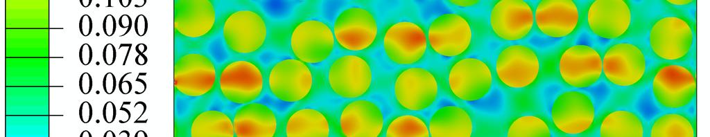
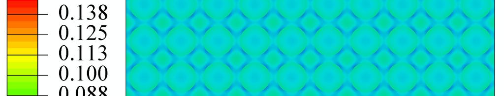
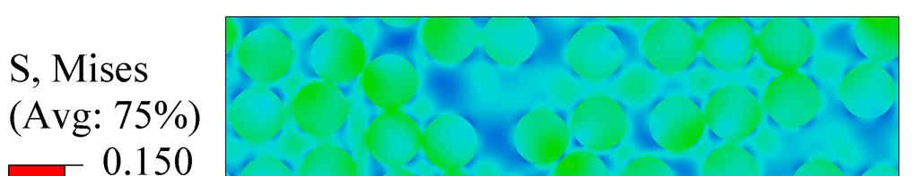
103 (a) Ordered Microstructure (b) Semi-Random Microstructure (c) Hard-Core Microstructure Figure von Mises Stress Contour (GPa) of Unidirectional Composite Loaded in Transverse Tension 83 (a) Ordered Microstructure (b) Semi-Random Microstructure (c) Hard-Core Microstructure Figure von Mises Stress Contour (GPa) of Unidirectional Composite Loaded in Transverse Shear

104 To investigate the effect of fiber geometric variation in comparison to architectural disorder in relation to global composite elastic behaviors, the fiber diameter distribution information obtained in Chapter 3.2.3, was used to create 100 microstructures beginning with an ordered array comprising fibers with a random sampling of fiber diameters and using a Monte Carlo perturbation framework to increase disorder until convergence of the K-function and two-point correlation function was obtained. The microstructures, progressing from ordered to hard-core, were modeled in Abaqus/Standard as triply periodic RUCs and loaded similarly to the microstructures in the previous analysis with constant fiber radii. The predicted global tensile and shear moduli results from these simulations are presented in Figure 3.15, while the von Mises stress contours are shown in Figure 3.16 and Figure 3.17 for tensile and shear loading, respectively. Through the comparison of Figure 3.11 and Figure 3.15 it can observed that the global elastic response of ordered to hard-core microstructures with constant and random fiber diameters demonstrate similar overall trends and final states (i.e., an approximate 5% decrease in tensile modulus and 10% increase in shear modulus). Comparison of the stress contours reveals only subtle differences, including the non-ordered distribution of stress in the ordered fiber array with varying fiber diameters. However, as presented in the previous analysis, the variation in stress concentration has little effect on global properties but may play a larger role when inelastic, local behavior is of interest. From the simulations accounting for fiber position and size variation, it can be concluded that the effect of increasing fiber position randomness has a significantly greater effect on global properties compared to the effect of fiber diameter variation. This conclusion is in agreement with the work presented in Gusev, Hine, and Ward (2000). 84

105 Figure Global Elastic Moduli vs. Microstructural Randomness for Composite RUC Containing Experimentally Determined Distribution of Fiber Radii 85

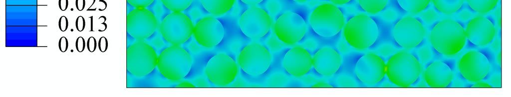
106 (a) Ordered Microstructure (b) Semi-Random Microstructure (c) Hard-Core Microstructure Figure von Mises Stress Contour (GPa) of Unidirectional Composite with Random Distribution of Fiber Radii Loaded in Transverse Tension 86 (a) Ordered Microstructure (b) Semi-Random Microstructure (c) Hard-Core Microstructure Figure von Mises Stress Contour (GPa) of Unidirectional Composite with Random Distribution of Fiber Radii Loaded in Transverse Shear

107 In the previous analyses, the progression of the global tensile modulus was only presented for a single transverse direction (e.g., E11). Given that the perturbation of fiber position will cause deviation from global orthotropic composite response typically assumed for ordered arrangements of fibers, a study was conducted to investigate the degree to which the elastic tensile response differs between the x (i.e., 11) and y (i.e., 22) transverse coordinate directions. The same 100 microstructures were loaded in tension in the 22 direction for the cases of constant and random fiber radii and the results compared to those obtained from loading in the 11 direction, as presented in Figure 3.18 (a) and Figure 3.18 (b), respectively. Observation of the results indicates that there exists little difference in the trend and final state between the elastic properties in the two transverse directions. In fact, the maximum relative difference between the two predicted tensile moduli for the constant and random fiber radii cases are 0.3% and 0.4%, respectively. (a) Composite RUC with Uniform Distribution of Fiber Radii (b) Composite RUC with Random Distribution of Fiber Radii Figure Global Tensile Moduli (E11 and E22) vs. Microstructural Randomness for Composite RUC 87

108 3.3.2 Local Inelastic Composite Behavior Typically, composite elastic properties are governed by the global homogenized stress/strain behavior, while inelastic behavior is governed at a lower local scale where the presence of inclusions promotes diffuse plastic flow. Although the homogenized global fields may be similar between two microstructures, due to the existence of peak stresses and strains in specific regions within the cross section, the inelastic behavior of the microstructures may create drastic differences. Therefore, the effect of decreased spatial order on the local inelastic behavior of the composite was investigated using a similar technique applied in Chapter For this analysis the matrix material was modeled as viscoplastic (as described in formulation presented in Chapter 3.2.2) in order to capture how the local variations in stress and strain fields alter the inelastic behavior of the composite as a function of spatial order. The viscoplastic constitutive relation applied to the matrix material within the FEM framework also allows for the effects of various loading rates to be studied in detail. Four strain rates (1E-3/s, 1E-2/s, 1E-1/s, and 1.00/s) were applied to three simulated microstructures (ordered, semi-random, and hard-core) and loaded in strain control for a total Cauchy strain of 1%. Contours of the effective inelastic strain, computed through the numerical integration of the effective inelastic strain rate in Equation (3.14) over time, are presented for the ordered and hard-core distribution microstructures in Figure 3.19 and Figure 3.20, respectively, for each of the four strain rates. The contours of the effective inelastic strain for the semi-random distribution of fibers are not presented because of their similarities to those for the hard-core distribution. It can be observed that the contour of inelastic strain resembles that of von Mises stress presented in Figure This intuitive 88

109 similarity demonstrates the effect of fiber position variability on the concentration of stresses in regions with fibers aligned favorably with the loading direction and with small interfiber spacing, in addition to the subsequent inelastic behavior initiation and viscoplastic flow. The inelastic behavior of the ordered array (Figure 3.19) retains a regular distribution, while the effective inelastic strain contours for the hard-core microstructure (Figure 3.20) demonstrates regions of significantly higher concentrations. The effect of strain rate can also be observed in the contours presented in Figure 3.19 and Figure As the loading strain rate decreases, the inelastic strains in the matrix increase as a result of the strain rate dependence included in the matrix constitutive relation. These results indicate the importance of accounting for fiber spatial variation when local inelastic behavior is of interest, especially at low strain rates. A qualitative observation of the contours reveals the possibility of under-prediction in the magnitude of inelastic behavior in specific regions if a random microstructure was represented by an ordered array. These results merit additional investigation into the regions of high inelasticity concentrations to better understand the potential shortcomings involved in the simplification of random or experimental microstructures to regular fiber packing arrangements. 89

110 (a) ε&11 = 1E 3 / s (b) ε&11 = 1E 2 / s (c) ε&11 = 1E 1/ s (d) ε&11 = 1.00 / s Figure Effective Inelastic Strain Contour for Ordered RUC 90

111 (a) ε&11 = 1E 3 / s (b) ε&11 = 1E 2 / s (c) ε&11 = 1E 1/ s (d) ε&11 = 1.00 / s Figure Effective Inelastic Strain Contour for Hard-Core RUC Due to the increase in inelastic material behavior concentrations observed for the random microstructures, the regions of maximum effective inelastic strain are investigated in greater detail. This study is expected to further reveal the importance of accounting for architectural variation when accurately capturing the local inelastic behavior is necessary. The maximum effective inelastic (i.e., viscoplastic) logarithmic strain, ε eqvp, is plotted against the applied engineering strain, ε 11, for each of the four strain rates in Figure 3.21, Figure 3.22, and Figure 3.23 for the ordered, semi-random, and hard-core microstructures, respectively. The maximum values of effective inelastic strain, obtained through numerical integration of the effective inelastic strain rate, were 91

112 extracted at each load increment to demonstrate the magnitude of local inelastic behavior as a function of strain rate and microstructural order. As the strain rate decreases for each of the three simulations, it can be observed that the maximum value of effective inelastic strain increases, similar to the qualitative results witnessed in Figure 3.19 and Figure Additionally, as the microstructures progress from ordered to hard-core, the maximum value of effective inelastic strain increases drastically and the variance in the maximum values for the four strain rates also increases. This behavior is a result of the increase in stress concentration surrounding the fibers observed in Figure 3.13 caused by favorable fiber alignment with respect to loading direction and decreased interfiber spacing. The combination of stress concentrations and increased likelihood of resin rich pockets (i.e., particle free regions) promotes the initiation and unimpeded progression of viscoplastic matrix flow because the matrix is allowed to shear freely. Since the progression of inelastic material behavior is significant, investigations that simply quantify the inelastic behavior of ordered verses random microstructures using stress invariants, dilatational energy density, maximum stress and strain, or other elastic field variables to illustrate the increased likelihood of initiation (Wang et al., 2011; Huang, Jin, and Ha, 2008; Trias et al., 2006; Maligno, Warrior, and Long, 2009) do not accurately characterize the more significant and pronounced effect of inelastic behavior progression as a function of increased loading. 92

113 Figure Maximum Effective Inelastic Strain at Four Strain Rates for an Ordered Microstructure Figure Maximum Effective Inelastic Strain at Four Strain Rates for a Semi-Random Microstructure 93

114 Figure Maximum Effective Inelastic Strain at Four Strain Rates for a Hard-Core Microstructure After determining the local effect that fiber position variability plays on the microscale inelastic fields, the focus now lies in how these fields are manifested at the macroscale. The global transverse Cauchy tensile stress versus strain responses of the ordered, semi-random, and hard-core composite microstructures are presented in Figure 3.24 for a strain rate of 1E-3/s. At the global length scale it is observed that local inelastic phenomena have a minimal effect. In fact, at 1% strain, the percent difference in predicted stress for the ordered and hard-core microstructures is only approximately 3.2%. It is evident that as the loading applied to the composite RUCs is increased, the difference in predicted stress responses for the three microstructures also increases. Therefore, if a desired analysis involves large global strains, the effect of local inelastic events will play a more prominent role in the global composite behavior. Similarly, the stress versus strain response for the hard-core microstructure loaded in transverse tension with four strain rates is shown in Figure Comparing the results presented in Figure 3.24 and Figure 3.25, it is evident that strain rate plays a greater role in the global composite behavior than microstructural variability. Given the results for the local 94

115 maximum inelastic strain magnitude and global inelastic stress versus strain behavior, the choice between explicitly analyzing an experimental/random microstructure or assuming order depends on the scale of interest, loading rate, and total applied strain. Figure Cauchy Stress vs. Applied Global Strain from Three Microstructures Loaded at 1E-3/s Strain Rate Figure Cauchy Stress vs. Applied Global Strain for Hard-Core Distribution at Four Strain Rates 95

116 3.3.3 Experimental versus Simulated Microstructures The global and local effects of microstructural (i.e., fiber position) and geometric (i.e., fiber radius) variation have been demonstrated for the cases of elastic and inelastic material behavior and under various loading conditions (i.e., tensile and shear) and strain rates. The next logical step in the analysis involves quantifying the equivalence of the simulated disordered microstructures to those obtained from experimental micrographs. A set of criterion was developed in Liu and Ghoshal (2014a) that provides a systematic approach to determining statistical microstructure equivalence. The first step in the verification process involves simulating a random microstructure with an equivalent fiber volume fraction and fiber radius distribution. Next, it must be verified that the experimental and simulated RVEs are sufficiently large such that the point processes have converged. Lastly, the point processes (e.g., Ripley s K-function) of the experimental and simulated microstructures must be compared for equivalence. If each of the criteria is satisfied within tolerance, the microstructures can be regarded as statistically equivalent. An experimental and a simulated microstructure, both with equivalent fiber volume fraction and radius distribution, are presented in Figure Ripley s K-function was computed for both microstructures and plotted in Figure The apparent similarity between the two K-functions verifies the statistical equivalence of the experimental and simulated microstructures. 96

117 (a) Experimental Microstructure (b) Simulated Microstructure Figure Microstructures for Statistical Equivalence Verification Figure Experimental vs. Simulated Microstructure K- Functions Once the equivalence of experimental and generated microstructures is proven, one question that remains is whether microstructures with identical K-functions have similar elastic behavior. The first step toward addressing this question involves simulating multiple microstructures, each with 324 fibers, and comparing their respective K- functions. It was observed that the K-functions varied by less than 0.1% and had the same volume fractions and distributions for fiber radii; therefore, the microstructures can be considered statistically equivalent. Next, the microstructures were modeled in FEM as 3D triply periodic RUCs and elastic analyses were run for the case of transverse tensile 97

118 loading. The tensile moduli of the generated microstructures were then compared and found to be nearly identical (within 0.5%). This comparison was repeated for 20 microstructures with similar results. These results indicate that the global elastic response of statistically equivalent microstructures, including those obtained from experimental micrographs, will also be equivalent. Since it has been proven that statistical equivalence of microstructures is a good indication of global elastic behavior equivalence, another question that remains is whether the global inelastic behavior is also equivalent for two microstructures with identical K-functions. Two microstructures were simulated and their respective K- functions plotted for comparison, as seen in Figure 3.28 (a). The statistical equivalence of the two microstructures is evident. Using the FEM framework and viscoplastic constitutive model described previously, the two RUCs were simulated in transverse tension up to 1.45% Cauchy strain. The global stress vs. strain behavior of the two microstructures is plotted in Figure 3.28 (b). The mechanical behavior, including inelastic effects, is nearly identical for the two microstructures. These results imply that statistical equivalence of microstructures also can serve as an indication of equivalent mechanical behavior for both elastic and elastic/viscoplastic matrix behavior. 98

119 (a) K-Function (b) Stress vs. Strain Response Figure Statistical and Mechanical Equivalence of Two Simulated Microstructures Finally, an analysis was conducted to investigate whether convergence of the K- function can be correlated to a convergence in global elastic properties. In other words, the goal was to determine whether the elastic behavior of an experimental micrograph with a converged K-function remains stable as further variability is imposed. To provide insight into this question, an experimental microstructure was subjected to the Monte Carlo fiber position perturbation technique (i.e., experimental to hard-core) and simulated with the previously described FEM framework for tensile loading. The tensile modulus was plotted in Figure The relatively small decrease in tensile module (as compared with Figure 3.11) and oscillations witnessed in the plot provide an indication that the elastic properties of the experimental microstructure are nearly stable. Therefore, it can be stated that convergence of the K-function provides a good indication of elastic property convergence. 99

120 Figure Relative Tensile Modulus vs. Microstructural Order (Experimental to Hard-Core) 3.4 Conclusion In this chapter, a comprehensive investigation with the goal of quantifying the local and global effects of microstructural disorder using a 3D micromechanics-based, triply periodic FEM model is presented. Studies were conducted over a variety of fiber arrangements progressing from ordered to hard-core for the purpose of linking the microscale variation and spatial randomness to the macroscale behavior of the composite. Architectural (e.g., fiber position) and geometric (e.g., fiber radius) variations as well as constituent constitutive behavior effects were investigated in detail for transverse loading of the composite microstructures. It was concluded that the importance of considering variations at the microscale depends greatly on the scale and phenomena of interest. For example, for a simple elastic analysis, the effects of microstructural variation are minimal when compared to those from material property or experimental uncertainty. Progressing from ordered to hard-core distributions, the author observed a 5% decrease in the global tensile modulus and a 10% increase in shear modulus. However, if inelastic or small length scale behaviors are of interest, the consideration of microscale variations becomes 100

121 increasingly important for accurately capturing the localized stress concentrations and subsequent initiation and propagation of inelastic behavior. In fact, an 85% error in maximum effective inelastic strain would result from simplification of a hard-core microstructure to one that is ordered. Finally, the results were compared to experimental micrographs and it was concluded that the simulated and experimental microstructures can be considered statistically equivalent and therefore will have similar mechanical behaviors, including inelastic. 101

122 4 FULLY COUPLED ELECTROMECHANICAL ELASTODYNAMIC MODEL FOR GUIDED WAVE PROPAGATION ANALYSIS 4.1 Introduction In order to detect and quantify damage and variability in aerospace metallic and composite structures, there is an urgent need for efficient and accurate monitoring methodologies that can interrogate complex, realistic structures for local damage in realtime without requiring a large number of actuators and sensors. While many NDE approaches have been proven reliable in detecting and quantifying small-scale damage in a variety of materials (Sundararaman, 2007), extension of these techniques to provide feasible and economical in-situ damage monitoring strategies is essential. The real-time monitoring of a structure provides information on the current damage state and can allow maintenance to be performed when needed (i.e., condition-based maintenance (CBM)) rather than when scheduled (i.e., schedule-based maintenance (SBM)). Benefits of transitioning from SBM to CBM include considerable economic savings as well as major improvements to the safety of military and commercial airframes. The current state awareness information can also be used to accurately predict the RUL of the system. Therefore, substantial effort has been dedicated to the development of SHM techniques that can provide the damage detection and quantification features of NDE methods while also offering real-time monitoring capabilities using fewer actuators and sensors (Raghavan and Cesnik, 2007). Among the various techniques used for NDE and SHM of aerospace, civil, and mechanical structures, GW-based techniques have been proven most effective and efficient because of their wide array of applications and sensitivity to multiple types, 102

123 locations, and severities of damage (Raghavan and Cesnik, 2007; Andrews et al., 2008; Giurgiutiu, 2008). One of the most promising GW-based approaches for damage detection in advanced aerospace structures is Lamb wave based techniques (Alleyne and Cawley, 1992; Staszewski et al., 1997; Giurgiutiu, 2008; Jha and Watkins, 2009). Using Lamb wave based approaches for damage detection, localization, and quantification involves exciting the aerospace structure with ultrasonic stress waves using piezoelectric or electromagnetic transducers, collecting the specimen s local vibrational response using sensors, and then processing the received voltage signal for the detection and in-situ characterization of damage. Lamb waves have the ability to travel long distances in platelike structures with minimal attenuation; therefore, SHM techniques utilizing Lamb wave analysis have the potential to monitor large areas with few actuators and sensors (Giurgiutiu, 2008), which minimizes the weight and complexity of the SHM system. The abundance of structures, in particular aerospace structural components, whose profile and mechanical behavior resembles that of thin plates or shells contributes to the vast application of this technique and its feasibility in commercial and military aerospace applications. Piezoelectric transducers are often used to excite and sense Lamb waves in a structure. The direct piezoelectric effect (sensor mode), where the application of strain to the piezoelectric element results in the generation of an electric potential across its poles, and the converse piezoelectric effect (actuator mode), where the application of an electric potential across the poles of the piezoelectric element results in it developing internal strains and therefore stresses, are illustrated in Equations (4.1) and (4.2), respectively, for a linear piezoelectric material (Nayfeh, 1995). When used in the actuator mode, an input 103

124 voltage signal is converted into a strain response that induces an elastic wave in the material while the opposite process is used for sensing the wave. D = e ε + κ σ E, (4.1) i ijk jk ij j and σ = C ε e E, (4.2) E ij ijkl kl kij k where C E is the stiffness tensor measured at zero electric field (i.e., E = 0), κ σ is the dielectric permittivity tensor at zero stress (i.e., σ = 0), e is the piezoelectric tensor, σ is the stress tensor, ε is the strain tensor, D is the electric displacement tensor, and E is the electric field tensor. Therefore, besides their many advantages including light weight, small size, and low cost, another significant benefit of using piezoelectric transducers for Lamb wave structural interrogation is their ability to serve as both an actuator and sensor (Guo and Cawley, 1993; Diaz and Soutis, 2000; Giurgiutiu, 2008). This feature allows a greater number of interrogation scenarios to be investigated, including pulse-echo and pitch-catch methods, with fewer transducers, thereby mitigating weight, cost, and complexity. Lamb wave based techniques have been used by many researchers for damage detection and quantification in both metallic and composite structures; however, most of these methods are experimentally based and data driven (Soni, Das, and Chattopadhyay, 2009; Liu, Mohanty, and Chattopadhyay, 2010; Liu et al., 2011b). Conducting an experiment for every sensor location, wave form type and frequency, and damage type and severity can be prohibitively time-consuming and expensive. The use of hybrid sensing approaches that combine limited experimental data with results from a physics- 104

125 based wave propagation models (referred to as virtual sensing) have been found to be more effective in damage detection of complex aerospace structures (Chattopadhyay et al., 2009). These models provide insight into the damage mechanism, allowing for further optimization of SHM techniques and testing parameters. Additionally, the simulation of 3D Lamb wave propagation through the structure provides high-resolution spatial and temporal information regarding the wave behavior and its interaction with damage, boundaries, and adjacent waves. While similar data can be collected for the surface of the specimen using a laser Doppler vibrometer (LDV), an efficient and accurate simulation approach can provide this information for the interior of the part in addition to the surface. Since damage often initiates within parts and has a 3D morphology (Leckey, Rogge, and Parker, 2014), internal wave propagation information, including reflection and dispersion behavior, is critical in assessing the damage detection and characterization capabilities of various ultrasonic NDE and SHM approaches. The complexity of Lamb waves that are excited and sensed using piezoelectric actuators and sensors for SHM arises from their dispersive nature, existence of at least two GW modes at any excitation frequency, electromechanical coupling due to the piezoelectric phenomenon, interaction with damage and material discontinuities at various length scales, and the 3D nature of the wave propagation problem. It is advantageous, therefore, to have computational models to study the physics of wave propagation, which can aid in the development of accurate damage detection and quantification methodologies. Models for wave propagation also provide a means to interpret the results obtained from experiments in greater detail since the full 105

126 displacement, stress, and strain fields can be studied as opposed to only having access to the sensor signal or surface displacement in the case of experiments. Due to the general limitations associated with analytical wave propagation models for aerospace structures, such as in modeling complex geometries, material architectures, and realistic damage, numerical models are often employed to solve the elastodynamic wave equation for the desired geometry, boundary conditions, actuation signals, and material properties. Numerous numerical techniques exist for modeling elastic wave propagation, such as FEM (Talbot and Przemieniecki, 1975; Zienkiewicz, 1989; Koshiba, Karakida, and Suzuki, 1984), finite strip elements (Cheung, 1976; Liu and Achenbach, 1995; Liu et al., 1999), boundary element method (Yamawaki and Saito, 1992; Cho and Rose, 1996), spectral element methods (Fornberg, 1998; Krawczuk and Ostachowicz, 2001; Hu et al., 2007), and local interaction simulation approach (LISA) / sharp interface model (SIM) (Delsanto et al., 1992; Delsanto et al., 1994; Delsanto, Schechter, and Mignogna, 1997). Although each of these numerical modeling techniques has merit, LISA/SIM is used in this study because of its proven accuracy in simulating ultrasonic elastic wave propagation, including GWs (Delsanto et al., 1992; Delsanto et al., 1994; Delsanto, Schechter, and Mignogna, 1997; Sundararaman, 2007), as well as its computational efficiency (Delsanto, Schechter, and Mignogna, 1997; Borkowski, Liu, and Chattopadhyay, 2013a). In materials with the presence of damage and discontinuities such as cracks, holes, and material interfaces, LISA/SIM has proven to be an effective, accurate, and computationally efficient modeling technique for wave propagation (Agostini et al., 2003; Lee and Staszewski, 2003). One of the main advantages of LISA/SIM is its ability 106

127 to model wave propagation across sharp material property interfaces without incurring significant numerical error caused by the smearing (i.e., averaging) of material properties across interfaces of cells with dissimilar elastic properties (Delsanto et al., 1992; Delsanto et al., 1994; Delsanto, Schechter, and Mignogna, 1997). Lee and Staszewski (2003) modeled Lamb wave based damage detection in metallic specimens using LISA/SIM. Sundararaman (2007) extended the technique to include adaptive grid spacing for higher spatial resolution and flexibility in regions of geometric complexity. Most Lamb wave studies using this technique are carried out on 2D geometries for the reason of computational tractability (Lee and Staszewski, 2003) and limited access to high performance computing resources. Since Lamb waves only exist in 3D bounded media, the 2D models require the Lamb wave group and phase velocities to be provided a priori for the in-plane simulation while the wave propagation in the through-thickness direction is modeled separately. Modeling the inherent 3D problem in this 2D fashion limits the usefulness and accuracy of the model. Therefore in this chapter, a full 3D model is utilized to account for the coupling between the separate Lamb wave modes and to accurately represent the mode conversions and reflections caused by boundaries, damage, or other material discontinuities. While LISA/SIM has been proven to be an effective tool for GW-based SHM, Raghavan and Cesnik (2007) asserted that the application of this technique has been limited due to the lack of a fully coupled electromechanical elastodynamic formulation to account for Lamb wave excitation and sensing using piezoelectric transducers. Accounting for the physics of GW excitation and sensing is crucial to the accurate simulation of wave propagation techniques because of the complex coupling between the 107

128 electrical excitation of the piezoelectric actuator, the subsequent mechanical response of the actuator and structure, and finally the mechanical and electrical response of the sensor. Previous work focused on modeling the excitation of GWs has primarily been based on the theory of elasticity and has utilized the plane strain approximation to simplify the 3D problem to 2D (Viktorov, 1967; Ditri and Rose, 1994). Extensions of the elasticity theory based approaches to 3D have used impulse point body force (Santosa and Pao, 1989) and generic surface point sources (Wilcox, 2004) to model the GW excitation. Relatively little work, however, has been conducted toward the modeling of structurally integrated piezoelectric actuators with finite dimensions. Moulin et al. (2000) modeled a surface-mounted lead zirconate titanate (PZT) transducer using a coupled FEM-normal mode expansion method. Other researchers have also utilized the built-in piezoelectric elements in commercial FEM packages (Soni, Das, and Chattopadhyay, 2009) to model piezoelectric actuators and sensors for SHM applications. Mindlin plate theory incorporating transverse shear and rotary inertia effects was used by other researchers to model the GW excitation as causing bending moments along the actuator edge (Veidt, Liu, and Kitipornchai, 2001; Rose and Wang, 2004). One major disadvantage of using Mindlin plate theory is that it is only capable of approximately modeling the zeroth order antisymmetric Lamb wave mode and therefore is only valid at low frequencies where higher order modes are not present in the plate. Giurgiutiu, Bao, and Zhao (2003) modeled an infinitely wide piezoelectric transducer to study the excitation and propagation of Lamb waves in an isotropic metallic plate. They solved for the displacement and strain fields by first reducing the 3D elasticity problem to 2D using the Fourier integral theorem and then arriving at a solution through 108

129 inversion using residue theory. Raghavan and Cesnik (2005) developed an analytical modeling technique using 3D elasticity theory and the Fourier integral theorem to model actuators and sensors of finite dimensions. This approach was validated experimentally and numerically for the particular cases under investigation. However, the assumption made in the formulation of the analytical approach introduced in Raghavan and Cesnik (2005) limits its application to Lamb wave analysis in infinite plates without considering the effect of the actuator and sensor on structural dynamics and wave behavior since the actuation is modeled as causing an in-plane traction of uniform magnitude only along its perimeter in the direction normal to the free edge of the plate surface. In addition, the plate through-thickness displacement resulting from the Lamb wave propagation is not provided with this approach. In the current chapter, a fully coupled electromechanical elastodynamic model for wave propagation in a heterogeneous, anisotropic material system is developed. To maintain generality, no major assumptions pertaining to geometry, state of stress/strain, material properties, damage, or actuation type were made during model formulation. The objective of developing this novel modeling scheme is to accurately and efficiently study the physics of GW propagation for the purpose of SHM, and in turn, ease the monitoring strategy used for damage detection with GWs. The final set of equations provides the full 3D displacement and electrical potential fields for arbitrary plate and transducer geometries and excitation waveform and frequency. The model framework is based on that developed by Delsanto, Schechter, and Mignogna (1997), but is extended to include piezoelectric coupling and explicit consideration of the piezoelectric actuators and sensors for an anisotropic material system. The model is validated theoretically by 109

130 comparing the simulated Lamb wave group velocity to that predicted by Lamb wave theory (Lamb, 1917) over a wide range of frequency-thickness products. Various studies are conducted to investigate the governing physics of GW analysis for SHM. These studies include investigating the effect of actuation types on sensor signals, relative sensor voltage of Lamb wave modes excited with collocated actuators, and the relationship between the displacement components below the piezoelectric sensor and the sensor voltage. 4.2 Three-Dimensional Electromechanical Coupled Elastodynamic Model Framework This section outlines the derivation of a set of incremental equations for the solution of a fully generalized, fully coupled 3D electromechanical elastodynamic wave propagation model for a heterogeneous, anisotropic material system. The final set of equations will provide the evolution of the time-varying displacement and electric potential fields for an arbitrary geometry and actuation waveform. This formulation solves the elastodynamic wave equations (classified as hyperbolic partial differential equations (PDEs)) as an initial value problem and the electrostatic Maxwell s equations (classified as elliptic PDEs) as a boundary value problem at each time step and for each grid point. Through the simultaneous solution of Equations (4.1) and (4.2) representing the direct and converse piezoelectric effects, respectively, the two-way coupling present in piezoelectric actuation and sensing of Lamb waves are accounted for accurately Governing Equations and Discretization In this approach, the spatial domain is discretized in the x, y, z Cartesian directions into a cuboidal grid with dimensions x, y, and z, respectively, as shown in Figure

131 The material properties of each cell are defined at the node with the lowest coordinate value within each cell (i.e., the node closest to the origin), meaning an element with its center at location ( α x/2, β y/2, z/2) will have its mechanical and physical properties defined at ( α, β, ). While the material properties are constant within each cell, they are allowed to vary across cells. The incorporation of SIM into the LISA framework allows for the accurate simulation of wave propagation across sharp material boundaries since the material properties are not required to be smeared across cell interfaces to ensure stability of the solution. In order to enforce continuity of displacement at the nodes and traction across the interfaces, points are defined in the grid at infinitesimal distances δ and ι from the nodal points and the interface, denoted by a cross and a star in Figure 4.1, respectively. The distances δ and ι are exaggerated in Figure 4.1 for clarity. Figure 4.1. Definition of Nodal Points and Supplemental LISA/SIM Grid Points 111

132 The constitutive relations and electromagnetic governing equations for a linear piezoelectric continuum material can be found in ANSI/IEEE (1987). For a linear elastic piezoelectric material, the constitutive equation that governs the interaction of the elastic and electric fields can be written as σ = C ε e E, (4.3) ij ijkl kl kij k where σij, Cijkl, εkl, ekij, and Ek are components of the second order stress tensor, fourth order stiffness tensor, second order strain tensor, third order piezoelectric tensor, and first order electric field tensor, respectively. The components of the electric displacement vector can be expressed in terms of the strain and electric field in the form D = e ε + κ E, (4.4) i ijk jk ij j where Di is a component of the first order electric displacement tensor and κij is a component of the second order dielectric tensor. The components of the small strain tensor εkl are expressed in terms of the displacement components uk using the strain-displacement relation, 1 ε kl = ( uk, l + ul, k ), (4.5) 2 and the components of the electric field Ei can be obtained from the electric potential φi via E i = φ. (4.6), i Using the strain-displacement relation (Equation (4.5)), definition of electric field (Equation (4.6)), and the symmetry of the stiffness tensor, Equations (4.3) and (4.4) can be expressed in terms of displacement and electric potential as 112

133 σ ij = Cijkluk, l + ekijφ, k (4.7) and D = e u κ φ. (4.8) i ijk j, k ij, j In a piezoelectric elastic medium, the relationship between and evolution of nodal displacement and electric potential are governed by the elastodynamic wave equation in the form C u + e φ = ρu&&. (4.9) ijkl k, jl kij, kj i It should be noted that viscoelasticity was not included in the current work since it has been investigated by previous researchers, such as Sundararaman (2007). In the absence of volume charges, Maxwell s equation, D = 0, (4.10) must be satisfied, which for a piezoelectric linear elastic material requires e u =. (4.11) ijk j, ki κijφ, ji 0 A central difference scheme is used to approximate the second order derivatives of the displacement and electrical potential at points defined at small distances from the node (i.e., ( α aδ, β bδ, cδ ) ) in the cuboidal grid in terms of their first order derivatives. Here, a, b, c represent neighboring nodes and have the value of ±1, ±1, ±1, respectively, while δ represents a small distance away from the node. The finite difference expressions for the second order differential equations are supplied here for clarity. 113

134 u u α + a/2, β, α + aδ, β + bδ, + cδ α + aδ, β + bδ, + cδ uk,1 uk,1 k,11 = a x/2 α + a, β + b/2, α, β + b/2, α + aδ, β + bδ, + cδ α + aδ, β + bδ, + cδ uk,2 uk,2 k,12 = uk,21 = u a x α, β + b/2, α + aδ, β + bδ, + cδ α + aδ, β + bδ, + cδ uk,2 uk,2 k,22 = b y/2 (4.12) (4.13) (4.14) u α, β + b, + c/2 α, β, + c/2 α + aδ, β + bδ, + cδ α + aδ, β + bδ, + cδ uk,3 uk,3 k,23 = uk,32 = b y (4.15) u φ u α, β, + c/2 α + aδ, β + bδ, + cδ α + aδ, β + bδ, + cδ uk,3 uk,3 k,33 = c z/2 α + a/2, β, + c α + a/2, β, α + aδ, β + bδ, + cδ α + aδβ + bδ, + cδ uk,1 uk,1 k,13 = uk,31 = φ c z α + a/2, β, α + aδ, β + bδ, + cδ α + aδ, β + bδ, + cδ φ,1 φ,1,11 = a x/2 α + a, β + b/2, α, β + b/2, α + aδ, β + bδ, + cδ α + aδ, β + bδ, + cδ φ,2 φ,2,12 = φ,21 = φ a x α, β + b/2, α + aδ, β + bδ, + cδ α + aδ, β + bδ, + cδ φ,2 φ,2,22 = b y/2 (4.16) (4.17) (4.18) (4.19) (4.20) φ α, β + b, + c/2 α, β, + c/2 α + aδ, β + bδ, + cδ α + aδ, β + bδ, + cδ φ,3 φ,3,23 = φ,32 = b y (4.21) φ φ α, β, + c/2 α + aδ, β + bδ, + cδ α + aδ, β + bδ, + cδ φ,3 φ,3,33 = c z/2 α + a/2, β, + c α + a/2, β, α + aδ, β + bδ, + cδ α + aδ, β + bδ, + cδ φ,1 φ,1,13 = φ,31 = c z (4.22) (4.23) 114

135 Similarly, the first order derivatives of displacement and electric potential at points ( α + a/2, β, ), ( α, β + b/2, ), and ( α, β, + c/2) difference. are also expressed using finite u α + a, β, α, β, α + a/2, β, uk uk k,1 = a x (4.24) u α, β + b, α, β, α, β + b/2, uk uk k,2 = b y (4.25) u φ α, β, + c α, β, α, β, + c/2 uk uk k,3 = c z α + a, β, α, β, α + a/2, β, φ φ,1 = a x α, β + b, α, β,, + b/2,,2 = α β φ φ φ b y (4.26) (4.27) (4.28) φ α, β, + c α, β, α, β, + c/2 φ φ,3 = c z (4.29) Next, continuity of displacement and electric potential will be enforced at additional points defined at a small distance from the grid points. A very small distance, denoted by ι, will be defined as ι = δ x, x >> 1. (4.30) The first order spatial derivatives of displacement (Delsanto, Schechter, and Mignogna, 1997) used for enforcing continuity of displacement are presented in Equations (4.31) through (4.39) for clarity. Similarly, the first order spatial derivatives of electric potential utilized for the enforcement of the continuity of electric potential are shown in Equations (4.40) through (4.48). 115

136 u α + aι, β + bδ, + cδ k,1 = u α + aδ, β + bδ, + cδ k,1 (4.31) u α + aδ, β + bι, + cδ k,1 u = u a x α + a, β, α, β, k k (4.32) u α + aδ, β + bδ, + cι k,1 u = u a x α + a, β, α, β, k k (4.33) u α + aι, β + bδ, + cδ k,2 u = u b y α, β + b, α, β, k k u α + aδ, β + bι, + cδ k,2 = u α + aδ, β + bδ, + cδ k,2 u α + aδ, β + bδ, + cι k,2 u = u b y α, β + b, α, β, k k (4.34) (4.35) (4.36) u α + aι, β + bδ, + cδ k,3 u = α, β, + c α, β, k uk (4.37) c z u α + aδ, β + bι, + cδ k,3 u = α, β, + c α, β, k uk (4.38) c z u α + aδ, β + bδ, + cι k,3 = u α + aδ, β + bδ, + cδ k,3 (4.39) φ α + aι, β + bδ, + cδ,1 = φ α + aδ, β + bδ, + cδ,1 (4.40) φ α + aδ, β + bι, + cδ,1 φ = φ a x α + a, β, α, β, (4.41) φ α + aδ, β + bδ, + cι,1 φ = φ a x α + a, β, α, β, (4.42) φ α + aι, β + bδ, + cδ,2 φ = φ b y α, β + b, α, β, φ α + aδ, β + bι, + cδ,2 = φ α + aδ, β + bδ, + cδ,2 φ α + aδ, β + bδ, + cι,2 φ = φ b y α, β + b, α, β, (4.43) (4.44) (4.45) φ α + aι, β + bδ, + cδ,3 φ = φ c z α, β, + c α, β, (4.46) φ α + aδ, β + bι, + cδ,3 φ = φ c z α, β, + c α, β, (4.47) φ α + aδ, β + bδ, + cι,3 = φ α + aδ, β + bδ, + cδ,3 (4.48). The expressions for the first order derivatives of displacement in Equations (4.31), (4.35), and (4.39) and for electric potential in Equations (4.40), (4.44), and (4.48) remain 116

137 unknown. To solve for equilibrium and Maxwell s equation, continuity of tractions and electric displacement across the element interfaces are enforced. This will allow for the unknown first order derivatives to be eliminated Enforcement of Elastodynamic Equilibrium and Continuity of Traction The elastodynamic equilibrium equations at the points ( α aδ, β bδ, cδ ) expressed as can be C u + e α + aδ, β + bδ, + cδ α + aδ, β + bδ, + cδ α + aδ, β + bδ, + cδ α + aδ, β + bδ, + cδ ijkl k, lj lij, lj = ρ u&& α + aδ, β + bδ, + cδ α + aδ, β + bδ, + cδ i φ (4.49) for a, b, c = ±1. The stress tensor at points near the nodes can be expressed as σ = C u + e φ (4.50) α + aδ, β + bδ, + cδ α + aδ, β + bδ, + cδ α + aδ, β + bδ, + cδ α + aδ, β + bδ, + cδ α + aδ, β + bδ, + cδ ij ijkl k, l lij, l for a, b, c = ±1. Next, traction continuity is imposed across the cell interfaces at points near the nodes while recalling that the material properties (e.g., stiffness tensor, density, piezoelectric tensor, and dielectric tensor) are constant in each cell, for example, C = C = C = C = C. (4.51) α + ι, β + δ, + δ α + δ, β + ι, + δ α + δ, β + δ, + ι α + δ, β + δ, + δ α, β, ijkl ijkl ijkl ijkl ijkl Since the cell faces are orthogonal and aligned, the tractions can be expressed directly as the stress tensor. The vector equations can be expressed in compact form as σ = σ (4.52) α ι, β + bδ, + cδ α + ι, β + bδ, + cδ i1 i1 σ = σ (4.53) α + aδ, β ι, + cδ α + aδ, β + ι, + cδ i2 i2 σ = σ (4.54) α + aδ, β + bδ, ι α + δ, β + bδ, + ι i3 i3 for a, b, c = ±1. 117

138 4.2.3 Final Expressions for Nodal Mechanical Displacement After substituting the expressions for stress into Equations (4.52),(4.53), and (4.54), replacing the first and second order spatial derivatives with their respective finite difference expressions in Equations (4.49) and (4.50), and summing over a, b, and c, the unknown first order derivatives can be eliminated through a linear combination of the traction continuity and equilibrium equations. The time derivatives of the displacement are then expanded using finite difference and the final expression for the nodal displacement at time t+ t is achieved, as presented in Equations (4.55) through (4.59). The solution of displacement at any point at time t+ t, solved using forward integration, is a function of the material properties of the surrounding elements and the displacement and electric potential of the surrounding nodes at time t and t- t. where 2 α, β,, t + 1 α, β,, t α, β,, t 1 δt u = 2u u + f + g + h i i i a, b, c=± 1 8ρ a, b, c =± 1 ( ) (4.55) 1 s ρ = ρ, (4.56) 8 and f and f f f = x y z x y z ( α +, β, α, β, ) α + ( φ, β, α, β, φ ) ( α, β +, α, β, ) α, β +, ( φ α, β, φ ) ( α, β, + α, β, ) α, β, + ( φ α, β, φ ) f = C u u + e s a s a x i1k1 k k 11 i f = C u u + e s b s b y i2k2 k k 2i2 f = C u u + e s c s c z i3k3 k k 3i3, (4.57) 118

139 gxy g g xz yx gyz g g zx zy g = ab x y ac x z ab x y bc y z ac x z bc y z s α, β + b, α, β, s α, β + b, α, β, = 1 2 ( ) + 21 ( φ φ ) s α, β, + c α, β, s α, β, + c α, β, = 1 3 ( ) + 31 ( φ φ ) s α + a, β, α, β, s α + a, β, α, β, = 2 1 ( ) + 12 ( φ φ ) s α, β, + c α, β, s α, β, + c α, β, = 2 3 ( ) ( φ φ ) s α + a, β, α, β, s α + a, β, α, β, = 3 1 ( ) + 13 ( φ φ ) s α, β + b, α, β, s α, β + b, α, β, = 3 2 ( ) ( φ φ ) g C u u e xy i k k k i g C u u e xz i k k k i g C u u e yx i k k k i g C u u e yz i k k k i g C u u e zx i k k k i g C u u e zy i k k k i, (4.58) and h h h hyz ab x y ac x z bc y z xy xz = + + s s α + a, β + b, α + a, β, α, β + b, α, β, ( )( ) s s α + a, β + b, α + a, β, α, β + b, α, β, ( e1 i2 + e21 i )( φ φ φ + φ ) s s α + a, β, + c α + a, β, α, β, + c α, β, ( )( ) s s α + a, β, + c α + a, β, α, β, + c α, β, ( e13 i + e3i 1)( φ φ φ + φ ) s s α, β + b, + c α, β + b, α, β, + c α, β, ( )( ) s s α, β + b, + c α, β + b, α, β, + c α, β, ( e2i3 + e3i2 )( φ φ φ + φ ) h = C + C u u u + u + xy i k i k k k k k h = C + C u u u + u +, xz i k i k k k k k h = C + C u u u + u + yz i k i k k k k k (4.59) where superscript s denotes the point ( α aδ, β bδ, cδ ) Enforcement of Maxwell s Equation and Continuity of Electric Displacement A similar approach is applied to derive an expression for the electric potential at time t. First, Maxwell s equation (Equation (4.10)) is enforced at every point ( α aδ, β bδ, cδ ) as e κ φ = (4.60) α + a δ, β + b δ, + c δ α a, b, c a, b, c a, b, c ijk u + δ β + δ + δ α + δ β + δ + δ α + δ β + δ + δ j, ki ij, ji 0 for a, b, c = ±1. The electric displacement tensor at points near the nodes can be expressed as 119

140 D = e u κ φ (4.61) α aδ, β bδ, cδ α aδ, β bδ, cδ α aδ, β bδ, cδ α aδ, β bδ, cδ α aδ, β bδ, cδ i ijk j, k ij, j for a, b, c = ±1. Next, the continuity of the normal electric displacements are enforced at infinitesimal distances from the interface, resulting in the following vector equations, D = D (4.62) α + ι, β + bδ, + cδ α ι, β + bδ, + cδ 1 1 D = D (4.63) α + aδ, β + ι, + cδ α + aδ, β ι, + cδ 2 2 D = D (4.64) α + aδ, β + bδ, + ι α + aδ, β + bδ, ι 3 3 for a, b, c = ± Final Expressions for Nodal Electrical Potential After substituting the expressions for electric displacement into Equations (4.62), (4.63), and (4.64), replacing the first and second order spatial derivatives with their respective finite difference expressions in Equations (4.60) and (4.61), and summing over a, b, and c, the unknown first order derivatives can be eliminated through a linear combination of the electric displacement continuity and Maxwell s equation. After simplification, the final expression for the electric potential at time t is achieved, as seen in Equations (4.65) through (4.68). The solution of electric potential at any point at time t is a function of the material properties of the surrounding elements and the displacement and electric potential of the surrounding nodes at time t. Since the coupled equation for electric potential at the point ( α, β, ) at the current time step is dependent on the electric potential of the nodes surrounding the point ( α, β, ) at the current time step, the solution of the boundary value problem requires the simultaneous solution of a set of 120

141 dependent equations. In this work, LU decomposition was utilized to solve for the electric potential to ensure numerical accuracy, convergence, and efficiency. ( q + r + s) = 0 (4.65) a, b, c=± 1 where q q x y qz q = x y z and α +, β, α, β, α +, β, α, β, ( u ) κ ( φ φ ) α, β +, α, β, α, β +, α, β, ( ) κ ( φ φ ) α, β, + α, β, α, β, + α, β, ( u ) κ ( φ φ ) q = e u s a s a x 1j1 j j 11 q = e u u s b s b y 2 j2 j j 22 q = e u s c s c z 3j3 j j 33, (4.66) rxy r r xz yx ryz r r zx zy r = ab x y ac x z ab x y bc y z ac x z bc y z ( α, β +, α, β, ) α, β +, κ ( φ α, β, φ ) ( α, β, + α, β, ) α, β, + κ ( φ α, β, φ ) ( α +, β, α, β, ) α + κ ( φ, β, α, β, φ ) ( α, β, + α, β, ) α, β, + κ ( φ α, β, φ ) ( α +, β, α, β, ) α + κ ( φ, β, α, β, φ ) ( α, β +, α, β, ) α, β +, κ ( φ α, β, φ ) r = e u u s b s b xy 1j2 j j 12 r = e u u s c s c xz 1j3 j j 13 r = e u u s a s a yx 2 j1 j j 21 r = e u u s c s c yz 2j3 j j 23 r = e u u s a s a zx 3j1 j j 31 r = e u u s b s b zy 3j2 j j 32, (4.67) and 121

142 s s s syz ab x y ac x z bc y z xy xz = + + s s α + a, β + b, α + a, β, α, β + b, α, β, ( )( ) s s α + a, β + b, α + a, β, α, β + b, α, β, ( κ12 + κ21)( φ φ φ + φ ) s s α + a, β, + c α + a, β, α, β, + c α, β, ( )( ) s s α + a, β, + c α + a, β, α, β, + c α, β, ( κ13 + κ31 )( φ φ φ + φ ) s s α, β + b, + c α, β + b, α, β, + c α, β, ( )( ) s s α, β + b, + c α, β + b, α, β, + c α, β, ( κ23 + κ32 )( φ φ φ + φ ) s = e + e u u u + u xy j j j j j j s = e + e u u u + u, xz j j j j j j s = e + e u u u + u yz j j j j j j (4.68) where superscript s denotes the point ( α aδ, β bδ, cδ ) Simulation Results and Discussion Physical Model Development A 247 mm x 247 mm x 4 mm aluminum plate with collocated actuators and a single sensor, as seen in Figure 4.2, was modeled for the various studies presented in this work. The actuators and sensors were centered on the plate and separated by a distance of 22 mm. The aluminum plate was modeled as a homogeneous, isotropic material with a density of 2780 kg/m 3, Young s modulus of 70 GPa, and Poisson s ratio of 0.3. The orthotropic material properties of the PZT piezoelectric actuators and sensors are presented in Table 4.1. A 5 cycle cosine tone burst signal, seen in Figure 4.3, was used to excite the PZT actuators with a maximum electric potential of 10 V. A tone burst signal is utilized to minimize the spectral bandwidth of the signal while maintaining ease of time-of-flight (ToF) determination in Lamb wave based SHM (Kessler, 2002; Raghavan and Cesnik, 2007). 122

143 Figure 4.2. Simulated Plate Geometry (Not to Scale) Table 4.1. PZT (APC 850) Orthotropic Properties Elastic Properties Elastic Moduli Shear Moduli Poisson s Ratio (GPa) (GPa) E n G E n G E n G Density (kg m -3 ) 7500 Piezoelectric Properties (C m -2 ) e e e e e e e e e e e e e e e e e e Dielectric Properties (C V -1 m -1 ) κ e-8 κ e-8 κ e-8 123

144 Figure Cycle Cosine Tone Burst Excitation Computation issues that must be considered when implementing the current numerical framework for wave propagation modeling are convergence, numerical dispersion, and pulse and amplitude distortions. Several factors contribute to these issues. Pulse distortion, for example, can be mitigated through the use of a stable time step that satisfies the Courant Friedrich Lewy (CFL) condition, Equation (4.69) CFL = cmax t + + 1, (4.69) x y z where cmax is the maximum wave speed (i.e., longitudinal wave speed), t is the time step (i.e., sampling period), and x, y, z are the grid spacings for the cuboid elements (Virieux, 1986). To prevent amplitude distortion, the general criterion is to have at least eight elements per minimum wavelength (Balasubramanyam et al., 1996) as seen in Equation (4.70). It is also commonly advised to avoid having more than twenty elements per minimum wavelength to avoid computational issues such as long run times and numerical error associated with the propagation of round-off error (Alleyne and Cawley, 1991). The grid spacings (i.e., x, y, and z) and time step (i.e., t) for the studies 124

145 presented in this chapter were chosen to ensure convergence while minimizing numerical error and computational burden. The grid spacings in the x, y, and z directions were held at 1 mm while the time step was adjusted to satisfy the CFL criterion. c 8f min x, y, z, (4.70) max where cmin is the minimum wave speed and fmax is the maximum frequency Theoretical Validation The fully coupled electromechanical model was validated theoretically by simulating a 4 mm thick aluminum plate with collocated PZT actuators and a single PZT sensor. The Lamb wave governing equations (Lamb, 1917) are presented in Equation (4.71) where the ±1 exponent indicates the symmetric and antisymmetric Lamb wave modes, respectively. The governing equations were solved numerically using the technique outlined in Rose (2004). The phase and group velocities can be then solved using Equations (4.74) and (4.75). 2 tan( βb/2) 4αβk = tan( αb/2) ( k β ) ± 1 (4.71) where ω α =, (4.72) k 2 cl ω β =, (4.73) k 2 ct 125

146 and ω is the angular frequency, k is the wave number, cl is the longitudinal wave speed, ct is the transverse wave speed, and b is the plate thickness. The equations for the Lamb wave group and phase velocities are c p ω = and (4.74) k c g dω =. (4.75) dk By utilizing collocated actuators, Lamb wave mode suppression can be controlled which allows certain modes to be excited selectively. This technique therefore permits direct comparison between the simulated results and the theoretical dispersion curve for an aluminum plate over a range of frequencies commonly utilized for SHM. In addition to the commonly used frequency-thickness products, simulations at additional frequencies were carried out to prove that the model can accurately predict the Lamb wave group velocity at higher frequency-thickness products as well. Giurgiutiu (2005) analytically determined that there is a limited frequency range in which the energy of the S0 mode is greater than that of the A0 mode. Because of this, collocated actuators are necessary for comparing the simulated S0 group velocity to that predicted with Lamb wave theory without the need for complex signal processing. Since the time-of-arrival of the A0 and S0 Lamb wave modes is a common feature used in SHM damage detection methodologies, wave propagation models for this purpose must be able to accurately predict the wave speed of these zeroth order modes. Figure 4.4 presents a comparison between the simulated group velocities (cg) vs. the frequency-half thickness product (fb/2) with the theoretical A0 and S0 group velocities. From this figure, it is evident that the developed model is able to accurately predict the group velocity dispersive trend of 126

147 the two zeroth order Lamb wave modes. The discrepancies between the simulated and theoretical wave speed for some of the frequency-half thickness products investigated may be attributed to grid dispersion caused by insufficient spatial samples per wavelength. Additionally, because of the finite bandwidth of the simulated wave and the dispersive nature of Lamb waves, the energy packet will spread as time progresses in the simulation, leading to errors in the predicted wave speed. While the physical dispersion of the wave packet is unavoidable, the numerical dispersion can be mitigated by decreasing the spatial discretization size. Figure 4.4. Theoretical Validation of A0 and S0 Lamb Wave Mode Group Velocities The two fundamental Lamb wave modes have distinct displacement signatures in the through-thickness plane of the plate. Lamb waves have the unique characteristic of resembling a standing wave through the thickness and a traveling wave in-plane. Figure 4.5 demonstrates this phenomenon as well as illustrating the concept of collocated PZT actuation for mode suppression. For symmetric Lamb wave modes, the out-of-plane displacement profile is symmetric while the in-plane displacement is antisymmetric with respect to the mid-plane of the plate. For antisymmetric Lamb wave modes, the opposite is true. By plotting the out-of-plane and in-plane displacement contours and displacement 127

148 vectors at each node for the A0 and S0 modes, the characteristic displacement profiles of each mode can be visualized and compared as seen in Figure 4.6 through Figure 4.9 for two simulation times ( µs and µs). These two simulation times were chosen because the displacement profile at these times best illustrates the unique propagation characteristics of Lamb waves. In these figures, the Lamb waves were excited from the center of the plate using collocated PZT actuators and propagated outward as illustrated by the arrows. It should be noted that the contours are not to scale as they have been rescaled to clearly demonstrate the through-thickness displacement profile of Lamb waves. The contours of out-of-plane and in-plane displacement and the vector plot of each fundamental Lamb wave mode at the two simulation times demonstrate the unique displacement profile of Lamb wave modes and highlight the ability of the developed wave propagation methodology to provide valuable high resolution spatial and temporal physical information not accessible via SHM experiments, even with advanced hardware such as LDV. 128

149 Figure 4.5. Relative Actuator Voltage Poling Directions and Resultant Through- Thickness Displacement Profile (Out-of-Plane) for Collocated Piezoelectric Actuation for Selective Lamb Wave Mode Suppression 129

150 Propagation (a) Through-Thickness Out-of-Plane Displacement (u3) Contour of A0 Lamb Wave Mode Propagation 130 (b) Through-Thickness In-Plane Displacement (u2) Contour of A0 Lamb Wave Mode Propagation (c) Through-Thickness Vector Plot (u2, u3) of A0 Lamb Wave Mode Figure 4.6. Through-Thickness Plots of (a) Out-of-Plane Displacement, (b) In-Plane Displacement, and (c) Vector Field for A0 Lamb Wave Mode at t= µs for fb/2=300 khz-mm

151 Propagation (a) Through-Thickness Out-of-Plane Displacement (u3) Contour of S0 Lamb Wave Mode Propagation 131 (b) Through-Thickness In-Plane Displacement (u2) Contour of S0 Lamb Wave Mode Propagation (c) Through-Thickness Vector Plot (u2, u3) of S0 Lamb Wave Mode Figure 4.7. Through-Thickness Plots of (a) Out-of-Plane Displacement, (b) In-Plane Displacement, and (c) Vector Field for S0 Lamb Wave Mode at t= µs for fb/2=300 khz-mm

152 Propagation (a) Through-Thickness Out-of-Plane Displacement (u3) Contour of A0 Lamb Wave Mode Propagation 132 (b) Through-Thickness In-Plane Displacement (u2) Contour of A0 Lamb Wave Mode Propagation (c) Through-Thickness Vector Plot (u2, u3) of A0 Lamb Wave Mode Figure 4.8. Through-Thickness Plots of (a) Out-of-Plane Displacement, (b) In-Plane Displacement, and (c) Vector Field for A0 Lamb Wave Mode at t=33.25 µs for fb/2=300 khz-mm

153 Propagation (a) Through-Thickness Out-of-Plane Displacement (u3) Contour of S0 Lamb Wave Mode Propagation 133 (b) Through-Thickness In-Plane Displacement (u2) Contour of S0 Lamb Wave Mode Propagation (c) Through Thickness Vector Plot (u2, u3) of S0 Lamb Wave Mode Figure 4.9. Through-Thickness Plots of (a) Out-of-Plane Displacement, (b) In-Plane Displacement, and (c) Vector Field for S0 Lamb Wave Mode at t=33.25 µs for fb/2=300 khz-mm

154 4.3.3 Computational Efficiency The LISA/SIM solution methodology was initially formulated to run in a highly parallel processing environment on connection machines where each material cell and corresponding grid points would be in a one-to-one correspondence with the processors executed using a single instruction, multiple data (SIMD) approach (Delsanto et al., 1992). Hence, the computational efficiency of the current model offers key advantages over other wave propagation models that must either operate on serial computational architectures or cannot be parallelized to the same degree. A 247 x 247 x 4 mm aluminum plate with one actuator and one sensor was modeled using both the developed model and the commercial FEM software Abaqus (2009). Both models were run in a parallel computing environment on eight Harpertown 2.66 GHz, 8 MB/Cache, 16 GB memory processors. Each model was run in double precision for 1000 time increments with a time step of 9.5e-8 s. The computation results, including wallclock time, are shown in Table 4.2. Although the number of elements required for the current model was more than twice that required for the FEM model due to the way in which boundary conditions are applied in LISA/SIM, the current model was significantly faster (>170 times) than the comparable FEM model. Using a time step of 9.5e-8 s, numerical instability occurred in the FEM model of the plate and a time step of 3e-8 s was required to resolve the issue of numerical instability. In addition, the FEM model underpredicted the theoretical wave speed by 13.3% for a time step of 3e-8 s while the result using the current model was within 4.1% for a time step of 9.5e-8 s. 134

155 Table 4.2. Computational Efficiency Comparison between FEM and Current Model Solver Method # of elements Wallclock time (s) FEM 244,038 40,855 Current Model 567, Collocated Actuators for Selective Lamb Wave Mode Suppression Collocated piezoelectric actuators have been utilized experimentally to selectively suppress Lamb wave modes for the purpose of SHM (Kim and Sohn, 2007). The suppression of one of the two fundamental Lamb wave modes is achieved by selectively poling the collocated piezoelectric actuators, indicated with the black arrows in Figure 4.5. In SHM, it is often desired to excite a wave with predominately symmetric or antisymmetric behavior to facilitate time-of-arrival calculation or to tailor the Lamb wave excitation to a specific type and location of damage in the structure. Although this phenomenon has been proven theoretically and successfully implemented experimentally (Kim and Sohn, 2007), it is often difficult to replicate experimentally. Slight variance in the relative actuator placement or in the piezoelectric actuator properties can have a significant impact on the degree of mode suppression. Therefore, numerical wave propagation models offer a valuable tool in investigating the physics of this experimental technique. The ability to separately model the fundamental Lamb wave modes is necessary for understanding the role each mode plays in the overall propagation of the Lamb wave and its interaction with damage and other features. Simulation results may 135

156 also provide insight into methods to improve the feasibility of collocated PZT actuation for experimental damage detection and characterization. Giurgiutiu (2005) demonstrated the concept of Lamb wave mode tuning using a single actuator, which involves exciting the structure with a frequency at which the A0 or S0 mode is most prevalent (i.e., largest relative energy). This type of selective tuning is possible because the relative energy of the fundamental Lamb wave modes vary with frequency. Although mode tuning using a single piezoelectric actuator has been proven feasible, larger suppression of the undesired mode can be achieved with collocated actuators. Numerical models can be called to investigate the physics and provide insight into the problem before experimental implementation occurs. For damage detection using Lamb waves, it is desirable to excite a mode with the largest possible energy. Since the use of collocated actuators cannot completely eliminate the undesired mode, it is beneficial to know the frequency at which the maximum difference between the mode energies occurs. For homogeneous, isotropic specimens, an analytical technique such as the one utilized by Kim and Sohn (2007) and Giurgiutiu (2005) can predict the relative mode energies; however, for specimens with complex heterogeneous architectures and anisotropy, numerical models such as the one presented in the current work are required. To demonstrate the concept, a 4 mm thick aluminum plate was modeled with collocated actuators and a single sensor. Through modeling collocated actuators to selectively excite a single mode at various frequencies and overlaying the sensor voltage results, the relative sensor energies can be compared, as seen in Figure 4.10 (a), Figure 4.10 (b), Figure 4.10 (c), and Figure 4.10 (d) for the frequency-half thickness products (fb/2) of 200 khz-mm, 300 khz-mm, 400 khz-mm, and 500 khz-mm, respectively. 136

157 (a) Sensor Voltage vs. Time for fb/2 = 200 khz-mm (b) Sensor Voltage vs. Time for fb/2 = 300 khz-mm (c) Sensor Voltage vs. Time for fb/2 = 400 khz-mm (d) Sensor Voltage vs. Time for fb/2 = 500 khz-mm Figure Comparison of Sensor Voltage between Symmetric and Antisymmetric Zeroth Order Lamb Wave Modes for fb/2 Equal to (a) 200 khz-mm, (b) 300 khz-mm, (c) 400 khz-mm, and (d) 500 khz-mm Figure 4.10 demonstrates the dependence of Lamb wave displacement amplitudes on excitation frequency and the change in the relative amplitudes of the zeroth order modes as a function of frequency-thickness product. At the frequency-half thickness product of 200 khz-mm, the A0 mode is more prevalent (i.e., has a higher relative energy) than the S0 mode. As the frequency-thickness product increases, the relative energy of the S0 mode increases until it is the dominant mode as seen in Figure 4.10 (d) for a frequency- 137

158 thickness product of 500 khz-mm. A systematic study such as the one presented in Figure 4.10 can be used to improve experimental damage detection techniques and tailor excitation frequencies to best suit the type and location of damage in a specific part or structure based on material system, geometry, and damage type and location Effect of Actuation Type Prior to the development of the fully coupled electromechanical theory for LISA/SIM, researchers modeling piezoelectric actuation (Lee and Staszewski, 2003; Sundararaman, 2007) were forced to apply displacements to the piezoelectric nodes or the cells beneath the actuator. In a study on the excitation of surface-bonded piezoelectric transducers, Giurgiutiu, Bao, and Zhao (2003) noted that the actuators typically used for SHM operated in a pinching fashion or by causing a traction tangent to the plate surface. Most researchers found that application of an actuation in the form of a displacement in the in-plane direction gave more accurate prediction of wave speeds. However, this type of actuation does not take into consideration the complex piezoelectric coupling occurring within the actuator that causes the application of traction to the plate surface as a result of the externally supplied voltage across the actuator surfaces. To investigate the effects of representing the piezoelectric actuation with applied displacement on the subsequent wave signature, a detailed numerical investigation is necessary. A study was conducted to investigate the effect of and error incurred due to displacement actuation compared to explicitly modeling the piezoelectric device. Three commonly used actuation types were investigated: displacement in the y-direction (inplane) actuation, displacement in the z-direction (out-of-plane) actuation, and electrical 138

159 actuation, as shown in Figure The sensor signals for the A0 and S0 Lamb wave modes actuated using three different actuations are shown in Figure 4.12 (a) and Figure 4.12 (b), respectively, for fb/2 equal to 300 khz-mm. It is evident from the plots that the time-of-arrival and wave speed of the displacement actuations vary significantly from that of the electrical actuation. Table 4.3 presents a comparison of the simulated A0 and S0 wave speeds (vs) for each of the three actuation types compared to the theoretical wave speed (vt) and the corresponding error. The theoretical wave speed was obtained by numerically solving the characteristic Lamb wave equations (Equations (4.71) through (4.75)) to obtain the wave group velocities. (a) Displacement Actuation in Y-Direction (b) Displacement Actuation in Z-Direction (c) Voltage Actuation Figure Excitation of GW in Plate using Three Different Actuation Types: (a) Displacement in the Y-Direction, (b) Displacement in the Z-Direction, and (c) Voltage Actuation 139

160 (a) Sensor Signal for A0 Lamb Wave Mode (b) Sensor Signal for S0 Lamb Wave Mode Figure Sensor Signal Comparison for Three Different Actuation Types for fb/2 Equal to 300 khz-mm Table 4.3. Comparison of Simulated Wave Speeds using Different Actuation Types for fb/2 Equal to 300 khz-mm A0 mode Actuation vs (m/s) vt (m/s) error electrical % displacement (y) % displacement (z) % S0 mode Actuation vs (m/s) vt (m/s) error electrical % displacement (y) % displacement (z) % Analysis of the data in Table 4.3 reveals inconsistency in wave speed that results from modeling the piezoelectric actuation as a displacement boundary condition. In particular, although the modeled wave speed for the z-direction displacement actuation is able to match the theoretical A0 wave speed within 1.60%, its simulated S0 wave speed is 140

161 39.21% below the theoretical wave speed. Actuating the plate with a y-direction displacement results in a simulated wave speed that is more than 20% above the theoretical A0 wave speed and 25% below the theoretical S0 wave speed. Due to the complex electromechanical coupling that occurs within a piezoelectric element, this investigation has shown that approximating the resultant displacement as unidirectional will produce inaccurate and inconsistent model results Relationship between Piezoelectric Sensor Displacement and Output Voltage A study was conducted to compare the electric potential of a sensor to the displacements below the sensor. This type of study is very difficult to conduct experimentally since sensors would have to be placed below the PZT to measure displacement; however this would in turn affect the voltage reading of the PZT. In this numerical investigation, piezoelectric sensors were used to detect the displacement on the surface of the plate due to the presence of a propagating wave. Since the voltage output of the sensor is a function of the displacement gradient on its bonded surface, comparison of the displacement components of the interfacial nodes and the sensor voltage can provide physical insight into the mechanisms governing piezoelectric sensing. In Figure 4.13, it is shown that the voltage of the sensor lags the displacement in the y-direction beneath the sensor. This result is expected since strain in the piezoelectric sensor will slightly lag the displacement of its interfacial nodes. On the other hand, the out-of-plane shear component of the Lamb wave (z-displacement) has a similar time lag compared to the sensor voltage. Therefore, a reasonable approximation to the sensor voltage could be achieved by measuring the out-of-plane displacement to compute wave speed and ToF for the purpose of damage detection and quantification. 141

162 Figure Comparison of Sensor Voltage and Nodal Displacement Components Beneath Sensor for fb/2 Equal to 300 khz-mm Imposing Stress-Free Boundary Conditions Lamb waves exist in solid media with parallel, stress-free boundaries/surfaces (Lamb, 1917). In the past, when using LISA/SIM for Lamb wave analysis, researchers have imposed the necessary stress-free boundary conditions at the plate surfaces in one of two ways: 1) surrounding the plate with vacuum layers, as seen in Figure 4.14 (a), and 2) surrounding the plate with a combination of air and vacuum layers, as seen in Figure 4.14 (b). The vacuum layers were typically defined as having 1/10,000th of the stiffness of the plate material (Sundararaman, 2007). The combination of air and vacuum layers is made up of a single layer of cells with the mechanical and material properties of air and the remainder of the surrounding layers defined as vacuum cells. A more physically accurate manner to impose the stress-free boundary conditions on the plate is to surround it with multiple layers of cells with the mechanical properties of a fluid and the physical properties of air. Since no shear waves are able to propagate in fluids such as air, the stiffness matrix can be expressed as seen in Equation (4.76), where K is the bulk modulus of air. The bulk modulus of a fluid can be expressed in terms of the density (ρ) and the 142

163 speed of sound in the fluid (vsound), as seen in Equation (4.77). Therefore knowledge of the bulk modulus and density of the air is sufficient to define its stiffness matrix. (a) Plate Surrounded with Vacuum Layers (b) Plate Surrounded with One Air and n Vacuum Layers Figure Vacuum and Air Cells Surrounding Plate used to Impose Stress-Free Boundary Conditions K K K K K K K K K C = (4.76) K ρ v sound = (4.77) A study was conducted utilizing the developed model to test for convergence of the sensor signal as the number of surrounding layers was increased. If the necessary stressfree boundary condition is satisfied, the signal error should quickly converge to zero. Three convergence studies were conducted for surrounding layers with the properties of: 1) vacuum; 2) combination of air and vacuum; and 3) air with the mechanical properties of a fluid, and are presented in Figure 4.15 (a), Figure 4.15 (b), and Figure 4.15 (c), respectively. The plots present the mean signal error percentage as a function of the 143

164 number of layers. The mean signal error is defined as the error between the sensor signal at the current number of layers and the sensor signal at the final number of layers investigated (i.e., ten total layers for Cases 1 and 2 and five layers for Case 3). Case 3 was only carried out to five layers because convergence was quickly achieved. In Figure 4.15 (a), it is evident that convergence is not reached as the number of vacuum layers increases. This is caused by numerical instability as a result of the physically inaccurate manner in which the free surface condition is imposed and the propagation and reflection of shear waves into the vacuum layers. Similarly, in Figure 4.15 (b), it is evident that convergence is not reached as the number of combined air and vacuum layers increases. This is also caused by numerical instability as a result of the physically inaccurate manner in which the free surface condition is imposed. However, in Figure 4.15 (c), it is evident that convergence is reached after approximately three layers. Even with a single layer, very little error in the sensor signal is present. Numerical instability was never found to be present with this approach, even after ten layers. 144

165 (a) Mean Signal Error vs. Number of Vacuum Layers Surrounding Plate (b) Mean Signal Error vs. Number of Air + Vacuum Layers Surrounding Plate (c) Mean Signal Error vs. Number of Air Layers Surrounding Plate Figure Convergence of Mean Sensor Signal using Three Different Kinds of Boundary Cells By plotting the sensor signal from the simulations using air, vacuum, and air/vacuum cells surrounding the medium to enforce the free surface boundary condition, the numerical instability, denoted with the red oval, caused by the vacuum cells is evident in Figure This instability is not obvious in the sensor signal of the first mode but becomes more pronounced as time progresses. The instability witnessed in Figure 4.16 is 145

166 not physical, but rather caused by numerical instability of the solution. Imposing the stress-free boundary condition in this way should be avoided since it does not provide a physically accurate means in which to model the boundary of the plate and because the numerical instability can cause significant error in the waveform following the arrival of the S0 mode. (a) Sensor Signal for Ten Air Layers and Ten Vacuum Layers (b) Sensor Signal for Ten Air Layers and 1 Air + 9 Vacuum Layers (c) Sensor Signal for Ten Vacuum Layers and 1 Air + 9 Vacuum Layers Figure Sensor Signal Comparison for Three Different Boundary Cells for fb/2 Equal to 500 khz-mm 4.4 Conclusion A fully coupled electromechanical elastodynamic model for wave propagation in a heterogeneous, anisotropic material system was developed to investigate the physics of wave propagation, in particular Lamb wave propagation for the purpose of SHM. The 146

167 model, derived using the LISA/SIM solution methodology, provides the capability of incorporating piezoelectric elements into a modeling scheme that has been previously proven to be a valuable tool for GW-based damage detection in isotropic and composite structures of arbitrary geometries and material architectures. The developed model was validated theoretically against the dispersion curve of an aluminum plate and proven capable of accurately simulating the group velocity of the A0 and S0 Lamb wave modes over a large range of frequency-thickness products. The through-thickness contour and velocity vector plots also verify the simulated Lamb wave out-of-plane and in-plane displacements match with the theoretical displacement profiles. Besides its accuracy in predicting wave speeds, the developed model was shown to be computationally efficient compared to a commercial FEM software package. Collocated actuators were modeled and the physics of Lamb wave mode suppression was investigated, including the relative energy of the modes as a function of frequency. The effect of actuation type was studied to determine the results from applying an equivalent displacement boundary condition on the actuator nodes to excite a GW as opposed to applying an electric potential across the surfaces of a piezoelectric element. It was found that inconsistent wave speed results occurred with displacement boundary condition actuation. A study comparing the piezoelectric sensor voltage to the displacement of the interface nodes was conducted and it was found that there exists a phase shift between the in-plane nodal displacement and the sensor voltage. The developed model resulted in an accurate and efficient means to study the physics of GW propagation for SHM and assist in the development of SHM monitoring strategies. 147

168 5 ELETRO-MAGNETO-MECHANICAL ELASTODYNAMIC MODEL FOR LAMB WAVE DAMAGE QUANTIFICATION IN COMPOSITES 5.1 Introduction Guided wave-based SHM techniques for the purpose of damage detection in carbon fiber reinforced composite plate-like geometries have been proven to be one of the most effective, economical, and accurate means of performing SHM on advanced aerospace structures (Raghavan and Cesnik, 2007; Giurgiutiu, 2008; Andrews et al., 2008). One specific type of GW, Lamb waves, has demonstrated its effectiveness in in-situ characterization of damage in aerospace composites due to its ability to travel great distances in plate-like structures and sensitivity to small-scale damage (Alleyne and Cawley, 1992; Staszewski et al., 1997; Giurgiutiu, 2008; Jha and Watkins, 2009). Datadriven damage detection and quantification approaches utilizing Lamb waves (Soni, Das, and Chattopadhyay, 2009; Liu, Mohanty, and Chattopadhyay, 2010; Liu et al., 2011b), although proven accurate, are limited in their effectiveness because of the timeconsuming and expensive nature of experiments which prohibits conducting a large number of studies over a short period time. Additionally, inherent variability in the microstructural architectures and constituent geometries as well as in damage morphology and location present in composite laminate structures requires investigation of a large number of scenarios to achieve statistically accurate variability and uncertainty quantification results. Therefore, physics-based models, when combined with experiments and data driven models to achieve a hybrid sensing approach, can provide information, capabilities, and flexibility that would otherwise not be available using the methods individually (Chattopadhyay et al., 2009). 148

169 Due to the complexities that exist in composites material systems, including material architectures, constituent properties, part geometries, and multiscale damage, the development of numerical models for GW propagation simulation is necessary because of the limitations associated with analytical models, especially when damage detection, localization, and characterization is of interest. In addition to the numerical techniques used for wave propagation modeling mentioned in Chapter 4 (e.g., FEM, finite strip elements, boundary element method, spectral element methods, and LISA/SIM), another technique that is commonly used for the simulation of GWs in composite structures in the presence of damage is the elastodynamic finite integration technique (EFIT) (Marklein, 1999; Rudd et al., 2007; Leckey et al., 2012). However, many of the current GW propagation modeling approaches, including EFIT, require dissimilar material properties, often present in composite materials or specimens with damage, to be smeared or averaged across the cell interfaces. Therefore, due to the proven capability of the LISA/SIM numerical modeling scheme to accurately model wave propagation across sharp material boundaries such as damage (Delsanto, Schechter, and Mignogna, 1997; Sundararaman, 2007) as well as its proven computational efficiency (Delsanto, Schechter, and Mignogna, 1997; Borkowski, Liu, and Chattopadhyay, 2013a), this technique is well-suited for use in a virtual sensing framework for damage detection and quantification. However, the application and accuracy of the LISA/SIM technique has been limited because the actuation and sensing of wave signals using piezoelectric and piezomagnetic transducers has not been considered until recently (Borkowski, Liu, and Chattopadhyay, 2013a; Borkowski and Chattopadhyay, 2014). Additionally, detailed physics-based numerical investigations into the interaction of Lamb waves with 149

170 delaminations and matrix cracking due to low velocity impact of composite structures are limited. Utilizing the LISA/SIM modeling scheme to investigate NDE and SHM damage interrogation methodologies will result in greater knowledge of the GW excitation, propagation, and interaction with damage. In Borkowski, Liu, and Chattopadhyay (2013a) the authors incorporated electromechanical coupling within the LISA/SIM framework to allow piezoelectric actuation and sensing to be explicitly modeled. To further extend the theory, piezomagnetic coupling (i.e., magnetomechanical) was incorporated to provide the capability to model noncontact magnetic actuation and sensing as well as other electromagnetic NDE testing approaches (Borkowski and Chattopadhyay, 2014). Because of the ability of piezomagnetic actuation and sensing to be performed without contact with the structure, these approaches can be used where piezoelectric actuation and sensing is difficult, such as in cases where sensors or actuators must be embedded in the structure or where contact is infeasible (Ludwig, You, and Palanisamy, 1993; Achenbach, 2000; Wilcox, Lowe, and Cawley, 2003; Jian et al., 2006; Nguyen et al., 2013). In addition to simulating piezomagnetic actuation and sensing, the new formulation can be used to model the dynamic behavior of electro-magneto-elastic composites where the combination of piezoelectric and piezomagnetic material phases results in an overall magnetoelectric coefficient greater than that of any single phase material (Li and Dunn, 1998; Aboudi, 2001; Lee, Boyd, and Lagoudas, 2005; Zhou, Wu, and Wang, 2005; Chen, Pan, and Chen; 2007; Pang et al., 2008). These composites are used extensively in electronic packaging, transducers (e.g., magnetic field sensors, ultrasonic/acoustic sensors and actuators), and for energy conversion (Wu and Huang, 2000). The electro- 150

171 magneto-mechanical coupled LISA/SIM theory can also be applied for the simulation of a wider range of NDE approaches that utilize electromagnetic energy for damage detection and quantification, such as Eddy current techniques (Badics et at., 1995; Smith and Hugo, 2001; Sophian et al., 2003). In this chapter, a fully coupled electro-magneto-mechanical elastodynamic model for wave propagation in a heterogeneous, anisotropic material system is developed. The objective of developing this novel modeling scheme is to advance the formulation presented in Chapter 4 for electromechanical coupling to also include magnetomechanical coupling. This improved actuation and sensing capability will, in turn, ease and expand the monitoring strategy used for damage detection with GWs. The final set of equations provides the full 3D displacement as well as electrical and magnetic potential fields for arbitrary plate and transducer geometries and excitation waveform and frequency. The model framework is based on the LISA/SIM solution methodology framework developed in Delsanto, Schechter, and Mignogna (1997) for an orthotropic material, but is extended to include piezoelectric and piezomagnetic coupling and explicit consideration of the actuators and sensors for an anisotropic material system. The model is validated by comparing the simulated group velocity of the three zeroth order modes to that measured experimentally over a wide range of frequency-thickness products. Various studies are investigated to demonstrate the GW propagation features in composites and the capabilities of the developed model to aid in the detection, localization, and quantification of damage in advanced aerospace materials. 5.2 Three-Dimensional Electro-Magneto-Mechanical Coupled Elastodynamic Model Framework 151

172 Accounting explicitly for the physics of piezoelectric and piezomagnetic actuation and sensing within the LISA/SIM solution methodology requires the derivation of a set of incremental equations for the solution of a fully generalized, fully coupled 3D electromagneto-mechanical elastodynamic wave propagation model for a heterogeneous, anisotropic material system. The final set of equations will provide the evolution of the time-varying displacement, electric potential, and magnetic potential fields for an arbitrary geometry and actuation waveform. This formulation solves the elastodynamic equations (hyperbolic PDEs) as an initial value problem and Maxwell s equations (i.e., Gauss s laws for electric and magnetic fields) as boundary value problems (elliptic PDEs) at each time step. The derivation for the fully coupled electromechanical LISA/SIM formulation (Borkowski, Liu, and Chattopadhyay, 2013a) is extended in this chapter to include magnetic coupling. The incorporation of piezomagnetic coupling into the theory further expands the capabilities of the LISA/SIM framework to simulate more complex actuation and sensing in GW and electromagnetic damage detection models as well as the dynamic behavior of electromagnetic coupled composites Governing Equations and Discretization For this model, as in the derivation provided in Chapter 4, the spatial domain is discretized in the x, y, z directions into a cuboidal grid with dimensions x, y, and z, respectively, as shown in Figure 4.1. The material properties of each cell are defined at the lower left front corner of the cell, meaning an element with its center at location ( α + x/2, β + y/2, + z/2) will have its properties defined at ( α, β, ). Additional points are defined in the grid, denoted by a star and a cross in Figure 4.1, at infinitesimal distances δ and ι from the nodal points and interfaces to enforce continuity of 152

173 displacement at the nodes and electrical and magnetic fields and traction across the cell interfaces. The governing equations for a linear piezoelectric continuum can be found in ANSI/IEEE (1987) while the governing equations for a linear piezomagnetic continuum are available in ANSI/IEEE (1990). For a linear electro-magneto-elastic medium, the constitutive equation that governs the interaction of the elastic, electric, and magnetic fields can be written as σ = C ε e E q H, (5.1) ij ijkl kl kij k kij k where σij, Cijkl, εkl, ekij, qkij, Ek, Hk are components of the second order stress tensor, fourth order stiffness tensor, second order strain tensor, third order piezoelectric tensor, third order piezomagnetic tensor, first order electric field tensor, and first order magnetic field tensor, respectively. In addition, the electric displacement vector can be expressed in terms of the strain and electric and magnetic field in the form D = e ε + κ E + a H, (5.2) i ijk jk ij j ij j where Di is a component in the first order electric displacement tensor, κij is a component of the second order dielectric tensor, and aij is a component of the second order magnetoelectric coefficient tensor. Comparing the expressions for stress (Equation(5.1)) and electric displacement (Equation (5.2)) to their counterparts in Chapter 4 (Equations (4.7) and (4.8)), the addition term due to the magnetic coupling in the Chapter 5 equations is apparent. Additionally, the components of the magnetic flux density vector can be expressed as B = q ε + a E + µ H, (5.3) i ijk jk ij j ij j 153

174 where µij is a component of the magnetic permeability tensor. As in Chapter 4, the components of the small strain tensor εkl are expressed in terms of the displacement components uk using the strain-displacement relation, and the components of the electric field Ei and magnetic field Hi are obtained from the electric potential φi via Equation (4.6) and the magnetic potential ηi via H i = η. (5.4), i Using the strain-displacement relation (Equation (4.5)), definition of electric field (Equation (4.6)), definition of the magnetic field (Equation (5.4)), and the minor symmetry of the stiffness tensor, Equations (5.1), (5.2), and (5.3) can be expressed in terms of displacement, electric potential, and magnetic potential as σ = C u + e φ + q η, (5.5) ij ijkl k, l kij, k kij, k D = e u κ φ a η, (5.6) i ijk j, k ij, j ij, j and B = q u a φ µ η. (5.7) i ijk j, k ij, j ij, j In a medium with coupled electro-magneto-elastic constitutive behavior, force equilibrium is enforced through the elastodynamic wave equation in the form C u + e φ + q η = ρu&&. (5.8) ijkl k, lj kij, kj kij, kj i It is noted that although the effect of viscoelasticity can be investigated using the developed model, the terms in the derived equations corresponding to its effect were not included in the presented derivation because other researchers, such as Sundararaman (2007), have provide the full derivation of the LISA/SIM governing equations (not including piezoelectric or piezomagnetic coupling) with viscoelasticity terms included. 154

175 In the absence of volume charges, Maxwell s equation (Equation (4.10)) must be satisfied, which for an electro-magneto-elastic material requires e u ijk j, ki κijφ, ji aijη, ji 0 =. (5.9) In the absence of magnetic monopoles and assuming static electricity and magneticity, the following equation must also be satisfied which requires B = 0, (5.10) q u a φ µ η =. (5.11) ijk j, ki ij, ji ij, ji 0 A central difference scheme is used to approximate the second order derivatives of the displacement and electrical and magnetic potential at points defined at ( α aδ, β bδ, cδ ) in the cuboidal grid in terms of their first order derivatives. Here, a, b, and c represent neighboring nodes and all have the value of ±1 and δ represents a small distance away from the node. The expressions for the second order derivatives of displacement and electric potential are provided in Chapter 4 while the expressions for the second order derivative of magnetic potential are supplied here for clarity. α + a/2, β, α + aδ, β + bδ, + cδ + a, + b, + c,1,1,11 = α δ β δ δ η η η a x/2 α + a, β + b/2, α, β + b/2, + a, + b, + c,2,2,12 = α δ β δ δ η η η a x η α, β + b/2, α + aδ, β + bδ, + cδ α + aδ, β + bδ, + cδ η,2 η,2,22 = b y/2 (5.12) (5.13) (5.14) η α, β + b, + c/2 α, β, + c/2 α + aδ, β + bδ, + cδ α + aδ, β + bδ, + cδ η,3 η,3,23 = η,32 = b y (5.15) 155

176 α, β, + c/2 α + aδ, β + bδ, + cδ + a, + b, + c,3,3,33 = α δ β δ δ η η η c z/2 α + a/2, β, + c α + a/2, β, + a, + b, + c + a, + b, + c,1,1,13 = η,31 = α δ β δ δ α δ β δ δ η η η c z (5.16) (5.17) Similarly, the first order derivative of displacement and electric and magnetic potential at points ( α + a/2, β, ), ( α, β + b/2, ), and (,, c/2) α β + are also expressed using finite difference. While the expressions for the first order derivatives of displacement and electric potential were provided in Chapter 4, the first order derivative expressions for the magnetic potential are presented for clarity in Equations (5.18) through (5.20). α + a, β, α, β, + a/2,,,1 = α β η η η a x (5.18) α, β + b, α, β,, + b/2,,2 = α β η η η b y (5.19) α, β, + c α, β,,, + c/2,3 = α β η η η c z (5.20) Next, continuity of displacement and electric and magnetic potential will be enforced at additional points defined at a small distance from the grid points. A very small distance, denoted by ι is defined as in Chapter 4 (Equation(4.30)). Since the procedure for enforcing continuity of displacement is similar to that presented in Delsanto, Schechter, and Mignogna (1997) and the procedure for the enforcement of continuity of electric potential is similar to that presented in Borkowski, Liu, and Chattopadhyay (2013a), in addition to both being presented in Chapter 4, they 156

177 are not repeated in this chapter. However, the continuity of the first derivative of magnetic potential is enforced through the use of the following first order derivatives η α + aι, β + bδ, + cδ,1 = η α + aδ, β + bδ, + cδ,1 (5.21) η α + aδ, β + bι, + cδ,1 η = η a x α + a, β, α, β, (5.22) η α + aδ, β + bδ, + cι,1 η = η a x α + a, β, α, β, (5.23) η α + aι, β + bδ, + cδ,2 η = η b y α, β + b, α, β, η α + aδ, β + bι, + cδ,2 = η α + aδ, β + bδ, + cδ,2 η α + aδ, β + bδ, + cι,2 η = η b y α, β + b, α, β, (5.24) (5.25) (5.26) η α + aι, β + bδ, + cδ,3 η = η c z α, β, + c α, β, (5.27) η α + aδ, β + bι, + cδ,3 η = η c z α, β, + c α, β, (5.28) η α + aδ, β + bδ, + cι,3 = η. α + aδ, β + bδ, + cδ,3 (5.29) The expressions for the first order derivatives in Equations (5.21),(5.25), and (5.29), in addition to their displacement and electric counterparts, remain unknown. To solve for equilibrium and Maxwell s equations, continuity of tractions, electric displacement, and magnetic flux density across the element interfaces are enforced. This will allow for the unknown first order derivatives to be eliminated and the final expressions for displacement and electric and magnetic potential to be obtained Enforcement of Elastodynamic Equilibrium and Continuity of Traction Evaluating the elastodynamic equilibrium, while including electro-magneto-elastic coupling, at the points ( α aδ, β bδ, cδ ) can be expressed as 157

178 C u + e α + aδ, β + bδ, + cδ α + aδ, β + bδ, + cδ α + aδ, β + bδ, + cδ α + aδ, β + bδ, + cδ ijkl k, lj lij, lj + q η = ρ u&& α + aδ, β + bδ, + cδ α + aδ, β + bδ, + cδ α + aδ, β + bδ, + cδ α + aδ, β + bδ, + cδ lij, lj i φ (5.30) for a, b, c = ±1. The stress tensor at points near the nodes can be expressed as σ = C α + aδ, β + bδ, + cδ α + aδ, β + bδ, + cδ α + aδ, β + bδ, + cδ ij ijkl k, l + e φ + q u α + aδ, β + bδ, + cδ α + aδ, β + bδ, + cδ α + aδ, β + bδ, + cδ α + aδ, β + bδ, + cδ lij, l lij, l η (5.31) for a, b, c = ±1. Next, traction continuity is imposed across the cell interfaces at points near the nodes while recalling that the material properties (e.g., stiffness tensor, density, piezoelectric tensor, piezomagnetic tensor, dielectric tensor, and magnetic permeability tensor) are constant in each cell. Since the cell faces are orthogonal and aligned, the tractions can be expressed directly as the stress tensor. The vector equations for the enforcement of traction continuity are similar to those presented in Equations (4.52) through (4.54) Final Expressions for Nodal Mechanical Displacement After substituting the expressions for stress (Equation (5.31)) into Equations (4.52), (4.53), and (4.54), replacing the first and second order spatial derivatives with their respective finite difference expressions in Equations (5.30) and (5.31), and summing over a, b, and c, the unevaluated first order derivatives can be eliminated through a linear combination of the traction continuity and equilibrium equations. The time derivatives of the displacement are then expanded using finite difference, and the final expression for the nodal displacement at time t+ t is achieved, as presented in Equations (5.32) through (5.36). The solution of displacement at any point at time t+ t, solved using forward integration, is a function of the material properties of the surrounding elements and the 158

179 displacement and electric and magnetic potential of the surrounding nodes at time t and t- t. where 2 α, β,, t + 1 α, β,, t α, β,, t 1 δt u = 2u u + f + g + h i i i a, b, c=± 1 8ρ a, b, c =± 1 ( ) (5.32) 1 s ρ = ρ, (5.33) 8 and f f x y f z f = x y z s α + a, β, α, β, s α + a, β, α, β, s α + a, β, α, β, = 1 1 ( ) + 11 ( φ φ ) + 11 ( η η ) s α, β + b, α, β, s α, β + b, α, β, s α, β + b, α, β, = 2 2 ( ) ( φ φ ) ( η η ) s α, β, + c α, β, s α, β, + c α, β, s α, β, + c α, β, = 3 3 ( ) ( φ φ ) + q3i3 ( η η ) f C u u e q x i k k k i i f C u u e q y i k k k i i f C u u e z i k k k i, (5.34) and gxy g g xz yx gyz g g zx zy g = ab x y ac x z ab x y bc y z ac x z bc y z s α, β + b, α, β, s α, β + b, α, β, s α, β + b, α, β, = 1 2 ( ) + 21 ( φ φ ) + 21 ( η η ) s α, β, + c α, β, s α, β, + c α, β, s α, β, + c α, β, = 1 3 ( ) + 31 ( φ φ ) + 31 ( η η ) s α + a, β, α, β, s α + a, β, α, β, s α + a, β, α, β, = 2 1 ( ) ( φ φ ) ( η η ) s α, β, + c α, β, s α, β, + c α, β, s α, β, + c α, β, = 2 3 ( ) ( φ φ ) ( η η ) s α + a, β, α, β, s α + a, β, α, β, s α + a, β, α, β, = 3 1 ( ) + 13 ( φ φ ) + 13 ( η η ) s α, β + b, α, β, s α, β + b, α, β, s α, β + b, α, β, = 3 2 ( ) ( φ φ ) ( η η ) g C u u e q xy i k k k i i g C u u e q xz i k k k i i g C u u e q yx i k k k i i g C u u e q yz i k k k i i g C u u e q zx i k k k i i g C u u e q zy i k k k i i, (5.35) and 159

180 h h h hyz ab x y ac x z bc y z xy xz = + + s s α + a, β + b, α + a, β, α, β + b, α, β, = ( )( + ) s s α + a, β + b, α + a, β, α, β + b, α, β, + ( e1 i2 + e21 i )( φ φ φ + φ ) s s α + a, β + b, α + a, β, α, β + b, α, β, + ( q1 i2 + q21 i )( η η η + η ) s s α + a, β, + c α + a, β, α, β, + c α, β, = ( ) ( uk uk + uk ) s s α + a, β, + c α + a, β, α, β, + c α, β, + ( e13 i + e31 i )( φ φ φ + φ ) s s α + a, β, + c α + a, β, α, β, + c α, β, + ( q13 i + q31 i )( η η η + η ) s s α, β + b, + c α, β + b, α, β, + c α, β, = ( )( + ) s s α, β + b, + c α, β + b, α, β, + c α, β, + ( e2i3 + e3i2 )( φ φ φ + φ ) s s α, β + b, + c α, β + b, α, β, + c α, β, + ( q2i3 + q3i2 )( η η η + η ) h C C u u u u xy i k i k k k k k h C C u xz i k i k k h C C u u u u yz i k i k k k k k, (5.36) where superscript s denotes the point ( α aδ, β bδ, cδ ) Enforcement of Maxwell s Equation (Gauss s Electric Field Law) and Continuity of Electric Displacement A similar approach is followed to achieve an expression for the electric potential at time t. First, Maxwell s equation is enforced at every point ( α aδ, β bδ, cδ ) as e u κ α + aδ, β + bδ, + cδ α + aδ, β + bδ, + cδ α + aδ, β + bδ, + cδ α + aδ, β + bδ, + cδ ijk j, ki ij, ji a η = α + aδ, β + bδ, + cδ α + aδ, β + bδ, + cδ ij, ji 0 φ (5.37) for a, b, c = ±1. The electric displacement tensor at points near the nodes can be expressed as D = e u κ α + aδ, β + bδ, + cδ α + aδ, β + bδ, + cδ α + aδ, β + bδ, + cδ α + aδ, β + bδ, + cδ α + aδ, β + bδ, + cδ i ijk j, k ij, j a η α + aδ, β + bδ, + cδ α + aδ, β + bδ, + cδ ij, j φ (5.38) for a, b, c = ±1. 160

181 Next, the continuity of the electric displacements is enforced at infinitesimal distances from the interface as previous demonstrated in Equations (4.62) through (4.64) Final Expressions for Nodal Electrical Potential After substituting the expressions for electric displacement into Equations (4.62), (4.63), and (4.64), replacing the first and second order spatial derivatives with their respective finite difference expressions in Equations (5.37) and (5.38), and summing over a, b, and c, the unevaluated first order derivatives can be eliminated through a linear combination of the electric displacement continuity and Maxwell s equation (Gauss s Electric Field Law). After simplification, the final expression for the electric potential at time t is achieved, as seen in Equations (5.39) through (5.42). The solution of electric potential at any point in the grid at time t is a function of the material properties of the surrounding elements and the displacement and electric and magnetic potential of the surrounding nodes at time t. Since the coupled equation for electric potential at the point ( α, β, ) at the current time step is dependent on the electric potential of the nodes surrounding the point ( α, β, ) at the current time step, the solution of the boundary value problem requires a linear algebra technique for the solution of a set of dependent equations, therefore LU decomposition was utilized to solve for the electric potential. where ( q + r + s) = 0 (5.39) a, b, c=± 1 161

182 q q q q = x y z x y z α +, β, α, β, α +, β, α, β, α +, β, α, β, ( ) κ ( φ φ ) ( η η ) α, β +, α, β, α, β +, α, β, α, β +, α, β, ( ) κ ( φ φ ) ( η η ) α, β, + α, β, α, β, + α, β, ( u ) κ ( φ φ ) s α, β, + c α, β, a33 ( η η ) q = e u u a s a s a s a x 1j1 j j q = e u u a s b s b s b y 2 j2 j j q = e u s c s c z 3j3 j j 33, (5.40) and rxy r r xz yx ryz r r zx zy r = ab x y ac x z ab x y bc y z ac x z bc y z ( α, β +, α, β, ) α, β +, κ ( φ α, β, φ ) α, β +, ( η α, β, η ) ( α, β, + α, β, ) α, β, + κ ( φ α, β, φ ) α, β, + ( η α, β, η ) ( α +, β, α, β, ) α + κ ( φ, β, α, β, φ ) α + ( η, β, α, β, η ) ( α, β, + α, β, ) α, β, + κ ( φ α, β, φ ) α, β, + ( η α, β, η ) ( α +, β, α, β, ) α + κ ( φ, β, α, β, φ ) α + ( η, β, α, β, η ) ( α, β +, α, β, ) α, β +, κ ( φ α, β, φ ) α, β +, ( η α, β, η ) r = e u u a s b s b s b xy 1j2 j j r = e u u a s c s c s c xz 1j3 j j r = e u u a s a s a s a yx 2 j1 j j r = e u u a s c s c s c yz 2 j3 j j r = e u u a s a s a s a zx 3j1 j j r = e u u a s b s b s b zy 3j2 j j 32 32, (5.41) and s s s syz ab x y ac x z bc y z xy xz = + + s s α + a, β + b, α + a, β, α, β + b, α, β, = ( )( + ) s s α + a, β + b, α + a, β, α, β + b, α, β, ( κ12 + κ21)( φ φ φ + φ ) s s α + a, β + b, α + a, β, α, β + b, α, β, ( a12 + a21)( η η η + η ) s s α + a, β, + c α + a, β, α, β, + c α, β, = ( ) ( uj uj + uj ) s s α + a, β, + c α + a, β, α, β, + c α, β, ( κ13 + κ31 )( φ φ φ + φ ) s s α + a, β, + c α + a, β, α, β, + c α, β, ( a13 + a31 )( η η η + η ) s s α, β + b, + c α, β + b, α, β, + c α, β, = ( )( + ) s s α, β + b, + c α, β + b, α, β, + c α, β, ( κ23 + κ32 )( φ φ φ + φ ) s s α, β + b, + c α, β + b, α, β, + c α, β, ( a23 + a32 )( η η η + η ) s e e u u u u xy j j j j j j s e e u xz j j j s e e u u u u yz j j j j j j, (5.42) 162

183 where superscript s denotes the point ( α aδ, β bδ, cδ ) Enforcement of Maxwell s Equation (Gauss s Magnetic Field Law) and Continuity of Magnetic Flux Density A similar approach is followed to achieve an expression for the magnetic potential at time t. First, Gauss s law for magnetism is enforced at every point ( α aδ, β bδ, cδ ) as q u a α + aδ, β + bδ, + cδ α + aδ, β + bδ, + cδ α + aδ, β + bδ, + cδ α + aδ, β + bδ, + cδ ijk j, ki ij, ji µ η = α + aδ, β + bδ, + cδ α + aδ, β + bδ, + cδ ij, ji 0 φ (5.43) for a, b, c = ±1. The magnetic flux density tensor at points near the nodes can be expressed as B = q u a α + a, + b, + c α + a, + b, + c α + a, + b, + c α + a, + b, + c α + a, + b, + c i ijk j, k ij, j µ η α + aδ, β + bδ, + cδ α + aδ, β + bδ, + cδ ij, j φ (5.44) for a, b, c = ±1. Next, the continuity of the magnetic flux density is enforced at infinitesimal distances from the interface, which will result in the following equations B = B (5.45) α + ι, β + bδ, + cδ α ι, β + bδ, + cδ 1 1 B = B (5.46) α + aδ, β + ι, + cδ α + aδ, β ι, + cδ 2 2 B = B (5.47) α + aδ, β + bδ, + ι α + aδ, β + bδ, ι 3 3 for a, b, c = ± Final Expressions for Nodal Magnetic Potential After substituting the expressions for magnetic flux density into Equations (5.45), (5.46), and (5.47), replacing the first and second order spatial derivatives with their 163

184 respective finite difference expressions in Equations (5.43) and (5.44), and summing over a, b, and c, the unevaluated first order derivatives can be eliminated through a linear combination of the magnetic flux density continuity and equation for Gauss s magnetism law. After simplification, the final expression for the magnetic potential at time t is achieved, as seen in Equations (5.48) through (5.51). The solution of magnetic potential at any point at time t is a function of the material properties of the surrounding elements and the displacement and electric and magnetic potential of the surrounding nodes at time t. Similar to the solution of the nodal values of electric potential, LU decomposition was utilized to solve the boundary value problem for the magnetic potential. where ( l + m + n) = 0 (5.48) a, b, c=± 1 l l l l = x y z x y z α +, β, α, β, α +, β, α, β, α +, β, α, β, ( ) ( φ φ ) µ ( η η ) α, β +, α, β, α, β +, α, β, α, β +, α, β, ( ) ( φ φ ) µ ( η η ) α, β, + α, β, α, β, + α, β, ( ) ( φ φ ) s α, β, + c α, β, µ 33 ( η η ) l = q u u a s a s a s a x 1j1 j j l = q u u a s b s b s b y 2j2 j j l = q u u a s c s c z 3j3 j j 33, (5.49) and 164

185 mxy m m xz yx myz m m zx zy m = ab x y ac x z ab x y bc y z ac x z bc y z ( α, β +, α, β, ) α, β +, ( φ α, β, φ ) α, β +, µ ( η α, β, η ) ( α, β, + α, β, ) α, β, + ( φ α, β, φ ) α, β, + µ ( η α, β, η ) ( α +, β, α, β, ) α + ( φ, β, α, β, φ ) α + µ ( η, β, α, β, η ) ( α, β, + α, β, ) α, β, + ( φ α, β, φ ) α, β, + µ ( η α, β, η ) ( α +, β, α, β, ) α + ( φ, β, α, β, φ ) α + µ ( η, β, α, β, η ) ( α, β +, α, β, ) α, β +, ( φ α, β, φ ) α, β +, µ ( η α, β, η ) m = q u u a s b s b s b xy 1j2 j j m = q u u a s c s c s c xz 1j3 j j m = q u u a s a s a s a yx 2j1 j j m = q u u a s c s c s c yz 2 j3 j j m = q u u a m s a s a s a zx 3j1 j j = q u u a s b s b s b zy 3j2 j j 32 32, (5.50) and n n n nyz ab x y ac x z bc y z xy xz = + + s s α + a, β + b, α + a, β, α, β + b, α, β, = ( )( + ) s s α + a, β + b, α + a, β, α, β + b, α, β, ( a12 + a21 )( φ φ φ + φ ) s s α + a, β + b, α + a, β, α, β + b, α, β, ( µ 12 + µ 21)( η η η + η ) s s α + a, β, + c α + a, β, α, β, + c α, β, = ( ) ( uj uj + uj ) s s α + a, β, + c α + a, β, α, β, + c α, β, ( a13 + a31 )( φ φ φ + φ ) s s α + a, β, + c α + a, β, α, β, + c α, β, ( µ 13 + µ 31)( η η η + η ) s s α, β + b, + c α, β + b, α, β, + c α, β, = ( )( + ) s s α, β + b, + c α, β + b, α, β, + c α, β, ( a23 + a32 )( φ φ φ + φ ) s s α, β + b, + c α, β + b, α, β, + c α, β, ( µ 23 + µ 32 )( η η η + η ) n q q u u u u xy j j j j j j n q q u xz j j j n q q u u u u yz j j j j j j, (5.51) where superscript s denotes the point ( α aδ, β bδ, cδ ) Simulation and Experimental Results and Discussion Experimental Setup and Physical Model Development A 250 mm x 250 mm x 2 mm laminated composite plate with a [90/0/90/0]s layup was manufactured for experimental validation of the developed GW model. 165

186 Symmetrically collocated PZT actuators with a diameter of 6.35 mm were bonded to the plate surface and aligned with PZT sensors along the center line of the plate. Switching between the poling directions of the symmetrically collocated PZTs allowed for Lamb wave mode suppression, facilitating interpretation of the sensor signal and ToF calculations. The elastic and piezoelectric properties of the PZT material (APC 850) are presented in Table 4.1. The composite plate comprised unidirectional T300 carbon fibers embedded in a matrix of EPON 863 epoxy. The homogenized elastic properties of the unidirectional laminae of the carbon fiber reinforced polymer (CFRP) laminate were computed using the MSGMC micromechanics approach (Liu et al., 2011a) and are presented in Table 5.1. A 5 cycle cosine tone burst signal (Figure 4.3) was used to excite the PZT actuators with a maximum electric potential of 10 V. The frequency-thickness products between fb/2=175 khz-mm and 875 khz-mm were investigated due to the common utilization of this range for damage detection in composite structures. Table 5.1. CFRP Composite Plate Laminae Properties Elastic Properties Stiffness Matrix Components (GPa) C C C C C C C C C The physical model for the experimental validation simulations was developed to resemble the experimental plate. The piezoelectric actuation and Lamb wave propagation was modeled using the presented derivation. A 2D Gaussian window was applied to the actuation and sensor voltages to accurately simulate the circular PZTs used in the experiments. In addition to simulating Lamb wave propagation in a pristine composite 166

187 plate, models were developed to quantify the effects of various sizes and types of delamination and damage embedded within the composite laminate. Utilizing the novel electro-magneto-mechanical coupled LISA/SIM framework, piezomagnetic elements were also incorporated in the model. The material properties (elastic and magnetic) for the piezomagnetic material (CoFe2O4) are presented in Table 5.2. Numerical stability was ensured and pulse and amplitude distortion mitigated through satisfaction of the CFL number, Equation (4.69). In addition, at least eight elements per minimum wavelength (Equation (4.70)) were utilized in order to prevent amplitude distortion (Balasubramanyam et al., 1996). The grid spacings (i.e., x, y, and z) and time step (i.e., t) for the studies presented in this chapter were chosen to ensure convergence while minimizing numerical error and computational effort. The grid spacings in the plane of the plate were held at 1 mm while the through-thickness grid spacing was determined by laminae thickness. Furthermore, the time step was adjusted to satisfy the CFL criterion. 167

188 Table 5.2. Piezomagnetic Material (CoFe2O4) Properties Elastic Properties (GPa) C C C C C C C C C Density (kg m -3 ) 5300 Piezomagnetic Properties (N A -1 m -1 ) q q q q q q q q q q q q q q q q q q Magnetic Permeability Properties (N s 2 C -2 ) µ11-590e-6 µ22-590e-6 µ33 157e Experimental Validation The composite numerical model was experimentally validated using the setup shown in Figure 5.1 where two collocated actuators on the edge of the plate and four sensors aligned along the centerline of the plate were used to collect the Lamb wave signals. The ToF was measured for all the sensors and used to compute the average group velocity for each of the fundamental Lamb wave modes. The utilization of collocated actuators for the selective excitation of Lamb wave modes facilitated the comparison between the simulated and experimental results for a laminated composite plate over a range of frequencies commonly utilized for SHM. It should be noted that because of the difficulties associated with perfectly aligning the actuators, inherent differences in the piezoelectric properties of the PZTs, and through-thickness variability in the composite 168

189 plate, complete success was not achieved in maximizing the suppression of Lamb wave modes. However, sufficient suppression was achieved in order to extract the wave speeds for the three fundamental GW modes (S0, SH0, and A0) propagating in the composite plate at the range of frequency-thickness products of interest. The experimental and simulation results are presented in Figure 5.2 for the frequency-thickness range of fb/2=175 khz-mm to 875 khz-mm. It can be observed that the three fundamental GW modes are accurately represented by the numerical model. The maximum error in the simulation results was approximately 15% while the model tends to under-predict the group velocity for all fb/2 values. This discrepancy is likely caused by mesh convergence and differences in material, architectural, geometric properties between the simulated and the manufactured (i.e., experimental) composite plate. The inherent variability (e.g., fiber volume fraction, constituent elastic properties, ply thickness variations, fiber waviness/warpage) present in the manufactured composite specimen were not considered in the deterministic simulation which could be a source of significant discrepancies between the model and experiment. However the current results are deemed sufficient for further studies since the overall dispersive trend of each of the GW modes is accurately captured. 169

190 (a) Sensor Arrangement on Composite (b) DAQ, Plate, Connections, and Sensor Plate with Collocated Actuators on Edge of Arrangement for Validation Experiment Plate Figure 5.1. Composite Dispersion Curve Experimental Validation Setup 170

191 Figure 5.2. Simulated and Experimental Dispersion Curve Comparison for Range of Frequency-Thickness Products Commonly Used for Damage Detection in Composites Computational Efficiency The LISA/SIM solution methodology was originally formulated to run on connection machines (i.e., massively parallel computers) in a parallel processing environment where the nodes of a single cell in the model are provided their own processor. Even on traditional parallel computer architectures, the computational efficiency of this model offers key advantages over other wave propagation models. In Chapter 4 the improved computational efficiency of the LISA/SIM framework with piezoelectric coupling, coded in Fortran 90 and utilizing OpenMP parallelization, over the commercial FEM software Abaqus (Abaqus, 2009) was demonstrated. A 247 mm x 247 mm x 4 mm aluminum plate with one actuator and one sensor was simulated and both models were run in a parallel computing environment on eight Harpertown 2.66 GHz, 8 MB/Cache, 16 GB memory processors. Each model was run in double precision for 1000 time increments with a time 171

192 step of 9.5e-8 s. In the original demonstration, the computational efficiency of the electromagnetic coupled LISA/SIM based model was shown to be over 170 times faster than the FEM-based model. After improvement of the code for efficiency and optimization of the parameters for the OpenMP parallelization routine, further increases in speed were achieved. The final computation results are shown in Table 5.3. With the improvements in computational efficiency, the optimized model had a wallclock time of 108 s, which is more than 350 times faster than the FEM model presented previously. Table 5.3. Computational Efficiency Comparison between FEM and Current Model Solver Method # of elements Wallclock time (s) FEM 244,038 40,855 Current Model 567, Lamb Wave Propagation in a Laminated Composite Plate In Chapter 4, the author illustrated the distinct displacement signatures of the two fundamental Lamb wave modes (symmetric and antisymmetric) using displacement contours and vector plots of the GW propagating through an isotropic aluminum plate. The contour and vector plots confirmed that the developed model was capable of accurately simulating the symmetric profile of the out-of-plane displacement and antisymmetric in-plane displacement profile for the case of the symmetric Lamb wave mode and the inverse for the antisymmetric fundamental Lamb wave mode. In order to verify the model s ability to capture this phenomenon in an orthotropic composite plate, the GW propagation in a laminated composite with a [90/0/90/0]s layup and excited with symmetrically collocated piezoelectric actuators was simulated. The technique used for 172

193 the suppression of unwanted modes through selective poling of symmetrically collocated PZT actuators was demonstrated in Figure 4.5. The contours of the in-plane displacement (u2) and out-of-plane displacement (u3) and the through-thickness vector plot are presented in Figure 5.3 and Figure 5.4 for the A0 and S0 selective excitation, respectively. Comparison of the contour results obtain from the composite plate with those presented in Chapter 4 reveal the greater complexity of wave propagation in the composite plate. The increased complexity in wave behavior is due to the directional dependence of wave speed, reflections between and within laminae, and presence of additional GW modes such as the shear horizontal mode (SH0). 173

194 Propagation (a) Through-Thickness In-Plane Displacement (u2) Contour of A0 Lamb Wave Mode Propagation (b) Through-Thickness Out-of-Plane Displacement (u3) Contour of A0 Lamb Wave Mode 174 Propagation (c) Through-Thickness Vector Plot (u2, u3) of A0 Lamb Wave Mode Figure 5.3. Through-Thickness Plots of (a) In-Plane Displacement, (b) Out-of-Plane Displacement, and (c) Vector Field for A0 Lamb Wave Mode at t=45.60 µs for fb/2=525 khz-mm

195 Propagation (a) Through-Thickness In-Plane Displacement (u2) Contour of S0 Lamb Wave Mode Propagation 175 (b) Through-Thickness Out-of-Plane Displacement (u3) Contour of S0 Lamb Wave Mode Propagation (c) Through-Thickness Vector Plot (u2, u3) of S0 Lamb Wave Mode Figure 5.4. Through-Thickness Plots of (a) In-Plane Displacement, (b) Out-of-Plane Displacement, and (c) Vector Field for S0 Lamb Wave Mode at t=45.60 µs for fb/2=525 khz-mm

196 5.3.5 Damage Detection Capabilities of the Developed Model A key advantage of an accurate and computationally efficient wave propagation model with electro-magneto-mechanical coupling is the ability to investigate SHM damage detection and quantification techniques in a systematic manner for the purpose of optimizing the techniques for various geometries, layups, damage type and size, and actuation and sensing techniques. The SIM incorporated in the LISA framework allows sharp material property boundaries, such as cracks or delaminations, to be simulated without the model incurring significant numerical instabilities or error. This ability provides an advantage over other numerical modeling schemes and expands the damage quantification scenarios that can be investigated. In the event of a low velocity impact such as a tool drop, barely visible impact damage (BVID) can form below the composite surface. Structural health monitoring techniques utilizing GWs have been shown capable of detecting this type of damage (Guo and Cawley, 1993; Liu et al., 2012). In the case of a low velocity impact, matrix cracking is often present surrounding the delaminations (Hiche et al., 2009; Liu and Chattopadhyay, 2013), as seen in Figure 5.5. The microcracks distributed throughout the polymeric matrix cause a localized reduction in stiffness that perturbs the GW signal in the vicinity of the damage. In addition to the Lamb wave mode conversion occurring due to the change in plate thickness above and below the delamination, the stiffness change surrounding the delamination in the midplane of the composite will further alter the wave speed and amplitude. 176

197 (a) Impact Damage of Plain Weave CFRP with 15 J Impact Energy (b) Impact Damage of Twill Weave CFRP with 15 J Impact Energy Figure 5.5. Flash Thermography Images of Low Velocity Impact Induced Localized Delamination and Distributed Matrix Cracking / Fiber Breakage (Hiche et al., 2009) To illustrate the developed model s capability in detecting and quantifying damage, delamination and damage (matrix cracking) were embedded in the midplane of the composite plate modeled previously. The delamination was modeled as a separation of adjacent plies through the application of the material properties of air to the cells in the area of the delamination. For the present study, six delamination diameters ranging from 3 to 13 mm were embedded within the composite laminate. For the consideration of matrix microcracking surrounding the delamination, the homogenized composite laminae properties were computed in MSGMC (Liu et al., 2011a) using reduced matrix elastic properties. The microcracking was assumed to extend a distance equal to the delamination radius while its severity linearly decreases as a function of the distance from the delamination center. A contour illustrating the gradient in material stiffness progressing from total reduction in stiffness (i.e., delamination in blue with a value of 177

198 zero) to pristine (i.e., undamaged composite plate in dark red with a value of one) is shown in Figure 5.6. Figure 5.6. Illustration of Simulated Damage (i.e., Matrix Cracking) Surrounding Delamination The sensor signals for three of the simulated delamination and delamination/damage cases each are presented in Figure 5.7. It is apparent that the presence of delamination and matrix damage alters the sensor signal; however further analysis of the signal is necessary to quantify the effect of delamination and damage size. The relative phase shift and amplitude change of the three fundamental GWs (S0, SH0, and S0) were computed for each of the delamination and damage sizes and compared to the results from a pristine specimen. The results from this analysis are presented in Figure 5.8 where the relative ToF is plotted with respect to delamination diameter in Figure 5.8 (a) and Figure 5.8 (c) and the relative amplitude change with respect to delamination diameter is plotted in Figure 5.8 (b) and Figure 5.8 (d), both for the case of delamination only and delamination and damage, respectively. From the plots of relative ToF vs. delamination size, the A0 mode is most sensitive to small diameter delamination, compared with the other modes, but the S0 mode shows the greatest relative change for larger delaminations. Regarding the effect of damage on the maximum amplitude of each fundamental mode, the A0 mode 178

199 demonstrates the greatest sensitivity for small-scale damage and relative amplitude change for large diameter damage. Because of the shorter wavelength of the A0 mode, the small-scale damage scatters a significant portion of the incident energy back toward the source, resulting in a reduction in the wave amplitude at the sensor. These results are in agreement with experiments indicating that because of its shorter wavelength, the A0 mode is more capable of detecting (i.e., more severely perturbed by) small-scale damage such as cracks or delaminations (Su, Ye, and Lu, 2006). (a) Sensor Voltage for Three Delamination Sizes (Delamination Only) (b) Sensor Voltage for Three Delamination Sizes (Delamination and Matrix Damage) Figure 5.7. Sensor Voltage vs. Time Signature Demonstrating the Phase Shift and Amplitude Change as a Result of Delamination and Damage 179