Faculty of Science and Technology MASTER S THESIS. Author: Jeron Maheswaran

Transcription

1 Faculty of Science and Technology MASTER S THESIS Study program/ Specialization: Mechanical and Structural Engineering/ Offshore Construction Author: Jeron Maheswaran Faculty supervisor: Spring semester, 2014 Open / Restricted access (Writer s signature) S.A.Sudath C Siriwardane Thesis title: Fatigue life estimation of tubular joints in offshore jacket according to the SCFs in DNV-RP-C203, with comparison of the SCFs in ABAQUS/CAE Credits (ECTS): 30 Key words: - Tubular joint - Stress concentration factor - Abaqus/CAE - Finite Element Analysis - Fatigue life estimation Pages: + enclosure: Stavanger, June 13, 2014 Date/year

2

3 Master Thesis 2014 Fatigue life estimation of tubular joints in offshore jacket according to SCFs in DNV-RP-C203, with comparison of the SCFs in ABAQUS/CAE By Jeron Maheswaran

4

5 Abstract Mostly offshore platform installed in shallow water, less than 300 meters for drilling and production of oil and/or gas are normally fixed to seabed and constructed as truss framework with tubular members as structure elements. The surrounding environment around offshore platform is affected by various environmental loads that comprise of wind, waves, currents and earthquake. The common in these entire loads is the existence of load cycle or repetitive load, which is causing time varying stresses that results too globally and/or locally fatigue damage on the offshore steel structure. This topic has taken great importance for previous and recent design of platform installed offshore. Especially, the area around tubular joint has been highly considered among engineers in their fatigue design. Because several tubular members in fixed platform are usually constructed by weld connection, which give rise to very high stress concentration in the intersection area due to structural discontinuities. A proper design of tubular joints against fatigue failure must therefore be based upon detailed knowledge of the magnitudes of the stress concentration factors (SCF) and the corresponding values of peak stresses (i.e. HSS) at the weld toes of the connections. For such case there are many guideline which covering these topic and suited as guidance to engineers in world offshore industries. DNV-RP-C203 is one typical guideline, which is well used among engineers in oil and gas sector in Norway. The guideline describes the overall and detail design methodology of fatigue design of offshore steel structure. For fatigue analysis of tubular joints, the guideline covers methodology to determine stress concentration factors, hot spot stresses and finally the fatigue life. The drawback become fact for complex joint and geometry, where joint classification isn t available and limitation on validity range of non-dimensional geometrical parameter. This is usually solved by finite element software, Abaqus/CAE or similar. For simple uniplanar joint and geometry, where joint classification is available and the limited non-dimensional geometrical parameter in range, the finite element analysis is unpopular to utilize due to the unnecessary time consumption and cost, which is not favourable according to the aspect of business. But still the reliability on the fatigue analysis worked through guidelines equation is still awakening some questions around the accuracy of fatigue analysis of tubular joints. The purpose of this thesis is to compare the fatigue life of tubular joint in offshore jacket according to the SCFs in DNV-RP-C203 and Abaqus/CAE, with basis on time history analysis carried out in previous master thesis [1] of defined jacket structure in case study [2]. The results reveal that SCFs for particular verified uniplanar tubular joints of proposed FE model and analysis procedure in Abaqus/CAE is close to experimental test results in HSE OTH 354 report [3] under load condition: axial and moment in-plane. While load condition; moment out-of-plane reveal the opposite, but still far away from experimental test results at position saddle and crown on the chord and brace side in the same way as finite element analysis. The same approach was used to analyse tubular joint 9 and 13 (i.e. KT-joint), and the results revealed significant increase in load condition moment out-of-plane and axial, and decrease in load condition moment in-plane compared to parametric equation in DNV- RP-C203 [4]. This has finally brought up remarkable deviation in fatigue life of both tubular joints under comparison of both methods. The conclusion is that more finite element study in Abaqus/CAE [5] is needed to give a definite conclusion between SCFs in DNV-RP-C203 [4] and Abaqus/CAE [5]. i

6 ii

7 Acknowledgement This thesis is the final work that concludes my master degree in Mechanical and Structural Engineering with specialization in Offshore Construction at the University of Stavanger, Norway. The subject of this thesis was proposed in collaboration with my supervisor Prof. S.A. Sudath C Siriwardane. This thesis work is carried out at University of Stavanger, Norway in period February 2014 to June I wish to express my deep gratitude for the support and help offered by the following individuals in completing this thesis. First, I would to thank supervisor Prof. S. A. Sudath C Siriwardane for constructive feedbacks, guidance and advice with the thesis work. I would like to thank Senior Engineer Samdar Kakay for sharing knowledge and experience in finite element (FE) software, Abaqus/CAE. I would also like to thank Associate Prof. Ove Mikkelsen for general discussion and recommendation of FE software available at University of Stavanger, Norway and providing me essential support materials associated to FE-software. Stavanger, 13 th June Jeron Maheswaran iii

8 iv

9 Table of Contents Abstract... i Acknowledgement... iii Table of Contents... v List of Figures... ix List of Tables... xi Symbols... xiii 1 Introduction Background Objective Geometry of tubular joint Tubular Joint Tubular Joint Material Properties Load History Review of Global Analysis and Results Fundamental Concepts in Fatigue Analysis of Tubular Joints Introduction Joint Classification of Tubular Joints Tubular Joint Tubular Joint Stress Analysis of Tubular Joints Nominal Stress Geometric Stress Notch Stress Hot Spot Stress (HSS) Stress Concentration Factor of Tubular Joints Kuang Equations Wordsworth and Smedley Equations Efthymiou and Durkin Equations Lloyd s Register Equations Summary Fatigue Life Estimation of Tubular Joints v

10 2.5.1 S-N Curves Fracture Mechanics Palmgren-Miner rule Fatigue Analysis of Tubular Joints by Design Code Introduction Stress Concentration Factor (SCF) Tubular Joint Tubular Joint Hot-Spot Stress Range (HSSR) Tubular Joint Tubular Joint Fatigue Life of Tubular Joints S-N Curves Fatigue Life Fatigue Analysis of Tubular Joints by Abaqus/CAE Introduction Module Part FE modelling of KT-joints part Module Assembly FE modelling of KT-joints part Module Step Procedure of analysis step Module Interaction Procedure of interaction: KT-joints Module Load Load and boundary condition Load Boundary Condition Module Mesh Procedure of mesh generation Mesh Density Mesh Elements Mesh Control Mesh Verification Verification of the FE model and analysis procedure Area of Interests Stress Concentration Factor (SCF) Tubular Joint Tubular Joint vi

11 4.11 Hot Spot Stress Range (HSSR) Fatigue Life Estimation Comparison Introduction Comparison of Stress Concentration Factor Tubular Joint Tubular Joint Comparison of Hot Spot Stress Range Tubular Joint Tubular Joint Comparison of Fatigue Life Estimation Tubular Joint Tubular Joint Discussion Conclusion Further Work References APPENDIX A: DATA TABLES APPENDIX B: VALIDITY CHECK OF VARIOUS PARAMETRIC EQUATIONS FOR TUBULAR JOINTS APPENDIX C: DNV-RP-C203 CALCULATION OF SCF FOR TUBULAR JOINTS APPENDIX D: ABAQUS/CAE CALUCLATION OF SCF FOR TUBULAR JOINTS APPENDIX E: FATIGUE LIFE CALCULATION FOR TUBULAR JOINTS APPENDIX F: VERIFICATION OF THE FE MODEL AND ANALYSIS PROCEDURE vii

12 viii

13 List of Figures Figure 1-1: Offshore fixed steel platform ref.[2]... 3 Figure 1-2: Location of tubular joint 9 in offshore steel platform ref.[2]... 3 Figure 1-3: Detail view of tubular joint 9 in ZX-plane ref.[2]... 4 Figure 1-4: Location of tubular joint 13 in offshore steel platform ref.[2]... 4 Figure 1-5: Detail view of tubular joint 13 in ZX-plane ref.[2]... 5 Figure 2-1: Examples to balanced K joint loading (diagonal brace angle, θ 45 ) Figure 2-2: Examples to unbalanced T or Y joint loading (diagonal brace angle, θ 45 ) Figure 2-3: Examples to balanced double T or cross-x joint loading (diagonal brace angle, θ 45 ) Figure 2-4: Decomposing brace load into its K and T/Y loading components in tubular joint Figure 2-5: Decomposing brace load into its K and T/Y loading components in tubular joint Figure 2-6: Three basic load mode: (1) Axial, (2) IPB and (3) OPB Figure 2-7: Definition of nominal stress distribution in chord and brace side Figure 2-8: Definition of geometric stress distribution in chord and brace side Figure 2-9: Definition of notch stress distribution in chord and brace side Figure 2-10: Definition of hot spot stress distribution in chord and brace side Figure 2-11: A material that displays a fatigue limit Figure 2-12: A material that does not display a fatigue limit Figure 2-13: Characteristic da/dn versus K curve Figure 2-14: Illustration to utilize Palmgren-Miner rule Figure 3-1: Illustration of arbitrary KT-Joint with definition of saddle and crown point Figure 3-2: Definition of superposition of stresses, ref.[4] Figure 3-3: S-N curves for tubular joints in air and in seawater with cathodic protection Figure 4-1: Geometry of tubular joint 9 (all lengths: mm) Figure 4-2: Geometry of tubular joint 13 (all lengths: mm) Figure 4-3: Geometry of analysis model: tubular joint 9 and tubular joint Figure 4-4: Window for step setup: (a) Basic, (b) Incrementation Figure 4-5: Summary of constraints for tubular joint 9 and Figure 4-6: Window for constraint setup Figure 4-7: Illustration of tie constraint at brace ends Figure 4-8: Illustration of tie constraint at brace members Figure 4-9: Summary of load cases in determination of SCFs on chord and brace side Figure 4-10: Window for load setup: Axial Figure 4-11: Window for load setup: Moment in-plane Figure 4-12: Window for load setup: Moment out-of-plane Figure 4-13: Illustration of pinned BC at chord ends Figure 4-14: Illustration of fixed BC at chord ends Figure 4-15: (a) Window for mesh density setup (b) Illustration of global and local mesh density Figure 4-16: Window for mesh element setup: Quad; 8-noded shell element Figure 4-17: Window for mesh element setup: Tri; 6-noded triangular shell element Figure 4-18: (a) Window for mesh control setup (b) Colour indication of mesh technique Figure 4-19: (a) Window for verify mesh setup (b) Illustration of colour warnings Figure 4-20: Result of mesh refinement of tubular joint ix

14 Figure 4-21: Result of mesh refinement of tubular joint Figure 4-22: Area of interests in tubular joint Figure 4-23: Area of interests in tubular joint x

15 List of Tables Table 1 - Geometrical parameter of tubular joint 9 in ZX-plane... 4 Table 2 - Geometrical parameter of tubular joint 13 in ZX-plane... 5 Table 3 - Material Properties ref. [1]... 5 Table 4 - Particular wave cases analysed in SAP2000 ref.[1]... 6 Table 5 - Maximum and minimum wave loads for Hs=1,5 m in tubular Joint Table 6 - Maximum and minimum wave loads for Hs=2,0 m in tubular joint Table 7 - Maximum and minimum wave loads for Hs=2,5 m in tubular joint Table 8 - Maximum and minimum wave loads for Hs=1,5 m in tubular joint Table 9 - Maximum and minimum wave loads for Hs=2,0 m in tubular joint Table 10 - Maximum and minimum wave loads for Hs=2,5 m in tubular joint Table 11 - Validity range of Kuang Equation Table 12 - Validity check of Kuang Equation in tubular joint Table 13 - Validity check of Kuang Equation in tubular joint Table 14 - Validity range of Wordsworth and Smedley Equation Table 15 - Validity check of Wordsworth and Smedley Equation in tubular joint Table 16 - Validity check of Wordsworth and Smedley Equation in tubular joint Table 17 - Validity range of Efthymiou (and Durkin) Equation Table 18 - Validity check of Efthymiou (and Durking) Equation in tubular joint Table 19 - Validity check of Efthymiou (and Durkin) Equation in tubular joint Table 20 - Validity range of Lloyd's Register Equation Table 21 - Validity check of Lloyd's Register Equation in tubular joint Table 22 - Validity check of Lloyd's Register Equation in tubular joint Table 23 - Summary of validity checks for parametric equations in tubular joint 9 and Table 24 - SCFs in chord member at location A, B and C of tubular joint Table 25 - SCFs in brace member at location A, B and C of tubular joint Table 26 - SCFs in chord member at location A, B and C of tubular joint Table 27 - SCFs in brace member at location A, B and C of tubular joint Table 28 - Maximum HSSR in chord member at location A, B and C of tubular joint Table 29 - Maximum HSSR in brace member at location A, B and C of tubular joint Table 30 - Maximum HSSR in chord member at location A, B and C of tubular joint Table 31 - Maximum HSSR in brace member at location A, B and C of tubular joint Table 32 - S-N curve in seawater with cathodic protection Table 33 - Predicted fatigue life cycles in chord member at location A, B and C of tubular joint Table 34 - Predicted fatigue life cycles in brace member at location A, B and C of tubular joint Table 35 - Predicted fatigue life cycles in chord member at location A, B and C of tubular joint Table 36 - Predicted fatigue life cycles in brace member at location A, B and C of tubular joint Table 37 - FDA in chord member at loc. A, B and C for each wave cases of tubular joint Table 38 - FDA in brace member at loc. A, B and C for each wave cases of tubular joint Table 39 - Fatigue life in chord- and brace member of tubular joint Table 40 - FDA in chord member at loc. A, B and C for each wave cases of tubular joint Table 41 - FDA in brace member at loc. A, B and C for each wave cases of tubular joint Table 42 - Fatigue life in chord- and brace member of tubular joint xi

16 Table 43 - Summary of relevant pressure conversion (1 MPa) into axial load Table 44 - Summary of relevant pressure conversion (1 MPa) into moment in-plane Table 45 - Summary of pressure conversion (1 MPa) into moment out-of-plane Table 46 - Summary of utilized global and local mesh density Table 47: Verification of the FEA results against the experimental data and prediction of Efthymiou equations: T-joint Table 48: Verification of the FEA results against the experimental data and predictions of Efthymiou equation: K-joint Table 49 - Modified guidance on FE modelling with respect to derivation of SCFs Table 50 - SCFs in chord member at location A, B and C of tubular joint Table 51 - SCFs in brace member at location A, B and C of tubular joint Table 52 - SCFs in chord member at location A, B and C of tubular joint Table 53 - SCFs in brace member at location A, B and C of tubular joint Table 54 - Maximum HSSR in brace member at location A, B and C of tubular joint Table 55 - Maximum HSSR in chord member at location A, B and C of tubular joint Table 56 - Fatigue life in chord- and brace member of tubular joint Table 57 - Fatigue life in chord- and brace member of tubular joint Table 58 - Comparison of maximum value of SCFs between DNV and FEA in tubular joint Table 59 - Deviation of maximum value of SCFs between DNV and FEA in tubular joint Table 60 - Comparison of maximum value of SCFs between DNV and FEA in tubular joint Table 61 - Deviation of maximum value of SCFs between DNV and FEA in tubular joint Table 62 - Comparison of maximum value of HSSR between DNV and FEA in tubular joint Table 63 - Deviation of maximum value of HSSR between DNV and FEA in tubular joint Table 64 - Comparison of maximum value of HSSR between DNV and FEA in tubular joint Table 65 - Deviation of maximum value of HSSR between DNV and FEA in tubular joint Table 66 - Comparison of fatigue life between DNV and FEA for tubular joint Table 67 - Comparison of fatigue life between DNV and FEA for tubular joint xii

17 Symbols Latin characters A Area of tubulars [mm 2 ] D Accumulated fatigue damage, Chord outer diameter, [, mm] E Modulus of Elasticity, [N/mm 2 ] F Force, [N] G Shear Modulus, [N/mm 2 ] H S Significant wave height, [m] I Moment of inertia of tubulars, [mm 4 ] K max Maximum stress intensity factor K min Minimum stress intensity factor L Length between supports of chord, [mm] M Moment force, [Nmm] N Axial force, Number of cycles to failure [N, ] N i Number of cycles to failure at constant stress range Δσ i, [ ] T Wall thickness of chord, [mm] T P Peak wave period, [s] a i a f a d A,B,C g Initial crack length, [mm] Final crack length, [mm] Intercept of the design S-N curve with the log N axis Brace (A, B, C) outer diameter, [mm] Gap between braces, [mm] k number of stress blocks, exponent on thickness, [, ] m Negative inverse slope of S-N curve, [ ] n i Number of stress cycles in stress block i, [ ] t A,B,C Wall thickness of brace A, B and C, [mm] t ref Reference thickness, [mm] y Distance between centre of the brace to mid-thickness of the brace, [mm] Greek characters σ u Minimum tensile stress, [N/mm 2 ] σ y Minimum tensile stress, [N/mm 2 ] σ nom Nominal stress, [N/mm 2 ] σ x Maximum nominal stress due to axial force, [N/mm 2 ] σ my/z Maximum nominal stresses due to bending about the y-axis or z-axis, [N/mm 2 ] ν Poisson s ratio, [ ] θ Brace to chord angle, [deg] α Chord length parameter, [ ] β Brace-to-chord diameter ratio, [ ] γ Chord stiffness, [ ] τ Brace-to-chord wall thickness ratio, [ ] ς Gap-to-chord diameter ratio, [ ] xiii

18 Abbreviations API DFF DNV FDA FE FEA FEM HSSR IPB ISO OPB SCF SCF AS SCF AC SCF MIP SCF MOP American Petroleum Institute Design Fatigue Factor Det Norske Veritas Fatigue Damage Accumulation Finite Element Finite Element Analysis Finite Element Method Hot-Spot Stress Range In plane bending International Standard Organization Out of plane bending Stress Concentration Factor Stress concentration factor at the saddle for axial load Stress concentration factor at the crown for axial load Stress concentration factor for in plane moment Stress concentration factor for out of plane moment xiv

19 1 Introduction 1.1 Background Fixed offshore platform are existing in various configurations types, and are mostly constructed as truss framework with tubular member as structure elements. A structure constructed in this manner is known as Jacket Structure. Jacket structures are the most common structure used for drilling and production. The huge number of such structures has been installed in shallow water, less than 300 meters. However, there are few examples where these are used in even deeper waters. The Bullwinkle platform is one example. This platform was installed in 1988 with a water depth of 412 meters in the Gulf of Mexico, and is considered as a world record for this type of concept [6, 7]. Another configuration type related to traditional fixed platform is the Compliant Tower. Compliant Tower is a well-known alternative of fixed platform. This platform is compared to traditional platform installed in water depth above 300 meters. But still there is very few platform of such kind installed offshore. In fixed offshore platform, environmental loads as wind, waves, currents and earthquakes are typical loads, which are highly considered in fatigue design. The common consideration under this design of these entire loads is the existence of load cycles or repetitive load. These cyclic loads are causing time varying stresses which end up with fatigue damage on offshore structure, which is a challenge engineers are facing in their design. Fatigue is known as the key for developing crack in any structures. Since structure of fixed platform consist of several tubular member connected in a sustainable way to raise the structure itself. The problem of fatigue occurs mainly in connections point of area of tubular member, described as tubular node or joint. Thus, fatigue analysis is highly considered in offshore structures. For such case there are many guidelines which are covering this topic and suited as guidance to engineers in world offshore industries. DNV-RP-C203 is an example of typical guideline, which is well used among engineers. The guideline describes the overall and detail design methodology of fatigue design of offshore steel structures. In fatigue analysis, the structural detail of tubular joint has taken great attention among engineers. The DNV-RP-C203 is covering this topic quite well for simple and clear joint cases. For complex joint and geometry, where joint classification isn t available and limitation on validity range of nondimensional geometric parameters, the challenges become a fact among engineers. The classification of joint is important to carry out through the fatigue analysis. These joint configurations are identified by the connectivity and the load distribution of tubular joints. When this is known, further methodologies described in guidelines are available for analysis of fatigue. Example: Determination of stress concentration factors, hot-spot stresses and fatigue life of tubular joints. Complex joint and geometry are for such case solved by finite element software as Abaqus/CAE or similar. This enables engineer to solve the problem in more sufficient manner with the benefit of a visual modelling in combination with numerical analysis. For simple cases, this method is unpopular to utilize due to the unnecessary time consumption and cost, which is not favourable method according to the aspect of business. Even though, this isn t demanded method for fatigue analysis for simple tubular joint cases, the reliability on the analysis of fatigue worked through guidelines equations is awakening some questions around the accuracy of fatigue analysis of tubular joints. 1

20 1.2 Objective The objective of this master thesis is to investigate the fatigue life of tubular joint of offshore jacket in more detail manner compared to case study [2] considered in previous master thesis [1]. The previous master thesis [1] covers this topic to some extent by using approach given in DNV-RP-C203 [4]. This approach is simple, less time consuming and cost effective when it comes to estimation of fatigue life of offshore steel structure, and is widely been practiced by engineers in oil and gas sector. The drawback of this approach appears to be during the determination of stress concentration factors (SCFs) in tubular joints. These factors are based on parametric equations, which are only valid for limited range of non-dimensional geometric parameters. Thus, a detail investigation toward stress concentration factor in this thesis is carried out. This investigation covers a comparison of stress concentration factor obtained from finite element software with stress concentration factor from parametric equations given in DNV-RP-C203 [4]. Additionally, a small amount of other proposed parametric equations disregarded parametric equations given in DNV-RP-C203 [4] is also investigated, especially the validity range of non-dimensional geometric parameters for defined tubular joint geometry. Finally, the fatigue life of both SCFs methods of tubular joint of offshore jacket is concluded. For this particular investigation it have been used Abaqus/CAE for determination of stress concentration factor, and for computational of fatigue life of tubular joint it has been used Palmgren- Miner rule. 1.3 Geometry of tubular joint The geometry we are going to investigate through this thesis is in reference with previous case study [2] and master thesis [1]. This will be sufficient to utilize due the load history in Chapter 1.5 and satisfactory when it comes to comparison of both methods mentioned above. Previous master thesis [1] is considering geometry from a case study [2], which have been carried out by Institute of Building Technology and Structural Engineering at University of Aalborg, Denmark. The geometrical parameter is mostly the same with some minor changes. The overall geometry is representing an offshore fixed steel platform in water depth of 50 m, and two uniplanar tubular joints, which according to case study [2] investigated by University of Aalborg and previous master thesis [1] is confirmed as heavy loaded joints due to uniaxial wave load. 2

21 Figure 1-1: Offshore fixed steel platform ref.[2] Tubular Joint 9 The geometry of tubular joint 9 comprises of 6 braces joined in one chord. For this study we may only utilize chord and braces in ZX-plane. Figure 1-2: Location of tubular joint 9 in offshore steel platform ref.[2] 3

22 Figure 1-3: Detail view of tubular joint 9 in ZX-plane ref.[2] Table 1 - Geometrical parameter of tubular joint 9 in ZX-plane Frame no. Descriptions Values in mm Outer diameter D Chord Wall thickness T 40 Outer diameter d A Brace A Wall thickness t A 16 Outer diameter d B Brace B Wall thickness t B 14 Outer diameter d C Brace C Wall thickness t C Tubular Joint 13 The geometry of tubular joint 13 comprises of 6 braces joined in one chord. For this study we may only utilize chord and braces in ZX-plane. Figure 1-4: Location of tubular joint 13 in offshore steel platform ref.[2] 4

23 Figure 1-5: Detail view of tubular joint 13 in ZX-plane ref.[2] Table 2 - Geometrical parameter of tubular joint 13 in ZX-plane Frame no. Descriptions Values in mm Outer diameter D Chord Wall thickness T 40 Outer diameter d A Brace A Wall thickness t A 16 Outer diameter d B Brace B Wall thickness t B 14 Outer diameter d C Brace C Wall thickness t C Material Properties The material property of offshore steel jacket platform is in reference with previous case study [2] and master thesis [1], especially from previous master thesis [1]. Since there have been done some minor changes compared to case study [2] developed by University of Aalborg, Denmark. This will be further applied for local analysis of tubular joints in Abaqus/CAE. Table 3 - Material Properties ref. [1] Density ρ steel 7,850E-6 kg/mm 3 Modulus of Elasticity E N/mm 2 Shear Modulus G N/mm 2 Minimum Yield Stress σ y 355 N/mm 2 Minimum Tensile Stress σ u 510 N/mm 2 Poisson s Ratio ν 0,3 5

24 1.5 Load History The load history for this offshore structure has been evaluated based on three fundamentals theory, which is the core theory of ocean surface waves practiced in ocean and coastal engineering. They are: Hydrostatics, hydrodynamics and wave loads on slender members. In this thesis, the results of implementing these theories are taken into consideration. Thus the method utilized in finite element modelling (FEM) software named SAP2000 and results are described in Section For closer detail on fundamentals theories and outcome before implementing in FEM-software, reference is made to a new approach for estimating fatigue life in offshore steel structures [1] Review of Global Analysis and Results For the global analysis, FEM software named SAP2000 is utilized to carry out the load history. The design and load assign are in reference with previous master thesis [1]. During load assignment, wave loading has particular been emphasized in global analysis. To obtain a dynamic subjected wave loading on geometry described in Section 1.3, there have been performed a comprehensive timehistory analysis. In SAP200, the time-history analysis is an inbuilt function which allows designer to create time dependent load function for various wave cases. According to the hydrodynamic calculation accomplished in previous master thesis [1], there have been confirmed to consider both dynamic loads: inertia and drag load. These loads are calculated for each wave cases, which later are combined and imported as time history function for one single day. Wave cases imported in FEMsoftware for global analysis comprises three significant wave heights and periods in reference with Table A.1 Scatter diagram for the Northern North Sea, , see Appendix A. Table 4 - Particular wave cases analysed in SAP2000 ref.[1] Wave case (Stress block, i) [#] Significant wave height, H s [m] 1 1, , ,5 9 Peak wave period, T P [s] From the global analysis, critical joints were identified. Identified joints contain chord and brace in ZX-plane, which obtains heavy loading due to wave loads acting in one direction. During execution of time-history analysis of offshore jacket, an enormous set of data was obtained. To minimize this data set, we are only considering the maximum loads in tubular joint 9 and 13. Table 5-10 presents the maximum and minimum loads with corresponding time in both tubular joints respectively, which later is applied in fatigue analysis of tubular joint 9 and 13. 6

25 Tubular Joint 9 Table 5 - Maximum and minimum wave loads for Hs=1,5 m in tubular Joint 9 Frame no Member 32 Chord 63 Brace A 13 Brace B 56 Brace C WAVE CASE Axial Moment in-plane Moment out-of-plane No. 1 [N] [Nmm] [Nmm] Load Max 19399, , ,20 Time Max [s] Load Min , , ,00 Time Min [s] Load Max 24702, , ,34 Time Max [s] Load Min , , ,17 Time Min [s] Load Max , ,68 Time Max [s] Load Min , ,30 Time Min [s] Load Max 20166, , ,97 Time Max [s] Load Min , , ,20 Time Min [s]

26 Table 6 - Maximum and minimum wave loads for Hs=2,0 m in tubular joint 9 Frame no Member 32 Chord 63 Brace A 13 Brace B 56 Brace C WAVE CASE Axial Moment in-plane Moment out-of-plane No. 2 [N] [Nmm] [Nmm] Load Max 23767, , ,00 Time Max [s] Load Min , , ,00 Time Min [s] Load Max 31356, , ,56 Time Max [s] Load Min , , ,84 Time Min [s] Load Max , ,37 Time Max [s] Load Min , ,60 Time Min [s] Load Max 26967, , ,06 Time Max [s] Load Min , , ,67 Time Min [s] Table 7 - Maximum and minimum wave loads for Hs=2,5 m in tubular joint 9 Frame no Member 32 Chord 63 Brace A 13 Brace B 56 Brace C WAVE CASE Axial Moment in-plane Moment out-of-plane No. 3 [N] [Nmm] [Nmm] Load Max 31339, , ,00 Time Max [s] Load Min , , ,00 Time Min [s] Load Max 41257, , ,60 Time Max [s] Load Min , , ,25 Time Min [s] Load Max , ,96 Time Max [s] Load Min , ,80 Time Min [s] Load Max 33724, , ,10 Time Max [s] Load Min , , ,13 Time Min [s]

27 Tubular Joint 13 Table 8 - Maximum and minimum wave loads for Hs=1,5 m in tubular joint 13 Frame no Member 32 Chord 55 Brace A 19 Brace B 48 Brace C WAVE CASE Axial Moment in-plane Moment out-of-plane No. 1 [N] [Nmm] [Nmm] Load Max 19399, , ,20 Time Max [s] Load Min , , ,00 Time Min [s] Load Max 20058, , ,20 Time Max [s] Load Min , , ,97 Time Min [s] Load Max , ,23 Time Max [s] Load Min , ,30 Time Min [s] Load Max 27419, , ,86 Time Max [s] Load Min , , ,17 Time Min [s]

28 Table 9 - Maximum and minimum wave loads for Hs=2,0 m in tubular joint 13 Frame no Member 32 Chord 55 Brace A 19 Brace B 48 Brace C WAVE CASE Axial Moment in-plane Moment out-of-plane No. 2 [N] [Nmm] [Nmm] Load Max 23767, , ,00 Time Max [s] Load Min , , ,00 Time Min [s] Load Max 25963, , ,67 Time Max [s] Load Min , , ,06 Time Min [s] Load Max , ,85 Time Max [s] Load Min , ,50 Time Min [s] Load Max 36217, , ,99 Time Max [s] Load Min , , ,10 Time Min [s] Table 10 - Maximum and minimum wave loads for Hs=2,5 m in tubular joint 13 Frame no Member 32 Chord 55 Brace A 19 Brace B 48 Brace C WAVE CASE Axial Moment in-plane Moment out-of-plane No. 3 [N] [Nmm] [Nmm] Load Max 31339, , ,00 Time Max [s] Load Min , , ,00 Time Min [s] Load Max 34120, , ,13 Time Max [s] Load Min , , ,10 Time Min [s] Load Max , ,66 Time Max [s] Load Min , ,90 Time Min [s] Load Max 44915, , ,70 Time Max [s] Load Min , , ,10 Time Min [s]

29 2 Fundamental Concepts in Fatigue Analysis of Tubular Joints 2.1 Introduction This chapter covers fundamental concepts in fatigue analysis of tubular joints, which comprise of joint classification methodology of common tubular joint configuration, definitions of distributed stress along brace and chord wall, existence of parametric equations and their recommended validity range for simple tubular joints, well-known approaches of fatigue life estimation of tubular joint and finally the cumulative damage rule called Palmgren-Miner rule. 2.2 Joint Classification of Tubular Joints Joint classification of tubular joints distinguishes joint types in a dominated structure consisting of several joint configurations. These joints are classified based on their axial load transfer mode within a plane formed by the brace and the chord tubulars. Typical common joint configurations of tubular joints are classified into balanced K, unbalanced T/Y and balanced cross double T/X [6]. In Balanced K joint, axial load is transferred from one brace to another brace(s) within the plane without any residual shear force transferred to the chord member. Example (a): Assume: F 1 F 2 F 2 = 2F 1 sin θ Figure 2-1: Examples to balanced K joint loading (diagonal brace angle, θ 45 ) F x = 0 => F 1 cos θ + F 1 cos θ = 0 (2.1) + F y = 0 => F 2 2F 1 sin θ = 0 (2.2) 11

30 Example (b): Assume: F 3 F 4 F 4 = 2F 3 cos θ F x = 0 => 2F 3 cos θ F 4 = 0 (2.3) + F y = 0 => F 3 sin θ + F 3 sin θ = 0 (2.4) Example (c): Assume: F 5 F 6 F 6 = F 5 cos θ = F 5 sin θ F x = 0 => F 6 F 5 cos θ = 0 (2.5) + F y = 0 => F 6 F 5 sin θ = 0 (2.6) In Unbalance T or Y joints, axial load is directly transferred into the chord member as shear and axial loads. Figure 2-2: Examples to unbalanced T or Y joint loading (diagonal brace angle, θ 45 ) 12

31 Example (d): Assume: F 7 F 8 F 9 F 7 = F 9 cos θ 2 F 8 = F 9 sin θ F x = 0 => 2F 7 F 9 cos θ = 0 (2.7) + F y = 0 => F 8 F 9 sin θ = 0 (2.8) Example (e): Assume: F 10 F 11 F 10 = F 11 2 F x = 0 => 2F 10 F 11 = 0 (2.9) + F y = 0 (2.10) Example (f): Assume: F 12 F 13 F 14 F 12 = F 14 cos θ 2 F 13 = F 14 sin θ 2 F x = 0 => 2F 12 F 14 cos θ = 0 (2.11) + F y = 0 => 2F 13 F 14 sin θ = 0 (2.12) 13

32 In Balanced Double T (DT) or Cross X Joints, axial load of brace is balanced by brace loads of equal and opposite magnitude located in the opposite side of the chord member. No residual shear or axial force is transferred into the chord member. Shear force is only transferred from one brace to the other(s) across the chord circumference. Figure 2-3: Examples to balanced double T or cross-x joint loading (diagonal brace angle, θ 45 ) Example (g): F x = 0 => F 15 cos θ F 15 cos θ = 0 (2.13) + F y = 0 => F 15 sin θ F 15 sin θ = 0 (2.14) Example (h): Assume: F 16 F 17 F x = 0 => F 16 cos θ F 16 cos θ + F 17 cos θ F 17 cos θ = 0 (2.15) + F y = 0 => F 16 sin θ F 16 sin θ + F 17 sin θ F 17 sin θ = 0 (2.16) Example (i): F x = 0 => F 18 F 18 = 0 (2.17) + F y = 0 (2.18) 14

33 Example (j): Assume: F 19 F 20 F 20 = 2F 19 cos θ F x = 0 => 2F 19 cos θ F 20 = 0 (2.19) + F y = 0 => F 19 sin θ F 19 sin θ = 0 (2.20) Tubular Joint 9 Figure 2-4: Decomposing brace load into its K and T/Y loading components in tubular joint Tubular Joint 13 Figure 2-5: Decomposing brace load into its K and T/Y loading components in tubular joint 13 15

34 2.3 Stress Analysis of Tubular Joints Stress analysis of tubular joints is a common procedure utilized in fatigue design of offshore structure made from welded tubular joints e.g. jacket structure. Stresses observed around these joints is a transition of forces subjected to the structure itself. The variation of force transition is related to section property of arbitrary joined member and load combination of three basic load modes, illustrated in Figure 2-6. The result of load response governed by shell behaviour of welded tubular joints and the complexity of joint geometry is a non-uniform stress distribution. The non-uniform distribution of stress has been proven via experimental tests to occur both on the tubular joint surface and also through the joint thickness. This leads to existence of stress gradients and sites of stress concentrations which mostly occur along the chord and brace weld toes. Especially, the stress concentration sites represent the region where initiation and propagation of fatigue crack occur before structure fails. The stress analysis is therefore an important fundamental step in fatigue analysis to determine both the location and magnitude of critical stresses. Section gives definitions of three main sources of stress identified in tubular welded joint with additional definition of modified stress component, which is considered to control the fatigue life in tubular welded joint. Figure 2-6: Three basic load mode: (1) Axial, (2) IPB and (3) OPB Nominal Stress Nominal stress or engineering stress arises by the tubes of the welded joint behaving as beams and columns. The stress is normally calculated by use of frame analysis method e.g. SAP2000 or beam theory. The Equation (2.21) of beam theory shows that the stress can either be obtained by axial force or moment force only or combination of both subjected on arbitrary section property. The investigation of tubular joint in this thesis considers both load effects. Since both loads occur simultaneously and accurate estimation of fatigue life may be obtained. The nominal stresses are calculated based load history presented in Table 5-10 for each wave cases subjected on tubular joint 9 and 13. σ nom = N A ± My I (2.21) 16

35 Figure 2-7: Definition of nominal stress distribution in chord and brace side Geometric Stress Geometric stress arise as a result of differences in the load response of brace and chord under particular load configuration [8]. This stress is known to cause the tube wall to bend in order to ensure compatibility in the deformation of the chord and brace around the intersection depending on the mode of loading, illustrated in Figure 2-6. Figure 2-8 illustrate an example of geometric stress curve distributed along brace- and chord wall. Figure 2-8: Definition of geometric stress distribution in chord and brace side Notch Stress Notch stress is commonly referred as local- or peak stress, which occurs at the weld toe. Compared to other two mentioned stresses, this stress includes the notch effect which occurs along the notch zone. The additional stress part gives even higher stress value compared to geometric stress and is a function of weld size and geometry, which can be illustrated as a non-linear stress curve. The effect is normally included S-N curve, which is based on several weld specimen tests. The investigation of tubular joint in this thesis will not consider this stress, since most fatigue evaluation of tubular joint is 17

36 based on hot spot stress described in Section Figure 2-9 illustrate an example of notch stress curve distributed along brace- and chord wall. Figure 2-9: Definition of notch stress distribution in chord and brace side Hot Spot Stress (HSS) Hot spot stress occurs at the weld toe in relation with geometric stress. This stress is considered to control the complete fatigue life of a tubular welded joint [8], and can be calculated by linear extrapolation of the geometric stress or by finite element software. Compared to notch stress, the hot-spot stress excludes the contribution of stress concentration caused by notch effect of the weld geometry. In design code, DNV RP-C203 [4], the HSS is based on nominal stresses and stress concentration factors achieved from parametric equations, while in finite element analysis (FEA) the HSS is based on the finite element method (FEA). The determination of hot spot stress in this thesis of tubular joint 9 and 13 presented in Section 3.3 is in reference with DNV-RP-C203 [4], while evaluation of stress concentration factors may differ between given approach mentioned in design code and FEM-analysis, which is the objective of this thesis. Figure 2-10 illustrate an example of hot spot stress curve distributed along brace- and chord wall. Figure 2-10: Definition of hot spot stress distribution in chord and brace side 18

37 2.4 Stress Concentration Factor of Tubular Joints Stress concentration factor (SCF) are the most sensitive component in estimation of fatigue life of tubular joint. The component is applied to determine the hot-spot stresses about the intersection region between the chord and brace. The factor can be calculated from finite element analysis, physical experiments or parametric equations derived from these. The last computational way is developed by researchers, which is widely utilized by the engineer, to estimate hot-spot stresses in simple tubular joint cases. Each derived sets of parametric equations have their own recommended range of validity, which limits their application. Section gives a short presentation of background and the validity range for some developed parametric equations in reference with HSE OTH 354 Report [3] and User Manual of Mechanical Fatigue Calculations for Offshore Jacket [9] Kuang Equations The Kuang equations were published in for T/Y, K and KT joint configurations. These equations were derived from a modified thin-shell finite element program, which specifically was designed to analyse tubular connections. The tubular connection were analysed without a weld fillet, and the stresses were measured at the mid-section of the member wall. The validity ranges of Kuang Equations for T/Y, K and KT joint configurations are given in Table 11. Table 11 - Validity range of Kuang Equation Lower Limit Parameter Upper Limit 6.66 α β γ τ o θ 90.0 o 0.01 ς 1.0 For defined geometrical parameter of tubular joint 9 and 13 in Section 1.3, the Kuang Equations are not valid for determination of stress concentration factors these joints. Table 12 and 13 shows the result of validity check achieved in Appendix B. Table 12 - Validity check of Kuang Equation in tubular joint 9 Tubular Joint 9 Non-dimensional geometrical parameter α β γ τ θ ς Validity check Table 13 - Validity check of Kuang Equation in tubular joint 13 Tubular Joint 13 Non-dimensional geometrical parameter α β γ τ θ ς Validity check 19

38 2.4.2 Wordsworth and Smedley Equations The Wordsworth and Smedley equations were published in 1978 for T/Y and X joint configurations, while the K and KT joint configuration were covered by Wordsworth in These equations were derived from an amount of result obtained by physical experiment, which considered an acrylic model test with strain gauges around the brace and chord intersection. The validity ranges of Wordsworth Equations for T/Y, X, K and KT joint configurations are given in Table 14. Table 14 - Validity range of Wordsworth and Smedley Equation Lower Limit Parameter Upper Limit 8.00 α β γ τ o θ 90.0 o N.A. ς N.A. For defined geometrical parameter of tubular joint 9 and 13 in Section 1.3, the Wordsworth and Smedley Equations are not valid for determination of stress concentration factor in tubular joint 9, but valid for tubular joint 13. Table 15 and 16 shows the result of validity check achieved in Appendix B. Table 15 - Validity check of Wordsworth and Smedley Equation in tubular joint 9 Tubular Joint 9 Non-dimensional geometrical parameter α β γ τ θ Validity check Table 16 - Validity check of Wordsworth and Smedley Equation in tubular joint 13 Tubular Joint 13 Non-dimensional geometrical parameter α β γ τ θ Validity check Efthymiou and Durkin Equations The Efthymiou and Durkin equations were published in 1985 for T/Y and gap/overlap K joint configurations, while an update of T/Y and K with new joint configuration of X and KT were published in 1988, which can be found in design codes: DNV RP-C203, API RP-2A WSD and NS-EN ISO The first sets of parametric equations were derived by analysing over 150 joint configurations via the PMBSHELL finite element program by use of three-dimensional curved shell elements. Results of studied joint configurations were checked against the SATE finite element program for one T joint and two K joint configuration. The latest (second) sets of parametric equations were designed using influence functions especially for joint configuration K, KT and multi-planar joints in terms of simple T braces with carry-over effects from the additional loaded braces. The validity ranges of Efthymiou Equations for T/Y, X, K and KT joint configurations are given in Table

39 Table 17 - Validity range of Efthymiou (and Durkin) Equation Lower Limit Parameter Upper Limit 4.00 α β γ τ o θ 90.0 o 0.6β ς 1.0 sinθ For defined geometrical parameter of tubular joint 9 and 13 in Section 1.3, the Efthymiou and Durkin Equations are valid for determination of stress concentration factors in this case. Table 18 and 19 shows the result of validity check achieved in Appendix B. Table 18 - Validity check of Efthymiou (and Durking) Equation in tubular joint 9 Tubular Joint 9 Non-dimensional geometrical parameter α β γ τ θ ς Validity check Table 19 - Validity check of Efthymiou (and Durkin) Equation in tubular joint 13 Tubular Joint 13 Non-dimensional geometrical parameter α β γ τ θ ς Validity check Lloyd s Register Equations The Lloyd s Register equations were developed in 1991 for T/Y, X, K and KT joint configurations. These equations were based on an existing database of stress concentrations factors previously derived from steel and acrylic models. The proposed equations include design safety factors and influence factors for different loading configurations. The validity ranges of Lloyd s Register equations for T/Y, X, K and KT joint configurations are given in Table 20. Table 20 - Validity range of Lloyd's Register Equation Lower Limit Parameter Upper Limit 4.00 α N.A β γ τ o θ 90.0 o 0 ς 1.0 For defined geometrical parameter of tubular joint 9 and 13 in Section 1.3the Lloyd s Register Equations are not valid for determination of stress concentration factors in tubular joint 9, but valid for tubular joint 13. Table 21 and 22 shows the result of validity check achieved in Appendix B. 21

40 Table 21 - Validity check of Lloyd's Register Equation in tubular joint 9 Tubular Joint 9 Non-dimensional geometrical parameter α β γ τ θ ς Validity check Table 22 - Validity check of Lloyd's Register Equation in tubular joint 13 Tubular Joint 13 Non-dimensional geometrical parameter α β γ τ θ ς Validity check Summary The validity check performed in Section for tubular joint 9 and 13, shows that only one validity range among four validity ranges are satisfied for both tubular joints. However, compared with tubular joint 9, the geometrical parameters of tubular joint 13 is valid for all recommended validity range disregarded validity range of Kuang equation due to large brace diameter to chord diameter ratio, which also didn t satisfy for tubular joint 9. In tubular joint 9, the geometrical parameter of angle is the main reason for not satisfying two other recommended validity ranges, which are satisfied for tubular joint 13. In that case, we are only considering parametric equations, where geometrical parameters of tubular joint 9 and 13 are both satisfied for particular recommended range of validity. From result illustrated in Table 23, it shows that Efthymiou (and Durkin) recommended validity range is only the one, which is satisfied for both tubular joints. The parametric sets of equation of Efthymiou are given in fatigue design code as: DNV RP-C203, API RP- 2A WSD and NS-EN ISO Table 23 - Summary of validity checks for parametric equations in tubular joint 9 and 13 Parametric Equations: Tubular Joint 9 Tubular Joint 13 Kuang Equation Wordsworth and Smedley Efthymiou (and Durkin) Lloyd s Register 22

41 2.5 Fatigue Life Estimation of Tubular Joints This section covers two well-known approaches practiced under evaluation of fatigue life of arbitrary tubular joints. The first approach is based on an experimentally accomplished S-N curve presented in design code. The second approach is based on Paris law derived by Paris and Erdogan in fracture mechanics. Finally, the well mentioned failure criterion in design codes as DNV.RP-C203[4], API RP-2A WSD[10] and NS-EN ISO19902[11] of Palmgren-Miner rule also covered S-N Curves The S-N curve is mostly obtained by experimental tests in laboratories. The curve presents fatigue strength or fatigue life of tested specimen. Tested specimen is either welded or non-welded object, which is subjected to various load sequences with constant amplitudes. From the sequence of variable loads, a particular load is selected with constant amplitude and tested in simulation machine. The simulation machines use a simple load and unload technique. The outcome of such test occurs at the point where the specimen cannot sustain against cyclic stresses anymore, and reaches the point where crack initiate and propagate until specimen fails. When failure becomes a fact, the number of load cycles (N) for the particular test load is captured and presented as the number of stress cycles sustainable before failure. Furthermore, a similar number of tests are carried out for remaining load amplitudes from variable sequence of load with equivalent test specimen. After running a number of tests, a huge number of data is sorted out and plotted as stress (σ) versus the logarithm of the number N of cycles to failure for each similar specimen. The value of σ are normally taken as stress amplitudes of either σ max or σ min. In fatigue test of different material, two types of S-N curve are observed, which are illustrated in Figure 2-11 and For some ferrous and titanium alloys, the S-N curve becomes horizontal higher N values for a particular stress, which are called the fatigue limit also known as the endurance limit. This fatigue limit represents the largest value of fluctuating stress that will not cause failure for essentially an infinite number of cycles. For many steels, fatigue limits range between 35% and 60% of the tensile strength [12]. But for nonferrous alloys do not have a fatigue limit, in that the S-N curve continues its downward trend at increasingly greater N values. Thus, fatigue will ultimately occur regardless of the magnitude the stress. For these materials, the fatigue response is specified as fatigue strength, which is defined as the stress level at which failure will occur for some specified number of cycles. Another important parameter that characterizes a material s fatigue behaviour is fatigue life. It is the number of cycles to cause failure at a specified stress level, as taken from the S-N curve. 23

42 Figure 2-11: A material that displays a fatigue limit Figure 2-12: A material that does not display a fatigue limit In fatigue analysis of tubular joint, S-N curve of considered welded detail and the linear damage hypothesis is commonly recommended practice to estimate fatigue life of tubular joints in design code. This approach, however, has its limitations. One of the most significant shortcomings of the method is that it cannot be used in assessing the structural integrity of cracked tubular joints in service, which usually is solved by the fracture mechanics approach described in Section For closer detail on application of particular S-N curve utilized for fatigue estimation of tubular joints, see Chapter Fracture Mechanics Fracture mechanics is the most powerful and useful technological tool available for describing and solving cracked tubular joints in service [8]. This approach is normally utilized if predicted fatigue life based on S-N data is short for a component where a failure may lead to severe consequences. In that case, the Paris law is used to predict the crack propagation or the fatigue life of considered welded detail. The law was introduced by Paris and Erdogan, which were first investigators who found that the rate of fatigue crack propagation was related to K. The relationship between the crack propagation and the range of stress intensity factor K is expressed as: 24

43 Where da dn =Rate of crack growth C, m = Material parameters K = Range of stress intensity factor da dn = C( K)m (2.22) Equivalent relationship of stable crack growth is also expressed by a straight line curve i.e. region 2 illustrated in Figure Figure 2-13 shows the characteristic sigmoid shape of the da/dn versus K curve in logarithmic scale. This is typical shape of curve exhibited by crack growth in air. Unlike corrosion fatigue crack growth where the environment influences crack propagation mechanism, crack growth in air is mainly governed by deformation-controlled mechanism. The curve is characterized by three distinctive regions within which the crack growth rate exhibits distinctively different dependencies on the stress intensity factor range, K. Region 1 covers the lower value of K and represents threshold value K th that must be exceeded before propagation can occur at all. The existence of this threshold value explains why some cracks do not propagate under fatigue loading. Region 3 covers upper value of K and contain maximum stress intensity factor, K max that converge towards critical value, K Ic, which trigger to fast failure. Figure 2-13: Characteristic da/dn versus K curve In fatigue analysis of tubular joint, fracture mechanics is an alternative approach utilized for fatigue life estimation of tubular joint. This approach compared with previous approach is complex and will require: the selection of crack growth law; the use of suitable crack growth material constants (C and m); determination of the appropriate stress ranges; considerations for environmental effects; determination of stress intensity factors; and subsequent integration of the selected crack growth law for the applied loads to finally predict the fatigue life. By basis of Paris Eq. (2.22), fatigue life can be calculated by the number of fatigue life cycles for a given increase in crack size expressed as: 25

44 The range of stress intensity factor in Eq. (2.23) is given as: a f 1 N = C( K) m da (2.23) a i K = K max K min = Y σ πa (2.24) Where K expresses the effect of load range on the crack, which describes the stress field with cracked body at the crack tip. While Y is the modifying shape parameter that depends on the crack geometry and the geometry of the specimen Palmgren-Miner rule The fatigue life estimation of considered weld detail experienced by loads of variable amplitude is normally obtained by cumulative damage rule, D, known as Palmgren-Miner s rule given as: D = n 1 + n n i = n i 1.0 N 1 N 2 N i N i k i=1 (2.25) The rule is characterized by a summation of ratio between registered cycle, n i, and predicted cycle, N i. Registered cycle represents number of stress cycles of stress ranges, while predicted cycle represents number of cycles to failure under constant amplitude loading at those stress ranges, illustrated in Figure Figure 2-14: Illustration to utilize Palmgren-Miner rule The application of Palmgren-Miner s rule [4] is depend on long-term stress range distribution of considered weld detail. In fatigue design this may be specified in the relevant application standard or design basis. If such information is not available the designer has to make reasonable assumption on the stress range history. The assumptions may be based on information from similar structures, or from loading readings obtained from continuous monitoring. When the histories of long-term stress range are known, corresponding long-term history of stress range is established by an appropriate cycle counting technique e.g. Rainflow counting. 26

45 3 Fatigue Analysis of Tubular Joints by Design Code 3.1 Introduction This chapter covers the methodology and computational work of stress concentration factor, hotspot stress range and fatigue life of tubular joint 9 and 13 presented in Section These topics are major parts in fatigue analysis of tubular joints described in design code of fatigue. In this thesis, the fatigue analyses of both tubular joints are accomplished in reference with design code, DNV-RP- C203 [4]. Additionally, different approach of stress concentration factor in other well known design codes as API RP-2A WSD [10] and NS-EN ISO [11] are investigated and highlighted in Section 3.2. The purpose with this investigation is not to mix any codes together under evaluation of fatigue life, but to view the differences of their approach of solving stress concentration factors of tubular joint. 3.2 Stress Concentration Factor (SCF) Stress concentration factors (SCF) in tubular joints 9 and 13 are calculated by parametric equation given in design code, DNV-RP-C203. The parametric equation utilized to evaluate stress concentration factor is named Efthymiou equation, which equally are mentioned in all three design code. Before application of any sets of the Efthymiou equations, a joint classification and validity check must be performed. The execution of these two are necessary, since each parametric equations given in design code are derived for a specific joint configuration type; T/Y, X, K and KT, and are valid for limited range of non-dimensional geometric parameters. The stress concentration factor achieved through given equation in design code, gives only values at crown and saddle point on the brace and chord side illustrated in Figure 3-1. Compared with DNV-RP-C203 [4], design codes: API RP-2A WSD [10] and NS-EN ISO19902 [11] require to use a minimum stress concentration factor of 1,5 for all welded tubular joints under all three types of loading: axial, moment in-plane and moment out-of-plane, while such requirement is not mentioned or recommended in DNV-RP-C203 [4]. This is highlighted with a star sign at upper right of each value of stress concentration factors below minimum requirement given in API RP-2A WSD [10] and NS-EN ISO19902 [11] in SCFs tables for tubular joint 9 and 13 in Section and Section respectively. The value is known as amplification factor of nominal stress, and varies based on the load configuration. Thus, different SCF may apply to different nominal stress components. The value is most common to encounter SCF larger than 1,0, but there are situations where a value of less than 1 can validly exist [13]. Figure 3-1: Illustration of arbitrary KT-Joint with definition of saddle and crown point 27

46 3.2.1 Tubular Joint 9 Tubular joint 9 has a joint configuration type KT, and the validity range for utilizing the parametric equation for the designed joint geometry [2] is satisfied. The parametric equation of Efthymiou is applied and the result is presented in Table 24 and 25. The Table 24 shows the stress concentration factor at crown and saddle point in chord member at joint location of brace A, B and C, while Table 25 show the stress concentration factor at crown and saddle point in brace member A, B and C. For closer detail of calculation of stress concentration factor of tubular joint 9, reference is made to Appendix C enclosed with this thesis. Table 24 - SCFs in chord member at location A, B and C of tubular joint 9 CHORD Maximum value of SCF Location: SCF AC/AS SCF MIP SCF MOP A 1,750 0,975* 3,189 B 3,304 1,478* 4,508 C 2,681 1,315* 2,874 Table 25 - SCFs in brace member at location A, B and C of tubular joint 9 BRACE Maximum value of SCF Location: SCF AC/AS SCF MIP SCF MOP A 1,487* 2,341 2,765 B 2,589 2,073 4,201 C 2,005 2,219 2, Tubular Joint 13 Tubular joint 13 has a joint configuration equivalent to tubular joint 9 (i.e. KT), and the validity range for utilizing the parametric equation for the designed joint geometry [2] is satisfied. The parametric equation of Efthymiou is applied and the result is presented in Table 26 and 27. The Table 26 shows the stress concentration factor at crown and saddle point in chord member at joint location of brace A, B and C, while Table 27 show the stress concentration factor at crown and saddle point in brace A, B and C. For closer detail of calculation of stress concentration factor of tubular joint 13, reference is made to Appendix C enclosed with this thesis. Table 26 - SCFs in chord member at location A, B and C of tubular joint 13 CHORD Maximum value of SCF Location: SCF AC/AS SCF MIP SCF MOP A 2,359 1,315* 4,000 B 2,907 1,478* 4,934 C 2,359 1,315* 4,000 28

47 Table 27 - SCFs in brace member at location A, B and C of tubular joint 13 BRACE Maximum value of SCF Location: SCF AC/AS SCF MIP SCF MOP A 1,884 2,219 3,468 B 2,398 2,073 4,598 C 1,884 2,219 3, Hot-Spot Stress Range (HSSR) Hot-spot stress range in tubular joint 9 and 13 are calculated based on stress concentration factors and nominal stresses achieved by parametric equations and time history analysis respectively. The evaluation of hot-spot stress ranges are considered at 8 spots around the circumference of the intersection between the braces and the chord. Hot spot stress range at crown points: 1 and 5 takes account to maximum nominal stress of axial load and moment in-plane. While hot spot stress range at saddle points: 3 and 7 takes account to maximum nominal stress of axial load and moment out-of plane. Points in-between saddle and crown points takes account to all three maximum nominal stresses: axial load, moment in-plane and moment out-of-plane. The hot spot stress ranges at these points is derived by a linear interpolation of the stress range due to the axial action at the crown and saddle and a sinusoidal variation of the bending stress range resulting from in-plane and out of plane bending. Thus the derived superposition stress equation for tubular joints in DNV-RP-C203 [4] is applied for evaluation of hot spot stress range around at 8 spots. Figure 3-2: Definition of superposition of stresses, ref.[4] 29

48 3.3.1 Tubular Joint 9 Hot-spot stress range is evaluated as mentioned earlier at 8 spots around the circumference of the intersection between the chord and brace. For fatigue life estimation of tubular joint 9, only maximum of eight evaluated hot-spot stress range is presented in Table The evaluation of hotspot stress range is obtained for three different wave cases discussed in Section 1.5. Table 28 show maximum hot-spot stress range of brace member at location A, B and C, while Table 29 show maximum hot stress range of chord member at location A, B and C. For closer detail of calculation of hot spot stress range of tubular joint 9, reference is made to Appendix E enclosed with this thesis. Table 28 - Maximum HSSR in chord member at location A, B and C of tubular joint 9 CHORD Maximum value of HSSR Stress block, i Location: A 4,217 5,575 7,087 B 6,177 8,15 10,368 C 4,088 5,383 6,852 Table 29 - Maximum HSSR in brace member at location A, B and C of tubular joint 9 BRACE Maximum value of HSSR Stress block, i Location: A 1,383 1,796 2,314 B 1,002 1,318 1,69 C 1,441 1,897 2,43 30

49 3.3.2 Tubular Joint 13 Hot-spot stress range in tubular joint 13 is equivalent evaluated as for tubular joint 9, and only maximum of eight evaluated hot spot stress range is presented in Table The evaluation of hotspot stress range is obtained for three different wave cases discussed in Section 1.5. Table 30 show maximum hot spot stress range of brace member at location A, B and C, while Table 31 show maximum hot stress range of chord member at location A, B and C. For closer detail of calculation of hot-spot stress range of tubular joint 13, reference is made to Appendix E enclosed with this thesis. Table 30 - Maximum HSSR in chord member at location A, B and C of tubular joint 13 CHORD Maximum value of HSSR Stress block, i Location: A 5,332 7,046 8,958 B 6,576 8,69 11,049 C 5,332 7,046 8,958 Table 31 - Maximum HSSR in brace member at location A, B and C of tubular joint 13 BRACE Maximum value of HSSR Stress block, i Location: A 1,393 1,834 2,349 B 0,63 0,832 1,063 C 2,053 2,712 3, Fatigue Life of Tubular Joints Fatigue life estimation of tubular joint 9 and 13 are based on S-N data, which is standard practice for simple tubular joints [4]. Before reading any values from relevant S-N curve for tubular joint 9 and 13 discussed in Section 3.4.1, a comprehensive calculation of stress concentration factors and hot spot stress range have been evaluated by Section 3.2 and Section 3.3 respectively. Predicted fatigue life cycle is then obtained by entering considered hot spot stress range into relevant S-N curve for tubular joint 9 and 13 in Section 3.4.1, and finally fatigue life of both tubular joints are estimated by cumulative damage rule described in Section S-N Curves S-N curve for tubular joint is defined as T-Curve in DNV-RP-C203 [4]. T-Curve is representing two types of S-N curve: solid curve and dashed curve. Solid curve is considered for tubular joints in air environment, while dashed curve is considered for tubular joints in seawater with cathodic protection. These two curves are illustrated in Figure 3-3, and shows that tubular joints in air environment have greater fatigue life cycle compared with tubular joints in seawater with cathodic protection for stress ranges in region N < While stress ranges in region N > 10 7, the solid and dashed curve are almost merged together and almost give equivalent fatigue life cycles independent of tubular joints placement. For tubular joints 9 and 13 described in Section 1.3, both joints exist below water line, and S-N curve of dashed line is therefore assumed for fatigue life estimation in this case. 31

50 Figure 3-3: S-N curves for tubular joints in air and in seawater with cathodic protection Table 32 - S-N curve in seawater with cathodic protection S-N curve N 10 7 N > 10 7 Thickness exponent k T log a 1 m 1 log a 2 m 2 0,25 for SCF 10 11, , ,30 for SCF 10 Fatigue life cycles are obtained by entering calculated maximum hot spot stress range into the assumed S-N curve, and read the associated value of it. This is difficult to accomplish in this case. Since values of maximum hot spot stress range is very small and associated life cycle is too large which cause difficulties for accurate reading in Figure 3-3. Therefore Equation (3.1) and associated Table 32 of assumed S-N curve is utilized to obtain fatigue life cycles of maximum hot spot stress range for each wave cases and respective location. The Equation (3.1) is representing a basic design S-N curve with a modified stress range term that takes account of the thickness effect. The wallthickness of considered welded detail will affect fatigue strength. The fatigue strength in practical implication is lower for thick wall than thin wall. In that case thickness effect of brace member of tubular joint 9 and 13 is negligible compared with reference thickness defined in DNV-RP-C203, while for chord member effect of thickness is considered due to a greater wall thickness than reference thickness. Section and Section presents predicted cycles to failure at constant stress range for brace and chord member of tubular joint 9 and 13 respectively. 32

51 The basic design S-N curve with thickness effect is given by: log N = log a m log σ t k (3.1) t ref Where: N = Predicted number of cycles to failure for stress range σ log a = Intercept of log N axis by S-N curve m = Negative inverse slope of S-N curve t = Thickness through which a crack will most likely grow. t ref = Reference thickness for tubular joint is 32 mm k = Thickness exponent on fatigue strength Tubular Joint 9 Table 33 - Predicted fatigue life cycles in chord member at location A, B and C of tubular joint 9 CHORD Number of cycles to failure at constant stress range σ c.i Stress block, i Location: A 2,29E+12 5,67E+11 1,71E+11 B 3,40E+11 8,49E+10 2,55E+10 C 7,19E+09 3,15E+09 1,53E+09 Table 34 - Predicted fatigue life cycles in brace member at location A, B and C of tubular joint 9 BRACE Number of cycles to failure at constant stress range σ b.i Stress block, i Location: A 7,98E+14 2,16E+14 6,08E+13 B 4,00E+15 1,01E+15 2,93E+14 C 1,94E+11 8,51E+10 4,05E+10 33

52 Tubular Joint 13 Table 35 - Predicted fatigue life cycles in chord member at location A, B and C of tubular joint 13 CHORD Number of cycles to failure at constant stress range σ c.i Stress block, i Location: A 7,09E+11 1,76E+11 5,29E+10 B 2,48E+11 6,16E+10 1,85E+10 C 3,24E+09 1,40E+09 6,83E+08 Table 36 - Predicted fatigue life cycles in brace member at location A, B and C of tubular joint 13 BRACE Number of cycles to failure at constant stress range σ b.i Stress block, i Location: A 7,70E+14 1,95E+14 5,64E+13 B 4,07E+16 1,01E+16 2,97E+15 C 6,71E+10 2,91E+10 1,40E Fatigue Life Palmgren-Miner rule is utilized to estimate fatigue life of tubular joint 9 and 13 in this case. The rule as described in Section is commonly practiced in fatigue analysis of considered welded detail. Equation (3.2) is representing the fatigue criterion where mentioned rule is included. The criterion consists a design fatigue factor, which is determined according to Table 8-1 in NORSOK standard N- 004 [14]. The factor is applied to reduce the probability of fatigue failures, and the selection is dependent on the significance of the structural components with respect to structural integrity and availability for inspection and repair. Thus the design fatigue factor for tubular joint 9 and 13 is assumed to be 3. Section and show results of fatigue damage accumulation and fatigue life of chord and brace member in tubular joints 9 and 13 respectively. k D = n i 1 N i DFF i=1 (3.2) Where: D = accumulated fatigue damage k = number of stress blocks n i = number of stress cycles in stress block i N i = number of cycles to failure at constant stress range σ i DFF = Design fatigue factor 34

53 Tubular Joint 9 Table 37 - FDA in chord member at loc. A, B and C for each wave cases of tubular joint 9 CHORD Fatigue damage accumulation (FDA) per year Stress block, i Location: A 5,74E-07 2,32E-06 7,69E-06 B 3,87E-06 1,55E-05 5,15E-05 C 1,22E-04 2,78E-04 5,74E-04 Table 38 - FDA in brace member at loc. A, B and C for each wave cases of tubular joint 9 BRACE Fatigue damage accumulation (FDA) per year Stress block, i Location: A 1,65E-09 6,08E-09 2,16E-08 B 3,29E-10 1,29E-09 4,49E-09 C 4,51E-06 1,03E-05 2,16E-05 Table 39 - Fatigue life in chord- and brace member of tubular joint 9 Tubular Joint 9 Fatigue life [years] Member DFF = 1 DFF = 3 CHORD BRACE A BRACE B BRACE C 35

54 Tubular Joint 13 Table 40 - FDA in chord member at loc. A, B and C for each wave cases of tubular joint 13 CHORD Fatigue damage accumulation (FDA) per year Stress block, i Location: A 1,85E-06 7,47E-06 2,48E-05 B 5,29E-06 2,13E-05 7,09E-05 C 2,70E-04 6,24E-04 1,28E-03 Table 41 - FDA in brace member at loc. A, B and C for each wave cases of tubular joint 13 BRACE Fatigue damage accumulation (FDA) per year Stress block, i Location: A 1,71E-09 6,75E-09 2,33E-08 B 3,23E-11 1,30E-10 4,42E-10 C 1,31E-05 3,01E-05 6,27E-05 Table 42 - Fatigue life in chord- and brace member of tubular joint 13 Tubular Joint 13 Fatigue life [years] Member DFF = 1 DFF = 3 CHORD BRACE A BRACE B BRACE C 36

55 4 Fatigue Analysis of Tubular Joints by Abaqus/CAE 4.1 Introduction This chapter covers main procedure executed under determination of stress concentration factors at chord and brace side of defined tubular joint described in Section 1.3. The determination of stress concentration factors are compared to Chapter 3 carried out by finite element analysis (FEA) software named Abaqus/CAE. Abaqus or complete Abaqus environment (CAE) provides preprocessing (modelling), processing (evaluation and simulation) and post-processing (visualization) by analysis product Abaqus/Standard or Abaqus/Explicit, where Abaqus/Standard employs implicit integration scheme to solve simple finite element model, while Abaqus/Explicit employs explicit integration scheme to solve complex finite element model. All three mentioned process in Abaqus/CAE is divided into modules, where each module defines a logical aspect of the modelling process; part, property, assembly, step, interaction, load, mesh, optimization, job, visualization and sketch. When wished finite element model is carried out from module to module, designer build the model which Abaqus/CAE generates an input file that designer submits to the Abaqus/Standard or Abaqus/Explicit analysis product. Finally, the analysis product performs the analysis of submitted job with monitored progress that generates result to output database which is viewed in Visualization module of Abaqus/CAE at the end. All action considered through each module in Abaqus/CAE to determine stress concentration factors are taken care with reasonable assumptions and discussion. 4.2 Module Part FE modelling of KT-joints part 1 Geometry of tubular joint 9 and 13 are illustrated in Figure 4-1 and 4-2 respectively. Each tubular joint comprise of one chord and three braces, which are modelled in module window called Part in Abaqus/CAE. Too design each part it has been utilized modelling space: 3D, type: Deformable and base feature: Shell and extrusion. After designing each part of tubular joint in the Part module, material- and section property is assigned to each part in module window called Property. Material- and section property are added according to Table 3 and Table 1-2 in Section 1.3 respectively. Figure 4-1: Geometry of tubular joint 9 (all lengths: mm) 37

56 Figure 4-2: Geometry of tubular joint 13 (all lengths: mm) 4.3 Module Assembly FE modelling of KT-joints part 2 In the Assembly module toolsets: instance part, translate instance, rotate instance and merge/cut instance have been utilized to assemble tubular joint into one piece. Toolset instance part was utilized for locally import of each modelled part from Part module to Assembly module, while toolsets translate instance and rotate instances were utilized to obtain wished distance and angle between braces and brace-chord respectively. Finally, toolset merge/cut instance was utilized to assemble four parts in tubular joint into one piece. This was performed to avoid mesh and connection conflict between the chord and braces. Figure 4-3: Geometry of analysis model: tubular joint 9 and tubular joint 13 38

57 4.4 Module Step Procedure of analysis step Step module enables designer to define a sequence of one or more analysis steps within a model. During the course of the analysis in the model, the step sequence is a convenient way to differentiate several of loads and boundary conditions (BC) of the model. In addition, step allows designer to also change the field and history output [5]. In this analysis process of tubular joint, only one step has been created. The procedure step is selected to be Static, General showed in Figure 4-4a, and the incrementation is set to default setting showed in Figure 4-4b. The creation of single step consists of nine loads and four boundary conditions with unchanged setting on field and history output in the step. To run wished combination of nine loads and four boundary conditions, the action called suppress is utilized on particular set of loads and boundary conditions one request to exclude in the process of analysis. This was performed to simplify creation of many steps with various combination of defined set of loads and boundary condition and minimize run time process of the analysis. Figure 4-4: Window for step setup: (a) Basic, (b) Incrementation 39

58 4.5 Module Interaction Procedure of interaction: KT-joints Interaction module enables designer to define interaction type and property between two or more parts in the model. During the course of the analysis in the model, the definition of interaction is an advantage to investigate local behaviour of joined parts in the model. In this analysis process of tubular joint, the definition of interaction type and property gives no effects, since the tubular joints described in Section 4.3 are assembled into one piece due to mesh and connection conflicts. To further capture the interaction effect between the chords and brace region under different loading, the toolset Constraint in the interaction module is utilized. The Constraint toolset is in general defined to constraints the analysis degrees of freedom [5]. Figure 4-5 show a summary of constraints utilized for determination of stress concentration factors on brace and chord side. The type of constraint applied in this analysis is Rigid Body with region type Tie. The rigid body constraint allows one to constrain the motion of region of the assembly part to the motion of a reference point where particular load is added, which means the relative position of the region that are the part of the rigid body remain constant throughout the analysis [5]. To constraint against both translational and rotational degrees of freedom region type Tie (i.e. fully fixed) has been selected for the brace member only. This constraint will be functioning as boundary condition at brace end and successfully enforce pure loading of three basic modes described in Section 2.3 and eliminate the brace length dependency according to Lee and Dexter [15]. Compared to region type Pin (i.e. pinned-roller ) that only include constraint of translational displace along the brace axis and exclude rotational degrees freedom have proven to cause a significant amount of in-plane bending with the effect of reducing joint capacity up to 8% and dependent on the brace length. The selection procedure in constraint type Rigid Body is highlighted in Figure 4-6, while places the rigid body constrain is applied on the assembly part of tubular joints are illustrated in Figure 4-7 and 4-8. Figure 4-5: Summary of constraints for tubular joint 9 and 13 40

59 Figure 4-6: Window for constraint setup Figure 4-7: Illustration of tie constraint at brace ends Figure 4-8: Illustration of tie constraint at brace members 41

60 4.6 Module Load Load and boundary condition Load module enables designer to define various types of load and boundary condition for an assembled model. In this analysis process of tubular joints, nine loads and four boundary conditions have been created in only one step as described in Section 4.4. This was obtained to have more control during combination analyse of loads and boundary condition and minimize the run time of the analysis process. Section covers a summary of loads applied for determination stress concentration factors and application to some extent, while Section covers a summary of boundary condition considered throughout the analysis of particular load cases defined in Section Load Figure 4-9 shows a summary of load utilized for determination of stress concentration factors on chord and brace side. For objective purpose in this thesis, no load combination of axial, moment inplane and moment out-of-plane has been considered. Load cases investigated in this thesis are in reference with design code, DNV-RP-C203 [4]. The investigated cases are; balanced axial load, Inplane bending and unbalanced out-of-plane bending. Since stress concentration factor is a multiplication factor in estimation of hot-spot stress. There have been performed an investigation of pressure equal to 1 MPa. This was decided to get a direct capture of stress concentration factor. During definition of pressure on shell body, the results were found to be inaccurate. To get more accurate results of stress concentration factor at chord and brace side, the pressure was converted into axial force and moment force depend on the particular section property of the assembled part of tubular joint. For closer detail of conversion calculation of pressure into axial force and moment force, see Appendix D. Figure 4-9: Summary of load cases in determination of SCFs on chord and brace side 42

61 Axial load Figure 4-10: Window for load setup: Axial Table 43 - Summary of relevant pressure conversion (1 MPa) into axial load Concentrated Force (CF) X-direction (CF1) Y-direction (CF2) Z-direction (CF3) BRACE A - ±42811 ±41342 BRACE B - ± BRACE C - ±42811 ± Moment in-plane Figure 4-11: Window for load setup: Moment in-plane Table 44 - Summary of relevant pressure conversion (1 MPa) into moment in-plane Moment in-plane (CM) X-direction (CM1) Y-direction (CM2) BRACE A ± E BRACE B ± E BRACE C ± E Z-direction (CM3) 43

62 Moment out-of-plane Figure 4-12: Window for load setup: Moment out-of-plane Table 45 - Summary of pressure conversion (1 MPa) into moment out-of-plane Moment out-of-plane (CM) X-direction (CM1) Y-direction (CM2) Z-direction (CM3) BRACE A - - ± E+07 BRACE B - - ± E+07 BRACE C - - ± E+07 44

63 4.6.2 Boundary Condition Boundary conditions (BC) in this analysis process of tubular joints are applied on brace and chord end. BC at brace end is defined with Tie constraint described in Section 4.5, while BC at chord end may vary from fixed to pinned. Boundary condition fixed presents zero translational and rotational motion in all directions, while pinned presents zero translation motion in axial direction of the chord. For determination of stress concentration factors, a combination of both boundary conditions on chord end is investigated to check the influence of BC in stress concentration factor at brace and chord side (i.e. fixity study). Combinations of boundary condition investigated at chord end are: fixed-fixed, fixed-pinned, pinned-fixed and pinned-pinned. The last boundary condition was hard to utilize due to increment error in finite element method (FEM) analysis. The solution of this was to increase or decrease number of increment without success, and resulted with change in BC from pinned to fixed supports for load condition balanced axial and moment out-of-plane. According to Gibstein and Moe [16], the FEM-analysis or experiments may cause difficulties to simulate actual behaviour of the joint in an offshore structure with the true boundary conditions. The real life BC for the chord in arbitrary joint is neither fixed nor free to move. In FEM-analysis in this case it has been therefore attempted to use pinned supports at chord end if possible. This is somewhat more conservative than using fixed supports. Figure 4-13 and Figure 4-14 highlights windows of fixed and pinned boundary condition of chord end respectively. Figure 4-13: Illustration of pinned BC at chord ends 45

64 Figure 4-14: Illustration of fixed BC at chord ends 4.7 Module Mesh Procedure of mesh generation Mesh module enables designer to generate meshes on whole model or parts of the model assembled in the assembly module. The process of mesh may vary depend on the model one wish to generate mesh on. The module has various tools and specification designer can utilize and control to obtain an adequate mesh that meets the needs of the analysis. Mesh tool utilized during the analysis of tubular joints in this thesis are: Element type, global seeds, mesh controls and mesh verification. Each utilized tool are described and discussed in Section Mesh Density Mesh density is one of major tool in Abaqus/CAE, which enables to adjust the level of mesh generation in the model. The range of mesh density varies from coarse to very fine density, and is adjustable by use of tool called Seed Part Instance/Edges. Figure 4-15a highlights the field where input value of mesh density may varies from coarse mesh to very fine mesh. In this thesis the value of mesh density of mesh elements is measured in millimetre. In addition, the assembled model of tubular joint has been partitioned into several faces to apply local mesh density near the intersection region between chord and brace, see Figure 4-15b. Hence, to obtain fine mesh density in area where stress concentration factors are highly occurred. Figure 4-15: (a) Window for mesh density setup (b) Illustration of global and local mesh density 46

65 Table 46 - Summary of utilized global and local mesh density Mesh density Global seed (black) [mm] Local seed (purple) [mm] Coarse N.A. N.A. Medium Fine Very Fine

66 4.7.2 Mesh Elements Mesh elements in Abaqus/CAE have predefined elements in two- and three-dimensional shapes. Each predefined elements in these two groups become available depend on the base feature of the created part in the part module [5]. In this thesis, tubular joint as described in Section 4.2 has base feature of shell, and only two-dimensional elements shape become available. For determination of stress concentration factors, mesh elements in Quad and Tri tabs are defined to be S8R and STRI65 illustrated in Figure 4-16 and Figure 4-17 respectively. The background of choosing 8-noded shell elements was taken according to guidance of FE-modelling in DNV-RP-C203 [4], and thick 8-noded shell element (i.e. S8R) was taken into account due to inclusiveness of shear behaviour that represent more flexible mesh element than 8-noded thin shell element (i.e. S8R5), which results to precise capture of stresses under load condition where bending is involved. Figure 4-16: Window for mesh element setup: Quad; 8-noded shell element Figure 4-17: Window for mesh element setup: Tri; 6-noded triangular shell element 48

67 4.7.3 Mesh Control Mesh control is another mesh tool in Abaqus CAE, which provides variety of mesh controls, such as: Element shape ( ), meshing technique ( ) and meshing algorithm ( ). In Figure 4-18a, each mesh controls contain different option, which need to be taken into consideration during mesh generation of the model. In Abaqus CAE there are two meshing methodologies available: topdown and bottom-up. Top-down meshing generates a mesh by working down from the geometry of a part or region to the individual mesh nodes and elements [5]. This mesh generation is default and automated process in Abaqus/CAE, and may provide difficulties to produce a high quality mesh on regions with complex shapes. Bottom-up meshing generates a mesh by working up from twodimensional entities (geometric face, element faces or two-dimensional elements) to create a threedimensional mesh [5]. This mesh generation is only available for solid three-dimensional geometry and is generated by manual process, which may produce a high quality mesh on region with complex shapes. In this thesis a top-down mesh generation is conducted for analysis of tubular joint 9 and 13. Figure 4-18: (a) Window for mesh control setup (b) Colour indication of mesh technique Element Shape Element shape illustrated in Figure 4-18a comprises of three options of element shape. First option and second option generates mesh of element type S8R as described in Section Third option generates mesh of element type STRI65 as described in Section The last element shape is also included during mesh generation of algorithm called Advancing front Meshing Technique Meshing technique illustrated in Figure 4-18a have three major options of mesh techniques, which Abaqus utilize through mesh generation of the model. They are: Free meshing, structured meshing and sweep meshing. Free meshing is the most flexible top-down mesh technique, which do not use pre-established mesh patterns and is applicable to almost any model shape. But, since the mesh technique doesn t predict the mesh pattern, it provides the least control over the mesh. Structured meshing is the second top-down mesh technique that provide compared to free meshing technique more control over the mesh, because it applies pre-established mesh patterns to particular model topologies. Sweep meshing is the third top-down mesh technique, which generate mesh in a sweep path that begins either on an edge result to two-dimensional mesh or face result to threedimensional mesh. Like structured meshing, sweep meshing is limited to models with particular topologies and geometries. 49

68 The decision behind which mesh technique is adequate for the created model is auto generated by Abaqus/CAE, and indicates by colour coding illustrated in Figure 4-18b. In this thesis the model of tubular joint 9 and 13 have a colour coding of pink and indicates to utilize free mesh technique during the mesh generation of the model Meshing Algorithm Meshing algorithm illustrated in Figure 4-18a have presented two options of mesh algorithms. These two algorithms are meshing schemes, which Abaqus/CAE utilizes during mesh generation of the model. The first meshing algorithm is called Medial Axis and the second is called Advancing front. By selecting the first algorithm, the mesh generation begin with decomposing the region to be meshed into a group of simpler regions, and then uses structure meshing technique to fill each simple region with elements [5]. This algorithm generates mesh much faster and quality of mesh may remain poor compared with advancing front algorithm. To improve the mesh quality Abaqus/CAE provides an additional option called Minimize the mesh transition, which improve the mesh quality to some extent by reducing mesh distortion, but isn t effective enough on the whole model. By selecting the second algorithm, the mesh generation begin with generating quadrilateral elements at the boundary of the region and continues to generate quadrilateral elements as it moves systematically to the interior of the region [5]. This algorithm generates mesh much slower than the medial axis algorithm, but will always follow the mesh density more closely and give good mesh quality most of the time, especially if additional option of mapped meshing is preselected. In this thesis an experiment between these two algorithms was conducted to achieve the optimal mesh for the model of tubular joint 9 and

69 4.7.4 Mesh Verification Mesh verification in Abaqus/CAE enable one to check the quality of mesh conducted in mesh module. The tool Abaqus/CAE utilize for mesh verification is called Verify Mesh. This mesh verification tool provides designer two ways to perform mesh verification of assembled model in assembly module. The first one considers objective mesh verification by checking defined mesh elements with default quality checks in analysis products: Abaqus Standard or Abaqus Explicit in Abaqus/CAE. While second consider mesh verification by detail checks of defined mesh elements with individual default or user specified quality checks in similar analysis products. The outcome of these two mesh verification are normally indicated by colour code and message illustrated in Figure The colour codes are either displayed in yellow for warnings or purple for errors. Mesh elements colour coded yellow display mesh elements inappropriately distorted, while colour coded purple display mesh elements severe distorted. In this thesis, the first mentioned mesh verification is utilized to check the quality of mesh elements in tubular joint 9 and 13. The refinement results of mesh is illustrated in Figure 4-21 and Figure 4-22 in Section and Section respectively with close-up at position saddle and crown on brace and chord side. Figure 4-19: (a) Window for verify mesh setup (b) Illustration of colour warnings 51

70 Tubular Joint 9 BRACE A BRACE B BRACE C (a) Close-up of region: Saddle (b) Close-up of region: Saddle (c) Close-up of region: Saddle (d) Close up of region: Crown Heel (e) Close-up of region: Crown 1 (f) Close-up of region: Crown Heel (g) Close up of region: Crown Toe (h) Close-up of region: Crown 2 Figure 4-20: Result of mesh refinement of tubular joint 9 (i) Close up of region: Crown Toe 52

71 Tubular Joint 13 BRACE A BRACE B BRACE C (a) Close-up of region: Saddle (b) Close-up of region: Saddle (c) Close-up of region: Saddle (d) Close up of region: Crown Heel (e) Close-up of region: Crown 1 (f) Close-up of region: Crown Heel (g) Close up of region: Crown Toe (h) Close-up of region: (i) Close up of region: Crown 2 Crown Toe Figure 4-21: Result of mesh refinement of tubular joint 13 53

72 4.8 Verification of the FE model and analysis procedure The finite element (FE) model and analysis procedure in Section have been considered in this thesis on the basis of the FE model and analysis procedure of uniplanar T and K-joint. The accuracy of SCF results in FEA for tubular joint 9 and 13 (i.e. KT-joint) is preferred to be verified against experimental test results. In this study, there are no such results available for studied KT-joints in the literature. Therefore, the validation of the FE model and analysis procedure was verified for an arbitrary T and K-joint found in HSE OTH 354 report [3]. The selected joints of T and K were modelled in Abaqus/CAE and obtained results of SCF were validated against the Efthymiou equation [4] and tests results published in HSE OTH 354 report [3]. The verification of these models may still contain some deviation from experimental test results. Because verified FE model of T and K joints are modelled without weld profile, which is a comprehensive study itself. Table 47 and 48 summarize verification results for three basic loadings: Axial, in-plane bending (IPB) and out-of-plane bending (OPB) with SCF values at saddle and crown positions on the brace- and chord side. In this Table 47 and 48, x 1 denotes the percentage of Efthymiou equations and test results, and x 2 denotes the percentage of relative difference between the test results of the FE model and experimental data. Hence, x 1 x 2 indicates the differences between the accuracy of Efthymiou equations and FE model, where the positive sign indicates that FE model presented in this study is more accurate for predicting the SCF values in comparison with Efthymiou equation. Based on the comparison of the FE results with experimental data and the values predicted by Efthymiou equation, it can be concluded that the FE model and analysis procedure considered in this study for tubular joint 9 and 13 is to some extent adequate to produce valid results without including weld profile. Table 47: Verification of the FEA results against the experimental data and prediction of Efthymiou equations: T-joint Joint Type: T a Joint Geometry: D (mm)= 508, τ = 0,99, β = 0,80, γ = 20,3, α = 6,2, θ = 90 Load Type Position Test[3] Eft. Eqs b FEA c x d 1 (%) x d 2 (%) x d 1 x d 2 (%) Chord saddle 11,400 12,122 12,611-6,3-10,6-4,3 AXIAL Chord crown 5,400 3,844 5,367 29,8 0,6 28,2 Brace saddle 8,200 9,624 9,199-17,4-12,2 5,2 Brace crown - 3,664 2, IPB Chord saddle Chord crown 4,600 4,538 4,522 1,3 1,7-0,4 Brace saddle Brace crown 2,400 3,158 2,627-31,6-9,4 22,1 Chord saddle - 14,145 14, OPB Chord crown Brace saddle 7,300 7,915 9,996-8,4-36,9-28,5 Brace crown a Project reference: JISSP b SCF calculation: Efthymiou equation (DNV-RP-C203), reference is made to Appendix F c SCF calculation: FEA, reference is made to Appendix F d x 1 = [(Test DNV)/Test]%; x 2 = [(Test FEA)/Test%] 54

73 Table 48: Verification of the FEA results against the experimental data and predictions of Efthymiou equation: K-joint Joint Type: K a Joint Geometry: D (mm)= 508, τ = 1,00, β = 0,50, γ = 20,3, α = 12,6, θ = 45, ζ = 0,15 Load Type Position Test [3] Eft. Eqs. b FEA c x 1 d (%) x 2 d (%) x 1 d x 2 d (%) BALANCED AXIAL Chord saddle 6,800 6,279 6,154 7,7 9,5-1,8 Chord crown 4,600-5, ,8 - Brace saddle 4,700 4,201 3,353 10,6 28,7-18,0 Brace crown 5,800-4,100-29,3 - BALANCED IPB Chord saddle Chord crown Brace saddle Brace crown UNBALANCED OPB Chord saddle 7,300 10,740 10,958-47,1-50,1-3,0 Chord crown Brace saddle 3,600 7,022 7,516-95,1-108,8-13,7 Brace crown a Project reference: JISSP b SCF calculation: Efthymiou equations (DNV-RP-C203), reference is made to Appendix F c SCF calculation: FEA, reference is made to Appendix F d x 1 = [(Test DNV)/Test]%; x 2 = [(Test FEA)/Test%] 55

74 4.9 Area of Interests To compare with DNVs approach on stress concentration factors, the stress concentration factors in Abaqus/CAE are investigated at particular indicated red points illustrated in Figure 4-22 and Figure 4-23 of tubular joint 9 and 13 respectively. These points are normally in reference with DNV-RP- C203[4], and known as crown and saddle points. Points in-between crown and saddle points have also been investigated too some extent, but the major results shows that indicated points cover much higher stress concentration factors than points in-between. These results are described in Section 4.10, while Section 4.11 and Section 4.12 are evaluated in reference with DNV-RP-C203[4]. Figure 4-22: Area of interests in tubular joint 9 Figure 4-23: Area of interests in tubular joint 13 56

75 4.10 Stress Concentration Factor (SCF) Stress concentration factors in tubular joint 9 and 13 are evaluated based on described procedure in Section The basis of procedure is in reference with guidance on finite element (FE) modelling given in DNV-RP-C203 [4]. This guidance is mainly covered for derivation of hot spot stress, which represents an increased value of nominal stress by a factor of stress concentration on the brace- and chord side of arbitrary tubular joint. In that case, a modified guidance on FE-modelling is developed to determine stress concentration factors (SCFs) in tubular joint 9 and 13. Table 49 shows a modified guidance in reference with DNV-RP-C203 [4], while results of stress concentration factors in tubular joint 9 and 13 are presented in Section and Section respectively. Table 49 - Modified guidance on FE modelling with respect to derivation of SCFs Calculation of SCF by finite element analysis (FEA) Linear material behaviour Elastic Model body Shell Element type 8-noded thick shell element Weld Excluded Mesh refinement/quality Fine mesh at region of large SCFs Hot-spot SCFs Maximum absolute von Mises stress at brace-tochord intersection of tubular joint (Nodal read at 0,5t away from intersection line) Tubular Joint 9 Tubular joint 9 is assembled as described in Section 4.3 and doesn t consider any weld around the circumference at the intersection between the braces and the chord. This is mainly required in determination of notch stress which is dependent on weld geometry as described in Section In fatigue analysis, the hot spot stress is only taken into consideration under fatigue life estimation. In that case, maximum stress concentration factor at brace and chord side are highly demanded to be evaluated for hot spot stress calculation. Table 50 and 51 shows the result of stress concentration factor in chord and brace side at location A, B and C obtained by pressure load of 1 MPa. For closer detail of SCFs calculation with stress contours for each load case and close up view at position saddle and crown on the brace and chord side at location A, B and C of SCFs presented in Table 50 and 51, reference is made to Appendix D enclosed with this thesis. Table 50 - SCFs in chord member at location A, B and C of tubular joint 9 CHORD Maximum value of SCFs Location: SCF AS/AC SCF MIP SCF MOP A 2,065 0,885 5,281 B 4,749 1,335 9,034 C 3,363 1,379 7,354 57

76 Table 51 - SCFs in brace member at location A, B and C of tubular joint 9 BRACE Maximum value of SCFs Location: SCF AS/AC SCF MIP SCF MOP A 2,255 1,693 3,464 B 2,670 2,253 5,608 C 2,372 1,952 4, Tubular Joint 13 Tubular joint 13 is assembled in similar way as tubular joint 9, and the maximum stress concentration factor is also similar registered. The only effect that cause differences in stress concentration factors in these two joints, are the angle between chord and brace A, and the chord length. The angle of brace A in tubular joint 13 is 18 degree larger, while the chord length is 1 metre short compared to tubular joint 9. Table 52 and 53 shows the result of stress concentration factors in chord and brace side at location A, B and C obtained by pressure load of 1 MPa. For closer detail of SCFs calculation with stress contours for each load case and close up view at position saddle and crown on brace and chord side at location A, B and C of SCFs presented in Table 52-53, reference is made to Appendix D enclosed with this thesis. Table 52 - SCFs in chord member at location A, B and C of tubular joint 13 CHORD Maximum value of SCFs Location: SCF AS/AC SCF MIP SCF MOP A 3,376 1,362 7,446 B 4,760 1,334 9,397 C 3,411 1,375 7,437 Table 53 - SCFs in brace member at location A, B and C of tubular joint 13 BRACE Maximum value of SCFs Location: SCF AS/AC SCF MIP SCF MOP A 2,183 1,913 4,240 B 2,637 2,251 5,604 C 2,183 1,913 4,213 58

77 4.11 Hot Spot Stress Range (HSSR) Hot spot stress range in tubular joint 9 and 13 are evaluated in reference with DNV-RP-C203 [4]. This was accomplished to simplify and obtain reasonable comparison between SCFs in DNV-RP-C203 [4] and Abaqus/CAE. The application of approach is described in Section 3.3, and results of HSSR evaluation of tubular joint 9 and 13 for three different wave cases are presented in Table 54 and Table 55 respectively. For closer detail of HSSR calculation of tubular joint 9 and 13, reference is made to Appendix E enclosed with this thesis. Table 54 - Maximum HSSR in brace member at location A, B and C of tubular joint 9 Tubular Joint 9 Maximum value of HSSR Stress block, i Chord Location: A 6,766 8,962 11,386 B 11,891 15,725 19,989 C 9,549 12,638 16,060 Brace Location: A 2,057 2,673 3,444 B 1,337 1,760 2,256 C 1,748 2,300 2,947 Table 55 - Maximum HSSR in chord member at location A, B and C of tubular joint 9 Tubular Joint 13 Maximum value of HSSR Stress block, i Chord Location: A 9,661 12,786 16,249 B 12,322 13,222 20,717 C 9,659 12,784 16,246 Brace Location: A 1,622 2,135 2,735 B 0,785 1,037 1,324 C 2,398 3,168 4,046 59

78 4.12 Fatigue Life Estimation Fatigue life estimation in tubular joint 9 and 13 are evaluated in reference with DNV-RP-C203 [4]. This was accomplished to simplify and obtain reasonable comparison between SCFs in DNV-RP-C203 [4] and Abaqus/CAE. The application of approach is described in Section 3.4, and the results of fatigue life of tubular joint 9 and 13 for chord- and brace members are presented in Table 56 and 57 respectively. For closer detail of fatigue life calculation of tubular joint 9 and 13, reference is made to Appendix E enclosed with this thesis. Table 56 - Fatigue life in chord- and brace member of tubular joint 9 Tubular Joint 9 Fatigue life [years] Member DFF = 1 DFF = 3 CHORD BRACE A BRACE B BRACE C Table 57 - Fatigue life in chord- and brace member of tubular joint 13 Tubular Joint 13 Fatigue life [years] Member DFF = 1 DFF = 3 CHORD BRACE A BRACE B BRACE C 60

79 5 Comparison 5.1 Introduction This chapter covers a comparison between fatigue life estimation of tubular joints according to the SCFs in DNV-RP-C203 and Abaqus/CAE. For this purpose, a comprehensive investigation towards stress concentration factors in Abaqus/CAE is accomplished and differences is highlighted, with additional comparison of hot spot stress ranges in Section 5.3 and fatigue life of tubular joints in Section 5.4 by obtained results of SCFs in DNV-RP-C203 and Abaqus/CAE. The discussions of deviation obtained in Section are taken care in Chapter Comparison of Stress Concentration Factor Comparison of stress concentration factors for investigated tubular joint 9 and 13 are summarized in two tables each. First table presents a summary between maximum value of stress concentration factors obtained by parametric equations and finite element analysis, while second table presents deviation in-between them. The deviation is calculated in percentage, where positive magnitude denotes increase in SCF and negative magnitude denotes decrease in SCF compared to SCFs obtained in DNV-RP-C203 [4]. For reasonable comparison between both approaches as mentioned earlier, the finite element analysis (FEA) of both tubular joints considers load configuration in reference with DNV-RP-C203 [4] with defined load assignment and boundary condition described in Section and Section respectively. Section and Section describes the comparison of stress concentration factors in detail for tubular joints 9 and 13 respectively Tubular Joint 9 Stress concentration factors in tubular joint 9 are obtained in two distinctive methods. The first method considers derived parametric equation by Efthymiou of KT-joint with defined load configuration of axial, moment in-plane and moment out-of-plane in reference with DNV-RP-C203 [4]. The second method considers stress analysis in Abaqus/CAE by finite element method of KT-joint with equivalent load configuration as first method. In additional to similar load configuration, both methods utilize equivalent non-dimensional geometric parameter of tubular joint 9. The end results of these two distinctive methods have concluded different stress concentration factors in brace and chord side at location A, B and C. In Table 59 shows that majority of stress concentration factors obtained in finite element analysis present an increase in brace and chord side at location A, B and C for load assignment axial, moment in-plane and moment out-of-plane. SCF on chord side at location A, B and C for mentioned load assignments, the increased percentage varies from 5% to 156%, where 5% represent lowest increase in SCF at load assignment; moment in-plane, and 156% represent highest increase in SCF at load assignment; moment out-of-plane. SCF on brace side at location A, B and C for mentioned load assignments, the increased percentage varies from 3% to 68%, where 3% represent lowest increase in SCF at load assignment; axial, and 68% represent highest increase in SCF at load assignment; moment out-of-plane. In the other hand, the minority of stress concentration factors obtained in finite element analysis presents reduction in chord and brace side at location A, B and C. This was especially observed for load assignment; moment in-plane. SCF on chord side at location A, B and C for mentioned load assignment, the decreased percentage vary from 9% to 10%, where 9% represent 61

80 lowest reduction, while 10% represent highest reduction. SCF on brace side at location A, B and C for mentioned load assignment the decreased percentage varies from 12% to 28%, where 12% represent lowest reduction, while 28% represent highest reduction. The results of large differences between both methods of SCF is dependent the FE model and analyse procedure utilized in finite element analysis, Chapter 6. Table 58 - Comparison of maximum value of SCFs between DNV and FEA in tubular joint 9 COMPARISON Maximum value of SCFs SCF AS/AC SCF MIP SCF MOP Chord Location: DNV FEA DNV FEA DNV FEA A 1,750 2,065 0,975 0,885 3,189 5,281 B 3,304 4,749 1,478 1,335 4,508 9,034 C 2,681 3,363 1,315 1,379 2,874 7,354 Brace Location: A 1,487 2,255 2,341 1,693 2,765 3,464 B 2,589 2,670 2,073 2,253 4,201 5,608 C 2,005 2,372 2,219 1,952 2,492 4,190 Table 59 - Deviation of maximum value of SCFs between DNV and FEA in tubular joint 9 DEVIATION Maximum value of SCFs Chord Location: SCF AS/AC SCF MIP SCF MOP A 18 % -9 % 66 % B 44 % -10 % 100 % C 25 % 5 % 156 % Brace Location: A 52 % -28 % 25 % B 3 % 9 % 33 % C 18 % -12 % 68 % 62

81 5.2.2 Tubular Joint 13 Stress concentration factor in tubular joint 13 is obtained in similar way as for tubular joint 9 with two distinctive methods, see Section The end results of these two distinctive methods have concluded different stress concentration factors on brace and chord side at location A, B and C. In Table 61 shows that majority of stress concentration factors obtained in finite element analysis present an increase on brace and chord side at location A, B and C for load assignment axial, moment in-plane and moment out-of-plane. SCF on chord side at location A, B and C for mentioned load assignments, the increased percentage varies from 4% to 90%, where 4% represent lowest increase in SCF at load assignment; moment in-plane, and 90% represent highest increase in SCF at load assignment; moment out-of-plane. SCF on brace side at location A, B and C for mentioned load assignments, the increased percentage varies from 9% to 22%, where 9% represent lowest increase in SCF at load assignment; moment in-plane, and 22% represent highest increase in SCF at load assignment; moment out-of-plane. In the other hand, the minority of stress concentration factors obtained in finite element analysis presents also reduction on chord and brace side at location A, B and C. This was especially observed for load assignment; moment in-plane. SCF on chord side at location A, B and C for mentioned load assignment, the decreased percentage are only observed at location B with a reduction of 10%. SCF on brace side at location A, B and C for mentioned load assignment, the decreased percentage are only observed at location A and C with a reduction of 14% each. The results of large differences between both methods of SCF are dependent on the FE model and analyse procedure utilized in finite element analysis, see Chapter 6. 63

82 Table 60 - Comparison of maximum value of SCFs between DNV and FEA in tubular joint 13 COMPARISON Maximum value of SCFs SCF AS/AC SCF MIP SCF MOP Chord Location: DNV FEA DNV FEA DNV FEA A 2,359 3,376 1,315 1,362 4,000 7,446 B 2,907 4,760 1,478 1,334 4,934 9,397 C 2,359 3,411 1,315 1,375 4,000 7,437 Brace Location: A 1,884 2,183 2,219 1,913 3,468 4,240 B 2,398 2,637 2,073 2,251 4,598 5,604 C 1,884 2,183 2,219 1,913 3,468 4,213 Table 61 - Deviation of maximum value of SCFs between DNV and FEA in tubular joint 13 DEVIATION Maximum value of SCFs Chord Location: SCF AS/AC SCF MIP SCF MOP A 43 % 4 % 86 % B 64 % -10 % 90 % C 45 % 5 % 86 % Brace Location: A 16 % -14 % 22 % B 10 % 9 % 22 % C 16 % -14 % 21 % 64

83 5.3 Comparison of Hot Spot Stress Range Comparison of hot spot stress range for investigated tubular joint 9 and 13 are summarized in two tables each. First table presents a summary between maximum values of hot stress ranges obtained by superposition stress equation for tubular joints with SCF from parametric equation and finite element analysis respectively, while second table presents deviation in-between them. The deviation is calculated in percentage, where positive magnitudes denote increase in HSSR. Section and Section describes comparison of hot spot stress range in detail for tubular joints 9 and 13 respectively Tubular Joint 9 Hot spot stress range in tubular joint 9 is evaluated at 8 spots around the circumference of the intersection between the braces and the chord. For the evaluation of these spots for each wave cases in Section 1.5, the superposition stress equations of tubular joint given in DNV-RP-C203 [4] is utilized, see Section 3.3. In Table 63, the majority of maximum hot spot stress range is obtained at saddle point of brace-to-chord intersection for particular SCF obtained by parametric equation and finite element analysis (FEA). HSSR on brace and chord member shows an equivalent increase for each wave cases at location A, B and C. HSSR on brace member has 49% increase at location A, 33-34% increase at location B and 21% increase at location C. HSSR on chord member has 60-61% increase at location A, 93% increase at location B and % increase at location C. Compared to SCF achieved by parametric equation in combination with maximum nominal stress for each wave cases at location A, B and C, the highest percentage increase is observed at location A for brace member and location C for chord member. However, the largest value of HSSR is observed for wave case no.3 at location A for brace member and location B for chord member. The remarkable deviation is highly caused by increased value of stress concentration factors from FE study, see Section 5.2. Table 62 - Comparison of maximum value of HSSR between DNV and FEA in tubular joint 9 COMPARISON Maximum value of HSSR Stress block, i Chord Location: DNV FEA DNV FEA DNV FEA A 4,217 6,766 5,575 8,962 7,087 11,386 B 6,177 11,891 8,150 15,725 10,368 19,989 C 4,088 9,549 5,383 12,638 6,852 16,060 Brace Location: A 1,383 2,057 1,796 2,673 2,314 3,444 B 1,002 1,337 1,318 1,760 1,690 2,256 C 1,441 1,748 1,897 2,300 2,430 2,947 65

84 Table 63 - Deviation of maximum value of HSSR between DNV and FEA in tubular joint 9 DEVIATION Maximum value of HSSR Stress block, i Chord Location: A 60 % 61 % 61 % B 93 % 93 % 93 % C 134 % 135 % 134 % Brace Location: A 49 % 49 % 49 % B 33 % 34 % 33 % C 21 % 21 % 21 % Tubular Joint 13 Hot spot stress range in tubular joint 13 is evaluated in similar way as for tubular joint 9. The evaluation is accomplished at 8 spots around the circumference of the intersection between the braces and the chord, and the superposition stress equations of tubular joint given in DNV-RP-C203 [4] is utilized for each wave cases, see Section 3.3. In Table 64, the majority of maximum hot spot stress range is obtained at saddle point like tubular joint 9 at brace-to-chord intersection for SCF obtained by parametric equation and finite element analysis. HSSR on brace and chord member like tubular joint 9 shows an equivalent increase for each wave cases at location A, B and C. HSSR on brace member has 16% increase at location A, 25% increase at location B and 17% increase at location C. HSSR on chord member has 81% increase at location A, 88% increase at location B and 81% increase at location C. Compared to SCF achieved by parametric equation in combination with maximum nominal stress for each wave cases at location A, B and C; the highest percentage increase is observed at location B for brace member and chord member. However, the largest value of HSSR is observed for wave case no.3 at location C for brace member and location B for chord member. The remarkable deviation occurred in this case is also caused by increased of stress concentration factors from FE study, see Section 5.2. Table 64 - Comparison of maximum value of HSSR between DNV and FEA in tubular joint 13 COMPARISON Maximum value of HSSR Stress block, i Chord Location: DNV FEA DNV FEA DNV FEA A 5,332 9,661 7,046 12,786 8,958 16,249 B 6,576 12,322 8,690 16,299 11,049 20,717 C 5,332 9,659 7,046 12,784 8,958 16,246 Brace Location: A 1,393 1,622 1,834 2,135 2,349 2,735 B 0,630 0,785 0,832 1,037 1,063 1,324 C 2,053 2,398 2,712 3,168 3,464 4,046 66

85 Table 65 - Deviation of maximum value of HSSR between DNV and FEA in tubular joint 13 DEVIATION Maximum value of HSSR Stress block, i Chord Location: A 81 % 81 % 81 % B 87 % 88 % 88 % C 81 % 81 % 81 % Brace Location: A 16 % 16 % 16 % B 25 % 25 % 25 % C 17 % 17 % 17 % 5.4 Comparison of Fatigue Life Estimation Comparison of fatigue life estimation for investigated tubular joint 9 and13 is summarized in Table 66 and 67 respectively. Table 66 and 67 presents a summary between fatigue life obtained by cumulative damage rule (i.e. Palmgren-Miner rule) for tubular joint 9 and 13 respectively, with HSSR dependent on SCF by parametric equation in DNV-RP-C203 [4] and finite element analysis (FEA) in Abaqus/CAE [5]. Section and Section describes comparison of fatigue life in detail for tubular joints 9 and 13 respectively Tubular Joint 9 Fatigue life estimation in tubular joint 9 is achieved by analysing three wave cases of three significant wave heights with constant wave period. Each considered wave case in Section 1.5 produce a sinusoidal wave subjected toward jacket structure in one direction. In such case that mostly amount of large wave loads is transferred into tubular joints within a single plane i.e. ZX-plane. For this purpose, hot spot stress range is highly demanded to be evaluated to predict number of cycles to failure. In this study, the highest of eight hot spot stress ranges in combination with nominal stress and stress concentration factors by parametric equation and finite element analysis is achieved and evaluated for each wave cases, see Chapter 3 and 4. Finally, the cumulative damage rule (i.e. Palmgren-Miner rule) in DNV-RP-C203 [4] is used to evaluate the fatigue life of each member in tubular joint 9. In Table 66, the life estimation of fatigue is only presented for chord member. Because the life of brace members A-C is more or less infinite in fatigue life compared to chord member, and the chord member represents the jacket leg. Therefore, the chord member is taken highly into consideration in this comparison. The obtained value of fatigue life according to SCF by finite element method shows that fatigue life according to SCF from parametric study is almost 13 times greater. The remarkable deviation is highly caused by increased value of stress concentration factors from FE study, see Section

86 Table 66 - Comparison of fatigue life between DNV and FEA for tubular joint 9 COMPARISON Fatigue life [years] DFF = 1 DFF = 3 Member DNV FEA DNV FEA CHORD BRACE A BRACE B BRACE C Tubular Joint 13 Fatigue life estimation in tubular joint 13 is achieved in similar methodology as for tubular joint 9. The major difference between these two tubular joints is the physical placement and nondimensional geometrical parameter of tubular joint. This cause major changes in maximum nominal stresses and stress concentration factors, which again cause changes in hot spot stress ranges that predicts the number of cycles to failure. Finally, the result in Palmgren-Miner rule will be affected under the evaluation of fatigue life of each member in tubular joint 13. In Table 67, the life estimation of fatigue is only for the same reason as tubular joint 9 presented for chord member, see Section The obtained value of fatigue life according to SCF by finite element method shows that fatigue life according to SCF from parametric equation is almost 6 times greater. The remarkable deviation occurred in this case is also caused by increased value of stress concentration factors from FE study, see Section 5.2. Table 67 - Comparison of fatigue life between DNV and FEA for tubular joint 13 COMPARISON Fatigue life [years] DFF = 1 DFF = 3 Member DNV FEA DNV FEA CHORD BRACE A BRACE B BRACE C

87 6 Discussion The parameters that have caused influence in evaluation of SCF beside the non-dimensional geometric parameters in finite element study are; boundary condition at brace and chord ends with their respective length, mesh element of 8-noded thick shell and mesh refinement around the intersection of the braces and the chord. These parameters have together resulted to remarkable deviation between SCFs in Abaqus/CAE [5] and DNV-RP-C203 [4], which have caused significant increase in hot-spot stress ranges and decrease in fatigue life estimation of tubular joint 9 and 13 for studied wave cases in Section 1.5. Boundary condition at brace and chord end in combination with their respective length in Section 4.2 is observed to affect the SCF at position crown and saddle on the brace and chord side at location A, B and C under load condition: axial, moment in-plane and moment out-of-plane. In finite element study (Abaqus/CAE), a sufficiently long chord length was assumed according to Efthymiou [17] criteria of short chord length, α < 12, to ensure that the stresses between brace-to-chord intersection are not affected by the end condition, but the examination between end condition of fixed and pinned support is observed to contribute influence in SCF with assumed length. In parametric study, the assumed length in Section 4.2 resulted to exclusion of correction factors of short chord for some sets of parametric equation of KT-joint. In contrast to BC at chord ends, the BC at brace ends in Section 4.5 was assumed to be Tie (i.e. fully fixed). The aim of this was to enforce pure loading and avoid length dependency according to Lee and Dexter [15]. Following statement has been taken for granted without examine the effect of short brace length in detail, which have also affected the SCFs according to Chang and Dover [18, 19].The effect of brace length on the SCFs is proven to occur below a critical value of α B = 2l/d, where l is the brace length from centre of brace end to centre of plug and d is the diameter of the brace. To obtain this value, a comparison of SCF distribution data for a particular joint, with different α B under single brace loading must be performed (i.e. convergence study of α B ), which has not been considered in this thesis except from convergence study of mesh around the intersection of the braces and the chord. Based on all this, the designer must ensure that the size of the model should be so large that calculated results are not significantly affected by assumptions made for boundary conditions and application of loads. Beside the influence of BC in SCF, the selected mesh element has also contributed influence in SCF at position crown and saddle on the brace and chord side at location A, B and C under load condition axial, moment in-plane and moment out-of-plane. In finite element (FE) model of tubular joint 9 and 13, the base feature of shell enabled only two dimensional shell elements for mesh generation in FEM-analysis. For this purpose, the default mesh element of 4-noded shell was changed to 8-noded shell according to guidance on FE modelling in DNV-RP-C203 [4] for better capture of SCF at position crown and saddle on the brace and chord side of tubular joint 9 and 13. Following change in Abaqus/CAE [5] gave designer the opportunity to select between two different mesh elements of 8- noded shell. The first and default mesh element of 8-noded shell represent thin shell, while second and user specified mesh element of 8-noded shell element represent thick shell. The main difference between these two shell elements is the inclusion of the transverse shear deformation. In FEManalysis, the thin shell [20] elements provide solution to shell problems described by classical (Kirchhhoff) theory, while thick shell [20] elements yields solutions for structures that are best 69

88 modelled by shear flexible (Mindelin) theory. In other words, thin shell neglects transverse shear deformation, whereas thick shell does account for shear behaviour. Hence, the thick shell of 8-noded mesh element was selected for tubular joint 9 and 13. Thus, the selection of thick shell with additional shear deformation gives the mesh element more flexible behaviour than thin shell and captures bending deformation more precise, but only with adequate mesh around the intersection of the brace and chord, which is a disadvantage of this element compared to thin shell element. Under pure-bending deformation, however, the thin shell element is slightly more accurate too coarse mesh than thick shell due to its stiff behaviour. But the effect diminishes as the mesh is refined. In that case the mesh refinement in combination with selected shell element has lastly contributed influence in SCF at position crown and saddle on the brace and chord side at location A, B and C under load condition where bending is highly involved. For this purpose, a mesh refinement study was performed by creating three equivalent FE models of tubular joint 9 and 13 in Section 4.2, with three different local mesh densities around the intersection of the braces and chord side at location A, B and C in Section The quality of each mesh refinement were verified as described in Section 4.7.4, and improved by creating partition faces in region where mesh elements were highly distorted (i.e. mismatch with neighbour element) in combination with different algorithm scheme described in Section Finally, the SCF calculation in finite element analysis was carried out by maximum absolute von Mises stress for tubular joint 9 and 13, and reading was performed approximately 0.5t away from the intersection line according to Method B in DNV-RP-C203 [4], which either have overestimated or underestimated the SCF value compared to SCF by Efthymiou equations. To get more reliable results of SCF, a weld profile in proposed FE model should be included, which implies use of three dimensional element consisting mesh element of 20-node solid element rather than two dimensional mesh element of 8-noded shell element utilized in this case. 70

89 7 Conclusion The comparison between fatigue life estimation of tubular joint in offshore jacket according to the SCFs in DNV-RP-C203 [4] and Abaqus/CAE [5] has resulted to remarkable deviation. The deviation between both methods is mainly caused by increase in SCF from finite element study (Abaqus/CAE), especially under load condition: balanced axial and unbalanced OPB. The effect of such increase in SCF has caused an increase in hot spot stress ranges (HSSR) evaluated at eight spots around circumference of the intersection between the braces and the chord at position saddle particularly. This has finally resulted to significant decrease in fatigue life estimation of both investigated tubular joints analysed for three wave cases subjected towards jacket structure in one direction [1]. Although with remarkable deviation between the SCFs in DNV-RP-C203 [4] and Abaqus/CAE [5], the verification results of proposed FE model and analysis procedure in finite element study for simple uniplanar joint (e.g. T, K) has awakening doubt about the SCFs approach in DNV-RP-C203 [4] under three basic load modes described in Section 2.3 at position saddle and crown on the brace and chord side of tubular joint. To give a definite conclusion of the objective of this thesis more SCF verifications are necessary. The parameters that have caused significant influence in evaluation of SCF in finite element study beside non-dimensional geometrical parameter of tubular joint 9 and 13 are; boundary condition at brace and chord ends with their respective length, mesh element of 8-noded thick shell and mesh refinement around the intersection of the braces and the chord. Boundary condition described in Section 4.5 and Section 4.6 of brace and chord end respectively with their respective length in Section 4.2 have showed to contribute influence in SCF. In Section 4.6.2, it has been mentioned that true BC of an offshore structure is difficult to simulate by experiments or FEM-analysis. Since an arbitrary tubular joint in offshore jacket is neither fully pinned nor fully fixed. In that case a conservative assumption in finite element study of BC was mostly assigned to be fully pinned at chord ends under all three load condition: axial, moment in-plane and moment out-ofplane. The first and last load condition with mentioned BC responded with an increment error in FEM-analysis. A trial solution by increase and decrease with number of increment was attempted to solve the error without success, which resulted to change in BC from fully pinned to fully fixed for load condition: balanced axial and moment out-of-plane. In addition to find suitable BC at chord ends and importance of BC influence in SCF was simultaneously considered throughout the FEM-analysis. Efthymiou [17] compensated the influence of BC in parametric equations with correction factor of short chord. To avoid similar influence in finite element study, a longer length of chord was assumed for both tubular joints. But still there were observed an influence in SCF under change of BC at chord ends at position saddle and crown on the brace and chord side of tubular joint 9 and 13. In contrast to BC at chord ends, the BC at brace ends in Section 4.5 was assumed to be Tie (i.e. fully fixed). The aim of this was to enforce pure loading and avoid length dependency according to Lee and Dexter [15]. Following statement has been taken for granted without examine the effect of short brace length in detail. Beside the influence of BC in SCF, the selected mesh element of 8-noded thick shell in Section 4.7 has also showed an influence in SCF. The selection of it was undertaken based on calculation guidance of hot spot stress (HSS) by FEA of tubular joints in DNV-RP-C203 [4] and elements flexibility [20] that takes account of the shear behaviour, which is not captured in 8-noded thin shell. This has resulted 71

90 to significant influence in SCF under load condition; moment out-of-plane at position saddle on the brace and chord side of tubular joint 9 and 13 compared to prediction of Efthymiou equations. In the sets of Efthymiou [17] equation in DNV-RP-C203 [4] of simple tubular joints e.g. KT-joint analysed in this thesis, it should be mentioned that these sets of equation has been extended by using additional finite element analyses with the PMBSHELL software. As far as author is aware, the PMBSHELL software [16] use mesh element of 8-noded thin shell. This element as mentioned earlier does not include the shear behaviour under load condition where bending is involved, which indicates less flexibility compared to 8-noded thick shell element. Finally, the refinement of mesh around the intersection of the braces and the chord has lastly contributed an influence in SCF in combination with selected mesh element in FEM-analysis. In convergence study of mesh, the 8-noded thick shell have showed to give inaccurate results for coarser mesh and accurate for finer mesh, discussed in Chapter 6, but an even finer mesh density around the intersection of the braces and the chord would be preferred to be studied after length extension of the braces and the chord. To achieve a good mesh around the intersection of the braces and the chord, partition technique in Section 4.7 is useful tool. All in all we can conclude that BC at brace and chord end in combination with assumed length, mesh element of 8-noded thick shell and mesh quality around intersection of the braces and the chord have together contributed significant influence in SCF in additional to non-dimensional geometrical parameter defined for tubular joint 9 and 13. However, the verification of FE model and analysis procedure of particular uniplanar joint has showed that results of SCF in Abaqus/CAE [5] is closer to experimental test results in HSE OTH354 report [3] than results of Efthymiou equations under load condition; axial and moment in-plane. While load condition; moment out-of-plane has in contrast to mentioned load conditions showed the opposite, but still far away from experimental test results at position saddle and crown on brace and chord side of tubular joint in the same way as SCF in FEManalysis. In other words, the proposed approach in FEM-analysis of SCF for simple tubular joints indicates better capture of SCF towards experimental test results in HSE OTH354 [3] report than SCF by Efthymiou equations, but to sustain the statement, a new investigation with weld profile around the intersection of the braces and the chord is necessary to be performed on the basis of the proposed FE model and analysis procedure in future study of this topic. 72

91 8 Further Work To create a definite conclusion of comparison between fatigue life estimation of tubular joints in offshore jacket according to the SCFs in DNV-RP-C203 [4] and Abaqus/CAE [5], more analyses with improved FE model of tubular joint 9 and 13 in Abaqus/CAE [5] must be performed. Extensions of analyses could include: - Study of BCs influence in SCF according to the effect of short brace-/chord length with discussed BC at brace and chord ends for all three load conditions; axial, moment in-plane and moment out-of-plane. - Optimization of the FE mesh refinement/quality around the intersection of the braces and the chord. - New study of SCF with weld profile modelled around intersection of the braces and the chord on the basis of the proposed FE model and analysis procedure in comparison with prediction of Efthymiou equations in DNV-RP-C203 [4]. - New study of SCF with laboratory test for one scale down model of tubular joint 9 or 13 in comparison with proposed FE model and analysis procedure in Abaqus/CAE [5] or prediction of Efthymiou equations in DNV-RP-C203 [4] or both. 73

92 74

93 9 References [1] K. Redion, "A New Approach for Estimating Fatigue Life in Offshore Steel Structures " Master Thesis, Department of Mechanical and Structural Engineering and Material Science, University of Stavanger, Norway, [2] ISSN: R8828, Structural Reliability Theory, Paper No. 50. Institute of Building Technology and Structural Engineering University of Aalborg, Denmark, September [3] Lloyd's Register of Shipping. Stress concentration factors for simple tubular joints - OTH354 [Online]. Available: [Accessed: May 5, 2014] [4] DNV RP-C203, DNV Recommended Practice, Fatigue Design of Offshore Steel Structures. Høvik, Norge: Det Norsk Veritas, October [5] Dassault Systèmes Simulia Corp. Providence RI USA, Abaqus/CAE 6.10 User's Maunal, [6] S. K. Chakrabarti, Handbook of offshore engineering vol. 1. Amsterdam: Elsevier, [7] J. Odland, "Lecture 16: Fixed platforms," Institute of Mechanical and Structural Engineering and Materials Science, It's Learning, Lecture Notes in OFF515 at UIS, October [8] L. S. Etube, Fatigue and Fracture Mechanics of Offshore Structures. London: Professional Engineering Publishing, [9] ANSYS Inc. FATJACK User Manual, [Online]. Available: [Accessed: May 5, 2014] [10] API RP 2A-WSD, API Recommended Practice for planning, designing and constructing fixed offshore platforms - working stress design. Washington: American Petroleum Institute, [11] NS-EN ISO19902, Petroleum and natural gas industries - Fixed steel offshore structures. Brussels, Belgium: European Commitee for Standardization, April [12] W. D. Callister and D. G. Rethwisch, Materials science and engineering: an introduction. New York: Wiley, [13] American Bureau of Shipping, Guide for fatigue assessment of offshore structures. Houston, USA: ABS Plaza, April 2003 (Updated February 2014). [14] NORSOK N-004, Design of Steel Structures Standards Norway,, October [15] Marcus M. K. Lee and Ellen M. Dexter, "Finite-Element Modelling of Multi-Planar Offshore Tubular Joints," Journal of Offshore Mechanics and Arctic Engineering vol. 126, pp , February [16] A. Almar-Næss, Fatigue handbook: offshore steel structures. Trondheim: Tapir, [17] M. Efthymiou, "Development of SCF Formulae and Generalised Influence Functions for use in Fatigue Analysis," OTJ'88, October [18] E. Chang and W. D. Dover, "Parametric equations to predict stress distributions along the intersection of tubular X and DT-joints," International Journal of Fatigue, vol. 21, pp , 7// [19] E. Chang and W. D. Dover, "Stress concentration factor parametric equations for tubular X and DT joints," International Journal of Fatigue, vol. 18, pp , 8// [20] Dassault Systèmes Simulia Corp. Providence RI USA, Abaqus 6.10 Theory Manual,

94 76

95 APPENDIX A: DATA TABLES 77

96 78

97 Table A.1 Scatter diagram Northern North Sea, Values given for H s and T p are upper class limits ref. [1] 79

98 Table A.2 List of T/Y Joint Geometries and SCFs ref. [3] 80

99 Table A.3 List of K Joint Geometries and SCFs ref. [3] 81

100 82

101 APPENDIX B: VALIDITY CHECK OF VARIOUS PARAMETRIC EQUATIONS FOR TUBULAR JOINTS 83

102 84

103 B.1 VALIDITY CHECKS OF TUBULAR JOINT 9 Chord: Figure A-1 Definition of geometrical parameters of tubular joint 9 Outer diameter: D := 1248 mm Thickness: T := 40 mm Length: L := 9000 mm Brace A: Outer diameter: d A := 1200 mm Thickness: t A := 16 mm Angle in degree: Θ A := 28 Brace B: Outer diameter: Thickness: Angle in degree: d B := t B := 1200 mm 14 mm Θ B := 89 Brace C: Outer diameter: Thickness: Angle in degree: d C := t C := 1200 mm 16 mm Θ C := 46 85

104 Gap between brace A and brace B: g AB := 400 mm Gap between brace B and brace C: g BC := 400 mm Definition of non-dimensional geometrical parameters: Figure A-2 Definition of non-dimensional geometrical parameters of tubular joint 9 β A d A d B d C := β D B := β D C := α D := 2L D τ A t A t B t C := τ T B := τ T C := T γ D g AB g BC := ζ 2 T AB := ζ D BC := D ( ) β min := min β A, β B, β C β min = ( ) β max := max β A, β B, β C β max = ( ) Θ min := min Θ A, Θ B, Θ C Θ min = 28 ( ) Θ max := max Θ A, Θ B, Θ C Θ max = 89 86

105 B.1.1 KUANG EQUATIONS Chord: α check := "OK" if α 6.66 α 40 "NOT OK" otherwise α check = "OK" γ check := "OK" if γ 8.33 γ "NOT OK" otherwise γ check = "OK" ζ AB.check := "OK" if ζ AB 0.01 ζ AB 1.0 "NOT OK" otherwise ζ AB.check = "OK" ζ BC.check := "OK" if ζ BC 0.01 ζ BC 1.0 "NOT OK" otherwise ζ BC.check = "OK" Brace A: β A.check := "OK" if β A 0.3 β A 0.8 "NOT OK" otherwise β A.check = "NOT OK" τ A.check := "OK" if τ A 0.2 τ A 0.8 "NOT OK" otherwise τ A.check = "OK" Θ A.check := "OK" if Θ A 0 Θ A 90 "NOT OK" otherwise Θ A.check = "OK" 87

106 Brace B: β B.check := "OK" if β B 0.3 β B 0.8 "NOT OK" otherwise β B.check = "NOT OK" τ B.check := "OK" if τ B 0.2 τ B 0.8 "NOT OK" otherwise τ B.check = "OK" Θ B.check := "OK" if Θ B 0 Θ B 90 "NOT OK" otherwise Θ B.check = "OK" Brace C: β C.check := "OK" if β C 0.3 β C 0.8 "NOT OK" otherwise β C.check = "NOT OK" τ C.check := "OK" if τ C 0.2 τ C 0.8 "NOT OK" otherwise τ C.check = "OK" Θ C.check := "OK" if Θ C 0 Θ C 90 "NOT OK" otherwise Θ C.check = "OK" COMMENT: Kuang Equations for SCF's calculation is not applicable in this case. 88

107 B.1.2 WORDSWORTH EQUATIONS Chord: α check := "OK" if α 8 α 40 "NOT OK" otherwise α check = "OK" γ check := "OK" if γ 12 γ 32 "NOT OK" otherwise γ check = "OK" ζ AB.check := "AVAILABLE" if ζ AB 0 ζ AB 0 "NOT AVAILABLE" otherwise ζ AB.check = "NOT AVAILABLE" ζ BC.check := "AVAILABLE" if ζ BC 0 ζ BC 0 "NOT AVAILABLE" otherwise ζ BC.check = "NOT AVAILABLE" Brace A: β A.check := "OK" if β A 0.13 β A 1.0 "NOT OK" otherwise β A.check = "OK" τ A.check := "OK" if τ A 0.25 τ A 1.0 "NOT OK" otherwise τ A.check = "OK" Θ A.check := "OK" if Θ A 30 Θ A 90 "NOT OK" otherwise Θ A.check = "NOT OK" 89

108 Brace B: β B.check := "OK" if β B 0.13 β B 1.0 "NOT OK" otherwise β B.check = "OK" τ B.check := "OK" if τ B 0.25 τ B 1.0 "NOT OK" otherwise τ B.check = "OK" Θ B.check := "OK" if Θ B 30 Θ B 90 "NOT OK" otherwise Θ B.check = "OK" Brace C: β C.check := "OK" if β C 0.13 β C 1.0 "NOT OK" otherwise β C.check = "OK" τ C.check := "OK" if τ C 0.25 τ C 1.0 "NOT OK" otherwise τ C.check = "OK" Θ C.check := "OK" if Θ C 30 Θ C 90 "NOT OK" otherwise Θ C.check = "OK" COMMENT: Wordsworth Equations for SCF's calculation is not applicable in this case. 90

109 B.1.3 EFTHYMIOU EQUATIONS Chord: α check := "OK" if α 4 α 40 "NOT OK" otherwise α check = "OK" γ check := "OK" if γ 8 γ 32 "NOT OK" otherwise γ check = "OK" 0.6 β max ζ AB.check := "OK" if ζ AB ζ sin( Θ max ) AB 1.0 "NOT OK" otherwise ζ AB.check = "OK" 0.6 β max ζ BC.check := "OK" if ζ BC ζ sin( Θ max ) BC 1.0 "NOT OK" otherwise ζ BC.check = "OK" Brace A: β A.check := "OK" if β A 0.2 β A 1.0 "NOT OK" otherwise β A.check = "OK" τ A.check := "OK" if τ A 0.2 τ A 1.0 "NOT OK" otherwise τ A.check = "OK" Θ A.check := "OK" if Θ A 20 Θ A 90 "NOT OK" otherwise Θ A.check = "OK" 91

110 Brace B: β B.check := "OK" if β B 0.2 β B 1.0 "NOT OK" otherwise β B.check = "OK" τ B.check := "OK" if τ B 0.2 τ B 1.0 "NOT OK" otherwise τ B.check = "OK" Θ B.check := "OK" if Θ B 20 Θ B 90 "NOT OK" otherwise Θ B.check = "OK" Brace C: β C.check := "OK" if β C 0.2 β C 1.0 "NOT OK" otherwise β C.check = "OK" τ C.check := "OK" if τ C 0.2 τ C 1.0 "NOT OK" otherwise τ C.check = "OK" Θ C.check := "OK" if Θ C 20 Θ C 90 "NOT OK" otherwise Θ C.check = "OK" COMMENT: Efthymiou Equations for SCF's calculation is applicable in this case. 92

111 B.1.4 LlOYD'S REG. EQUATIONS Chord: α check := "OK" if ( α 4) "NOT OK" otherwise α check = "OK" γ check := "OK" if γ 10 γ 35 "NOT OK" otherwise γ check = "OK" ζ AB.check := "OK" if ζ AB 0 ζ AB 1.0 "NOT OK" otherwise ζ AB.check = "OK" ζ BC.check := "OK" if ζ BC 0 ζ BC 1.0 "NOT OK" otherwise ζ BC.check = "OK" Brace A: β A.check := "OK" if β A 0.13 β A 1.0 "NOT OK" otherwise β A.check = "OK" τ A.check := "OK" if τ A 0.25 τ A 1.0 "NOT OK" otherwise τ A.check = "OK" Θ A.check := "OK" if Θ A 30 Θ A 90 "NOT OK" otherwise Θ A.check = "NOT OK" 93

112 Brace B: β B.check := "OK" if β B 0.13 β B 1.0 "NOT OK" otherwise β B.check = "OK" τ B.check := "OK" if τ B 0.25 τ B 1.0 "NOT OK" otherwise τ B.check = "OK" Θ B.check := "OK" if Θ B 30 Θ B 90 "NOT OK" otherwise Θ B.check = "OK" Brace C: β C.check := "OK" if β C 0.13 β C 1.0 "NOT OK" otherwise β C.check = "OK" τ C.check := "OK" if τ C 0.25 τ C 1.0 "NOT OK" otherwise τ C.check = "OK" Θ C.check := "OK" if Θ C 30 Θ C 90 "NOT OK" otherwise Θ C.check = "OK" COMMENT: Lloyd's Reg. Equations for SCF's calculation is not applicable in this case. 94

113 B.2 VALIDITY CHECKS OF TUBULAR JOINT 13 Figure A-3 Definition of geometrical parameters of tubular joint 13 Chord: Outer diameter: D := 1248 mm Thickness: T := 40 mm Length: L := 8000 mm Brace A: Outer diamater: Thickness: Angle in degree: d A := t A := 1200 mm 16 mm Θ A := 46 Brace B: Outer diamater: d B := 1200 mm Thickness: t B := 14 mm Angle in degree: Θ B := 89 Brace C: Outer diamater: d C := 1200 mm Thickness: t C := 16 mm Angle in degree: Θ C := 46 95

114 Gap between brace A and brace B: g AB := 400 mm Gap between brace B and brace C: g BC := 400 mm Definition of non-dimensional geometrical parameters: Figure A-4 Definition of non-dimensional geometrical parameters of tubular joint 13 β A d A d B d C := β D B := β D C := α D := 2 L D τ A t A t B t C := τ T B := τ T C := T γ D g AB g BC := ζ 2 T AB := ζ D BC := D ( ) β min := min β A, β B, β C β min = ( ) β max := max β A, β B, β C β max = ( ) Θ min := min Θ A, Θ B, Θ C Θ min = 46 ( ) Θ max := max Θ A, Θ B, Θ C Θ max = 89 96

115 B.2.1 KUANG EQUATIONS Chord: α check := "OK" if α 6.66 α 40 "NOT OK" otherwise α check = "OK" γ check := "OK" if γ 8.33 γ "NOT OK" otherwise γ check = "OK" ζ AB.check := "OK" if ζ AB 0.01 ζ AB 1.0 "NOT OK" otherwise ζ AB.check = "OK" ζ BC.check := "OK" if ζ BC 0.01 ζ BC 1.0 "NOT OK" otherwise ζ BC.check = "OK" Brace A: β A.check := "OK" if β A 0.3 β A 0.8 "NOT OK" otherwise β A.check = "NOT OK" τ A.check := "OK" if τ A 0.2 τ A 0.8 "NOT OK" otherwise τ A.check = "OK" Θ A.check := "OK" if Θ A 0 Θ A 90 "NOT OK" otherwise Θ A.check = "OK" 97

116 Brace B: β B.check := "OK" if β B 0.3 β B 0.8 "NOT OK" otherwise β B.check = "NOT OK" τ B.check := "OK" if τ B 0.2 τ B 0.8 "NOT OK" otherwise τ B.check = "OK" Θ B.check := "OK" if Θ B 0 Θ B 90 "NOT OK" otherwise Θ B.check = "OK" Brace C: β C.check := "OK" if β C 0.3 β C 0.8 "NOT OK" otherwise β C.check = "NOT OK" τ C.check := "OK" if τ C 0.2 τ C 0.8 "NOT OK" otherwise τ C.check = "OK" Θ C.check := "OK" if Θ C 0 Θ C 90 "NOT OK" otherwise Θ C.check = "OK" COMMENT: Kuang Equations for SCF's calculation is not applicable in this case. 98

117 B.2.2 WORDSWORTH EQUATIONS Chord: α check := "OK" if α 8 α 40 "NOT OK" otherwise α check = "OK" γ check := "OK" if γ 12 γ 32 "NOT OK" otherwise γ check = "OK" ζ AB.check := "AVAILABLE" if ζ AB 0 ζ AB 0 "NOT AVAILABLE" otherwise ζ AB.check = "NOT AVAILABLE" ζ BC.check := "AVAILABLE" if ζ BC 0 ζ BC 0 "NOT AVAILABLE" otherwise ζ BC.check = "NOT AVAILABLE" Brace A: β A.check := "OK" if β A 0.13 β A 1.0 "NOT OK" otherwise β A.check = "OK" τ A.check := "OK" if τ A 0.25 τ A 1.0 "NOT OK" otherwise τ A.check = "OK" Θ A.check := "OK" if Θ A 30 Θ A 90 "NOT OK" otherwise Θ A.check = "OK" 99

118 Brace B: β B.check := "OK" if β B 0.13 β B 1.0 "NOT OK" otherwise β B.check = "OK" τ B.check := "OK" if τ B 0.25 τ B 1.0 "NOT OK" otherwise τ B.check = "OK" Θ B.check := "OK" if Θ B 30 Θ B 90 "NOT OK" otherwise Θ B.check = "OK" Brace C: β C.check := "OK" if β C 0.13 β C 1.0 "NOT OK" otherwise β C.check = "OK" τ C.check := "OK" if τ C 0.25 τ C 1.0 "NOT OK" otherwise τ C.check = "OK" Θ C.check := "OK" if Θ C 30 Θ C 90 "NOT OK" otherwise Θ C.check = "OK" COMMENT: Wordsworth Equations for SCF's calculation is applicable in this case. 100

119 B.2.3 EFTHYMIOU EQUATIONS Chord: α check := "OK" if α 4 α 40 "NOT OK" otherwise α check = "OK" γ check := "OK" if γ 8 γ 32 "NOT OK" otherwise γ check = "OK".0.6 β max ζ AB.check := "OK" if ζ AB ζ sin( Θ max ) AB 1.0 "NOT OK" otherwise ζ AB.check = "OK".0.6 β max ζ BC.check := "OK" if ζ BC ζ sin( Θ max ) BC 1.0 "NOT OK" otherwise ζ BC.check = "OK" Brace A: β A.check := "OK" if β A 0.2 β A 1.0 "NOT OK" otherwise β A.check = "OK" τ A.check := "OK" if τ A 0.2 τ A 1.0 "NOT OK" otherwise τ A.check = "OK" Θ A.check := "OK" if Θ A 20 Θ A 90 "NOT OK" otherwise Θ A.check = "OK" 101

120 Brace B: β B.check := "OK" if β B 0.2 β B 1.0 "NOT OK" otherwise β B.check = "OK" τ B.check := "OK" if τ B 0.2 τ B 1.0 "NOT OK" otherwise τ B.check = "OK" Θ B.check := "OK" if Θ B 20 Θ B 90 "NOT OK" otherwise Θ B.check = "OK" Brace C: β C.check := "OK" if β C 0.2 β C 1.0 "NOT OK" otherwise β C.check = "OK" τ C.check := "OK" if τ C 0.2 τ C 1.0 "NOT OK" otherwise τ C.check = "OK" Θ C.check := "OK" if Θ C 20 Θ C 90 "NOT OK" otherwise Θ C.check = "OK" COMMENT: Efthymiou Equations for SCF's calculation is applicable in this case. 102

121 B.2.4 LlOYD'S REG. EQUATIONS Chord: α check := "OK" if α 4 "NOT OK" otherwise α check = "OK" γ check := "OK" if γ 10 γ 35 "NOT OK" otherwise γ check = "OK" ζ AB.check := "OK" if ζ AB 0 ζ AB 1.0 "NOT OK" otherwise ζ AB.check = "OK" ζ BC.check := "OK" if ζ BC 0 ζ BC 1.0 "NOT OK" otherwise ζ BC.check = "OK" Brace A: β A.check := "OK" if β A 0.13 β A 1.0 "NOT OK" otherwise β A.check = "OK" τ A.check := "OK" if τ A 0.25 τ A 1.0 "NOT OK" otherwise τ A.check = "OK" Θ A.check := "OK" if Θ A 30 Θ A 90 "NOT OK" otherwise Θ A.check = "OK" 103

122 Brace B: β B.check := "OK" if β B 0.13 β B 1.0 "NOT OK" otherwise β B.check = "OK" τ B.check := "OK" if τ B 0.25 τ B 1.0 "NOT OK" otherwise τ B.check = "OK" Θ B.check := "OK" if Θ B 30 Θ B 90 "NOT OK" otherwise Θ B.check = "OK" Brace C: β C.check := "OK" if β C 0.13 β C 1.0 "NOT OK" otherwise β C.check = "OK" τ C.check := "OK" if τ C 0.25 τ C 1.0 "NOT OK" otherwise τ C.check = "OK" Θ C.check := "OK" if Θ C 30 Θ C 90 "NOT OK" otherwise Θ C.check = "OK" COMMENT: Lloyd's Reg. Equations for SCF's calculation is applicable in this case. 104

123 APPENDIX C: DNV-RP-C203 CALCULATION OF SCF FOR TUBULAR JOINTS 105

124 106

125 C.1 SCF CALUCLATION OF TUBULAR JOINT 9 C.1.1 BALANCED AXIAL LOAD Chord: Figure C-1: Illustration of load type: Balanced axial load of tubular joint SCF ca := τ A γ 0.67 β A β A sin Θ A deg ( ) ( ) ( ) sin Θ max deg sin Θ min deg 0.3 β max 0.38 SCF chorda := SCF ca β β A atan 8 ζ AB min ( ) 0.3 = SCF chorda = SCF cb := τ B γ 0.67 β B β B sin Θ B deg ( ) ( ) ( ) sin Θ max deg sin Θ min deg 0.3 = β max 0.38 SCF chordb := SCF cb β β B atan 8 ζ BC min ( ) SCF chordb = SCF cc := τ C γ 0.67 β C β C sin Θ C deg ( ) ( ) ( ) sin Θ max deg sin Θ min deg 0.3 β max 0.38 SCF chordc := SCF cc β β C atan 8 ζ AB min ( ) 0.3 = SCF chordc =

126 Brace: For the diagonal braces A & C: ζ := ζ AB + ζ BC + β B ζ = For the central brace B: ζ B := max ζ AB, ζ BC ζ B = For gap joints: C := 0 ( ) ( ) atan 14 ζ A := sin Θ max Θ min ( ) ( ) β A C β 1.5 A γ τ A 0.25 SCF bracea := β A τ A 0.14 sin Θ A deg + A SCF bracea = ( ( )) 0.7 SCF chorda ( ) atan ( 14 ζ B ) + ( 4.2 β A ) B := sin Θ max Θ min 1.5 C β B γ τ B 0.25 SCF braceb β B τ 0.14 := + B sin Θ B deg + B SCF braceb = ( ( )) 0.7 SCF chordb ( ) atan 14 ζ C. := sin Θ max Θ min ( ) ( ) β C C β 1.5 C γ τ C 0.25 SCF bracec := β C τ C 0.14 sin Θ C deg + C. SCF bracec = ( ( )) 0.7 SCF chordc 108

127 C.1.2 IN-PLANE BENDING (IPB) Figure C-2: Illustration of load type: In-Plane Bending (IPB) of tubular joint 9 Chord crown: 0.85 SCF MIPchordA 1.45 β A τ A γ β A := SCF MIPchordA = SCF MIPchordB 1.45 β B τ B γ β B := SCF MIPchordB = β C SCF MIPchordC 1.45 β C τ C γ := SCF MIPchordC = ( ) ( sin( Θ A deg) ) 0.7 ( ) ( sin( Θ B deg) ) 0.7 ( ) ( sin( Θ C deg) ) 0.7 Brace crown: ( ) 0.4 SCF MIPbraceA β A τ A γ β A := + sin Θ A deg SCF MIPbraceA = ( ) ( ( )) 0.4 SCF MIPbraceB β B τ B γ β B := + sin Θ B deg SCF MIPbraceB = ( ) ( ( )) β C SCF MIPbraceC β C τ C γ := + sin Θ C deg SCF MIPbraceC = ( ( )) [( 0.06 γ ) 1.16] [( 0.06 γ ) 1.16] [( 0.06 γ ) 1.16] 109

128 C.1.3 UNBALANCED OUT-OF-PLANE BENDING (OPB) Figure C-3: Illustration of load type: Unbalanced Out-of-Plane bending (OPB) of tubular joint 9 Out-of-plane bending: Chord saddle: 3 SCF MOPcA := γ τ A β A β A ( sin( Θ A deg) ) 1.6 = SCF MOPcB := γ τ B β B β B ( sin( Θ B deg) ) 1.6 = SCF MOPcC := γ τ C β C β C ( sin( Θ C deg) ) 1.6 = Chord saddle SCF adjacent to diagonal brace A: ( ) ζ AB sin Θ A deg X AB := 1 + = β A ( ) sin( Θ A deg) ζ AB + ζ BC + β B X AC := 1 + = β A ( ) 0.5 exp( 0.8 ) SCF MOPchordA := SCF MOPcA β B γ X AB β C γ X AC... SCF MOPcB ( β A γ ) 0.5 exp( 0.8 X AB ) β max exp( 1.3 X AB )... SCF MOPcC ( β A γ ) 0.5 exp( 0.8 X AC ) β max exp( 1.3 X AC ) ( ) 0.5 exp( 0.8 ) SCF MOPchordA =

129 Chord saddle SCF adjacent to diagonal brace C: ( ) ζ BC sin Θ C deg X CB := 1 + = 1.24 β C ( ) sin( Θ C deg) ζ AB + ζ BC + β B X CA := 1 + = β C ( ) 0.5 exp( 0.8 ) SCF MOPchordC := SCF MOPcA β B γ X CB β A γ X CA SCF MOPcB ( β C γ ) 0.5 exp( 0.8 X CB ) β max exp( 1.3 X CB )... SCF MOPcC ( β C γ ) 0.5 exp( 0.8 X CA ) β max exp( 1.3 X CA ) ( ) 0.5 exp( 0.8 )... SCF MOPchordC = Chord saddle SCF adjacent to central brace B: ( ) ( ) ζ AB sin Θ B deg ζ BC sin Θ B deg x AB := 1 + = x β BC := 1 + = B β B 2 2 β A β C P 1 := = 1 P β 2 := = 1 B β B P 1 P 2 SCF MOPchordB := SCF MOPcB ( β A γ ) 0.5 exp( 0.8 x AB ) β ( C γ ) 0.5 exp( 0.8 x BC )... SCF MOPcA ( β B γ ) 0.5 exp( 0.8 x AB ) 2.05 β max exp( 1.3 x AB )... + SCF MOPcC ( β B γ ) 0.5 exp( 0.8 x BC ) 2.05 β max 0.5 exp( 1.3 x BC ) SCF MOPchordB =

130 Out-of-plane bending brace SCFs: Out-of-plane bending brace SCFs are obtained directly from the adjacent chord SCFs using: ( ) SCF MOPbraceA := τ A γ β A β A SCF MOPchordA SCF MOPbraceA = ( ) SCF MOPbraceB := τ B γ β B β B SCF MOPchordB SCF MOPbraceB = ( ) SCF MOPbraceC := τ C γ β C β C SCF MOPchordC SCF MOPbraceC = Table C.1 Summary of maximum SCFs in chord and brace member at location A, B and C of tubular joint 9 SUMMARY Maximum value of SCFs SCF AC/AS SCF MIP SCF MOP Chord Location A 1,750 0,975 3,189 B 3,304 1,478 4,508 C 2,681 1,315 2,874 Brace Location: A 1,487 2,341 2,765 B 2,589 2,073 4,201 C 2,005 2,219 2,

131 C.2 SCF CALCULATION OF TUBULAR JOINT 13 C.2.1 BALANCED AXIAL LOAD Chord: Figure C-4: Illustration of load type: Balanced axial of tubular joint SCF ca := τ A γ 0.67 β A β A sin Θ A deg ( ) 0.3 β max 0.38 SCF chorda := SCF ca β β A atan 8 ζ AB min ( ) ( ) ( ) sin Θ max deg sin Θ min deg 0.3 = SCF chorda = SCF cb := τ B γ 0.67 β B + ( ) 1.16 β B sin Θ B deg ( ) ( ) sin Θ max deg sin Θ min deg 0.3 = β max 0.38 SCF chordb := SCF cb β β B atan 8 ζ BC min ( ) SCF chordb = SCF cc := τ C γ 0.67 β C β C sin Θ C deg ( ) ( ) ( ) sin Θ max deg sin Θ min deg 0.3 β max 0.38 SCF chordc := SCF cc β β C atan 8 ζ AB min ( ) 0.3 = SCF chordc =

132 Brace: For the diagonal braces A & C: ζ := ζ AB + ζ BC + β B ζ = For the central brace B: ζ B := max ζ AB, ζ BC ζ B = For gap joints: C := 0 ( ) ( ) atan 14 ζ A := sin Θ max Θ min ( ) ( ) β A C β 1.5 A γ τ A 0.25 SCF bracea β A τ 0.14 := + A sin Θ A deg + A SCF bracea = ( ( )) 0.7 SCF chorda ( ) atan ( 14 ζ B ) + ( 4.2 β A ) B := sin Θ max Θ min C β 1.5 B γ τ B 0.25 SCF braceb β B τ 0.14 := + B sin Θ B deg + B SCF braceb = ( ( )) 0.7 SCF chordb ( ) atan 14 ζ C. := sin Θ max Θ min ( ) ( ) β C C β 1.5 C γ τ C 0.25 SCF bracec β C τ 0.14 := + C sin Θ C deg + C. SCF bracec = ( ( )) 0.7 SCF chordc 114

133 C.2.2 IN-PLANE BENDING (IPB) Figure C-5: Illustration of load type: In-Plane bending (IPB) of tubular 13 Chord crown: β A SCF MIPchordA 1.45 β A τ A γ := SCF MIPchordA = β B SCF MIPchordB 1.45 β B τ B γ := SCF MIPchordB = β C SCF MIPchordC 1.45 β C τ C γ := SCF MIPchordC = ( ) ( sin( Θ A deg) ) 0.7 ( ) ( sin( Θ B deg) ) 0.7 ( ) ( sin( Θ C deg) ) 0.7 Brace crown: ( ) 0.4 SCF MIPbraceA β A τ A γ β A := + sin Θ A deg SCF MIPbraceA = ( ) ( ( )) β B SCF MIPbraceB β B τ B γ := + sin Θ B deg SCF MIPbraceB = ( ) ( ( )) β C SCF MIPbraceC β C τ C γ := + sin Θ C deg SCF MIPbraceC = ( ( )) [( 0.06 γ ) 1.16] [( 0.06 γ ) 1.16] [( 0.06 γ ) 1.16] 115

134 C.2.3 UNBALANCED OUT-OF-PLANE BENDING (OPB) Figure C-6: Illustration of load type: Unbalanced Out-of-Plane bending of tubular joint 13 Out-of-plane bending: Chord saddle: 3 SCF MOPcA := γ τ A β A β A ( sin( Θ A deg) ) 1.6 = SCF MOPcB := γ τ B β B β B ( sin( Θ B deg) ) 1.6 = SCF MOPcC := γ τ C β C β C ( sin( Θ C deg) ) 1.6 = Chord saddle SCF adjacent to diagonal brace A: ( ) ζ AB sin Θ A deg X AB := 1 + = 1.24 β A ( ) sin( Θ A deg) ζ AB + ζ BC + β B X AC := 1 + = β A ( ) 0.5 exp( 0.8 ) SCF MOPchordA := SCF MOPcA β B γ X AB β C γ X AC... SCF MOPcB ( β A γ ) 0.5 exp( 0.8 X AB ) β max exp( 1.3 X AB )... SCF MOPcC ( β A γ ) 0.5 exp( 0.8 X AC ) β max exp( 1.3 X AC ) ( ) 0.5 exp( 0.8 ) SCF MOPchordA = 4 116

135 Chord saddle SCF adjacent to diagonal brace C: ( ) ζ BC sin Θ C deg X CB := 1 + = 1.24 β C ( ) sin( Θ C deg) ζ AB + ζ BC + β B X CA := 1 + = β C ( ) 0.5 exp( 0.8 ) SCF MOPchordC := SCF MOPcA β B γ X CB β A γ X CA SCF MOPcB ( β C γ ) 0.5 exp( 0.8 X CB ) β max exp( 1.3 X CB )... SCF MOPcC ( β C γ ) 0.5 exp( 0.8 X CA ) β max exp( 1.3 X CA ) ( ) 0.5 exp( 0.8 )... SCF MOPchordC = 4 Chord saddle SCF adjacent to central brace B: ( ) ( ) ζ AB sin Θ B deg ζ BC sin Θ B deg x AB := 1 + = x β BC := 1 + = B β B 2 2 β A β C P 1 := = 1 P β 2 := = 1 B β B P 1 P 2 SCF MOPchordB := SCF MOPcB ( β A γ ) 0.5 exp( 0.8 x AB ) β ( C γ ) 0.5 exp( 0.8 x BC )... SCF MOPcA ( β B γ ) 0.5 exp( 0.8 x AB ) 2.05 β max exp( 1.3 x AB )... + SCF MOPcC ( β B γ ) 0.5 exp( 0.8 x BC ) 2.05 β max 0.5 exp( 1.3 x BC ) SCF MOPchordB =

136 Out-of-plane bending; brace SCFs: Out-of-plane bending brace SCFs are obtained directly from the adjacent chord SCFs using: ( ) SCF MOPbraceA := τ A γ β A β A SCF MOPchordA SCF MOPbraceA = ( ) SCF MOPbraceB := τ B γ β B β B SCF MOPchordB SCF MOPbraceB = ( ) SCF MOPbraceC := τ C γ β C β C SCF MOPchordC SCF MOPbraceC = Table C.2 Summary of maximum SCFs in chord and brace member at location A, B and C of tubular joint 13 SUMMARY Maximum value of SCFs SCF AC/AS SCF MIP SCF MOP Chord Location A 2,359 1,315 4,000 B 2,907 1,478 4,934 C 2,359 1,315 4,000 Brace Location: A 1,884 2,219 3,468 B 2,398 2,073 4,598 C 1,884 2,219 3,

137 119

138 APPENDIX D: ABAQUS/CAE CALUCLATION OF SCF FOR TUBULAR JOINTS 120

139 121

140 D.1 SCF CALUCLATION OF TUBULAR JOINT 9 D.1.1 SECTION PROPERTIES Brace A: Figure D-1 Definition of section properties of tubulars in tubular joint 9 Wall thickness: Outer diameter: t A := d Ao := 16 mm 1200 mm Outer radius: r Ao d Ao := r 2 Ao = 600 mm Inner diameter: Inner radius: ( ) d Ai := d Ao 2 t A d Ai = mm d Ai r Ai := r 2 Ai = 584 mm Cross-sectional area: 2 2 A A := π r Ao r Ai A A = mm 2 Moment of inertia: π 4 4 I A := r 4 Ao r Ai I A = mm 4 Centre of the brace to mid-thickness of the brace: t A y A := r Ao y 2 A = 592 mm 122

141 Brace B: Wall thickness: Outer diameter: t B := d Bo := 14 mm 1200 mm Outer radius: r Bo d Bo := r 2 Bo = 600 mm Inner diameter: Inner radius: ( ) d Bi := d Bo 2 t B d Bi = mm d Bi r Bi := r 2 Bi = 586 mm Cross-sectional area: 2 2 A B := π r Bo r Bi A B = mm 2 Moment of inertia: π 4 4 I B := r 4 Bo r Bi I B = mm 4 Centre of the brace to mid-thickness of the brace: t B y B := r Bo y 2 B = 593 mm 123

142 Brace C: Wall thickness: Outer diameter: t C := d Co := 16 mm 1200 mm Outer radius: r Co d Co := r 2 Co = 600 mm Inner diameter: Inner radius: ( ) d Ci := d Co 2 t C d Ci = mm d Ci r Ci := r 2 Ci = 584 mm Cross-sectional area: 2 2 A C := π r Co r Ci A C = mm 2 Moment of inertia: π 4 4 I C := r 4 Co r Ci I C = mm 4 Centre of the brace to mid-thickness of the brace: t C y C := r Co y 2 C = 592 mm 124

143 Conversion of nominal stress into normal- and moment force: Figure D-2: Definition of normal forces in brace members of tubular joint 9 Nominal stress: σ nom := 1 MPa Normal force: N A := σ nom A A N A = N N Ax := N A cos( 28deg) N Ax = N N Ay := N A sin( 28deg) N Ay = N N B := σ nom A B N B = N N C := σ nom A C N C = N N Cx := N C cos( 46deg) N Cx = N N Cy := N C sin( 46deg) N Cy = N 125

144 Figure D-3: Definition of moment forces in brace members of tubular joint 9 Nominal stress: σ nom = 1 MPa Moment in-plane ( ) σ nom I A M IP.A := M y IP.A = N mm A ( ) σ nom I B M IP.B := M y IP.B = N mm B ( ) σ nom I C M IP.C := M y IP.A = N mm C Moment out-of-plane: ( ) σ nom I A M OP.A := M y OP.A = N mm A ( ) σ nom I B M OP.B := M y OP.B = N mm B ( ) σ nom I C M OP.C := M y OP.A = N mm C 126

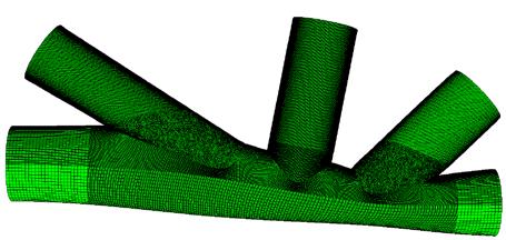
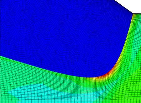
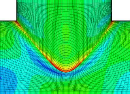
145 D.1.3 CALCULATION OF SCFs BALANCED AXIAL LOAD BRACE B CHORD LOC. A BRACE A LOAD TYPE/D.SHAPE 127

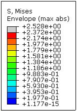
146 CHORD LOC. C BRACE C CHORD LOC. B 128

147 IN-PLANE BENDING (IPB) CHORD LOC. A BRACE A LOAD TYPE/D.SHAPE 129

148 IN-PLANE BENDING (IPB) CHORD LOC. B BRACE B LOAD TYPE/D.SHAPE 130

149 IN-PLANE BENDING (IPB) CHORD LOC. C BRACE C LOAD TYPE/D.SHAPE 131

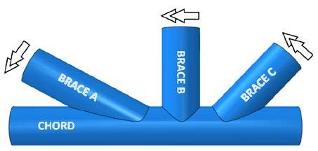
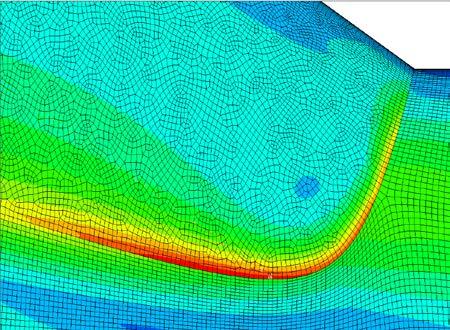
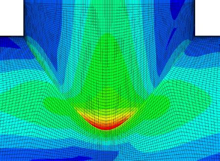
150 OUT-OF-PLANE BENDING (OPB) BRACE B CHORD LOC. A BRACE A LOAD TYPE/D.SHAPE 132

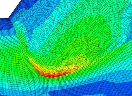
151 CHORD LOC. C BRACE C CHORD LOC. B 133

152 D.2 SCF CALCULATION OF TUBULAR JOINT 13 D.2.1 SECTION PROPERTIES Figure D-5: Definition of section properties of tubulars in tubular joint 13 Brace A: Wall thickness: Outer diameter: t A := d Ao := 16 mm 1200 mm Outer radius: r Ao d Ao := r 2 Ao = 600 mm Inner diameter: Inner radius: ( ) d Ai := d Ao 2 t A d Ai = mm d Ai r Ai := r 2 Ai = 584 mm Cross-sectional area: 2 2 A A := π r Ao r Ai A A = mm 2 Moment of inertia: π 4 4 I A := r 4 Ao r Ai I A = mm 4 Centre of the brace to mid-thickness of the brace: t A y A := r Ao y 2 A = 592 mm 134

153 Brace B: Wall thickness: Outer diameter: t B := d Bo := 14 mm 1200 mm Outer radius: r Bo d Bo := r 2 Bo = 600 mm Inner diameter: Inner radius: ( ) d Bi := d Bo 2 t B d Bi = mm d Bi r Bi := r 2 Bi = 586 mm Cross-sectional area: 2 2 A B := π r Bo r Bi A B = mm 2 Moment of inertia: π 4 4 I B := r 4 Bo r Bi I B = mm 4 Centre of the brace to mid-thickness of the brace: t B y B := r Bo y 2 B = 593 mm 135

154 Brace C: Wall thickness: Outer diameter: t C := d Co := 16 mm 1200 mm Outer radius: r Co d Co := r 2 Co = 600 mm Inner diameter: Inner radius: ( ) d Ci := d Co 2 t C d Ci = mm d Ci r Ci := r 2 Ci = 584 mm Cross-sectional area: 2 2 A C := π r Co r Ci A C = mm 2 Moment of inertia: π 4 4 I C := r 4 Co r Ci I C = mm 4 Centre of the brace to mid-thickness of the brace: t C y C := r Co y 2 C = 592 mm 136

155 Conversion of nominal stress into normal- and moment force: Figure D-6: Definition of normal forces in brace members of tubular joint 13 Nominal stress: σ nom := 1 MPa Normal force: N A := σ nom A A N A = N N Ax := N A cos( 46deg) N Ax = N N Ay := N A sin( 46deg) N Ay = N N B := σ nom A B N B = N N C := σ nom A C N C = N N Cx := N C cos( 46deg) N Cx = N N Cy := N C sin( 46deg) N Cy = N 137

156 Figure D-7: Definition of moment forces in brace members of tubular joint 13 Nominal stress: σ nom = 1 MPa Moment in-plane: ( ) σ nom I A M IP.A := M y IP.A = N mm A ( ) σ nom I B M IP.B := M y IP.B = N mm B ( ) σ nom I C M IP.C := M y IP.A = N mm C Moment out-of-plane: ( ) σ nom I A M OP.A := M y OP.A = N mm A ( ) σ nom I B M OP.B := M y OP.B = N mm B ( ) σ nom I C M OP.C := M y OP.A = N mm C 138

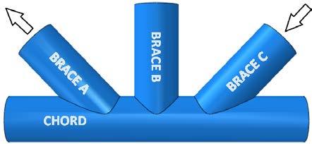
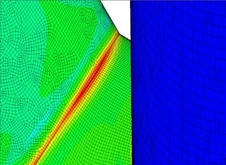
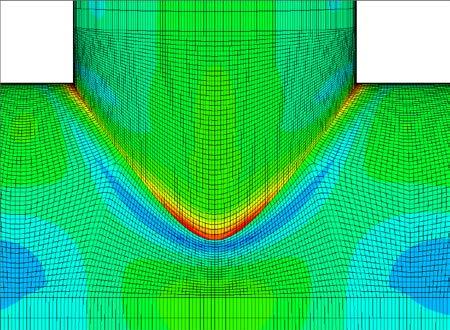
157 D.2.2 CALCULATION OF SCF BALANCED AXIAL LOAD BRACE B CHORD LOC. A BRACE A LOAD TYPE/D.SHAPE 139

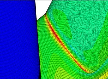
158 CHORD LOC. C BRACE C CHORD LOC. B 140

159 IN-PLANE BENDING (IPB) CHORD LOC. A BRACE A LOAD TYPE/D.SHAPE 141

160 IN-PLANE BENDING (IPB) CHORD LOC. B BRACE B LOAD TYPE/D.SHAPE 142

161 IN-PLANE BENDING (IPB) CHORD LOC. C BRACE C LOAD TYPE/D.SHAPE 143

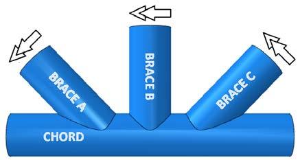
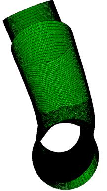
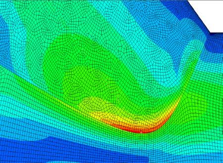
162 UNBALANCED OUT-OF-PLANE BENDING (OPB) CHORD LOC. A BRACE A LOAD TYPE/D.SHAPE 144

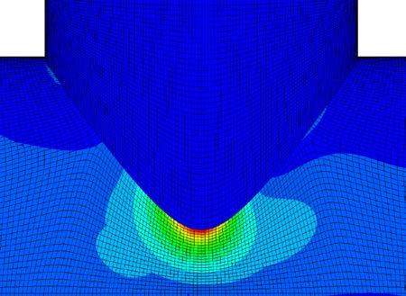
163 CHORD LOC. C BRACE C CHORD LOC. B BRACE B 145

164 APPENDIX E: FATIGUE LIFE CALCULATION FOR TUBULAR JOINTS 146

165 147

166 E.1 TUBULAR JOINT 9 Figure E-1: Illustration of normal and moment forces in brace members of tubular joint 9 Brace A: Wall thickness: Outer diameter: t A := d Ao := 16 mm 1200 mm Outer radius: r Ao d Ao := r 2 Ao = 600 mm Inner diameter: Inner radius: ( ) d Ai := d Ao 2 t A d Ai = mm d Ai r Ai := r 2 Ai = 584 mm Cross-sectional area: 2 2 A A := π r Ao r Ai A A = mm 2 Moment of inertia: π 4 4 I A := r 4 Ao r Ai I A = mm 4 Centre of the brace to mid-thickness of the brace: t A y A := r Ao y 2 A = 592 mm 148

167 Brace B: Wall thickness: Outer diameter: t B := d Bo := 14 mm 1200 mm Outer radius: r Bo d Bo := r 2 Bo = 600 mm Inner diameter: Inner radius: ( ) d Bi := d Bo 2 t B d Bi = mm d Bi r Bi := r 2 Bi = 586 mm Cross-sectional area: 2 2 A B := π r Bo r Bi A B = mm 2 Moment of inertia: π 4 4 I B := r 4 Bo r Bi I B = mm 4 Centre of the brace to mid-thickness of the brace: t B y B := r Bo y 2 B = 593 mm 149

168 Brace C: Wall thickness: Outer diameter: t C := d Co := 16 mm 1200 mm Outer radius: r Co d Co := r 2 Co = 600 mm Inner diameter: Inner radius: ( ) d Ci := d Co 2 t C d Ci = mm d Ci r Ci := r 2 Ci = 584 mm Cross-sectional area: 2 2 A C := π r Co r Ci A C = mm 2 Moment of inertia: π 4 4 I C := r 4 Co r Ci I C = mm 4 Centre of the brace to mid-thickness of the brace: t C y C := r Co y 2 C = 592 mm 150

169 Chord: Figure E-2: Illustration of normal and moment forces in chord member of tubular joint 9 Wall thickness: T := 40 mm Outer diameter: D o := 1248 mm Outer radius: r o D o := r 2 o = 624 mm Inner diameter: Inner radius: ( ) D i := D o 2 T D i = mm D i r i := r 2 i = 584 mm Cross-sectional area: 2 2 A := π r o r i A = mm 2 Moment of inertia: π 4 4 I := r 4 o r i I = mm 4 Centre of the brace to mid-thickness of the brace: T y := r o y = 604 mm z := y = 604 mm 2 151

170 E.1.1 HOT SPOT STRESS RANGE (HSSR) FOR Hs=1,5m Table E.1 Calculation of load range for Hs=1,5m in brace and chord member of tubular joint 9 LOAD RANGE Axial ( N x.i ) [N] IPB ( M y.i ) [Nmm] OPB ( M z..i ) [Nmm] Brace Location, i: A 49089, , ,51 B , ,98 C 40225, , ,17 Chord Location, i A 39551, , ,20 B 39551, , ,20 C 39551, , ,20 Axial: N x.i = (Max. Axial load Min. Axial load)[n] In-plane bending: M y.i = (Max. IPB load Min. IPB load)[nmm] Out-of-plane bending: M z.i = (Max. OPB load Min. OPB load)[nmm] Table E.2 Calculation of stress range for Hs=1,5m in brace and chord member of tubular joint 9 STRESS RANGE Axial ( σ x.i ) [MPa] IPB ( σ my.i ) [MPa] OPB ( σ mz.i ) [MPa] Brace Location, i: A 0,825 4,64E-03 0,057 B - 0,045 0,238 C 0,676 1,94E-03 0,035 Chord Location, i: A 0,261 0,019 1,179 B 0,261 0,019 1,179 C 0,261 0,019 1,179 Axial: σ x.i = N x.i /A i [MPa] In-plane bending: σ my.i = [( M y.i y i )/I y.i ][MPa] Out-of-plane bending: σ mz.i = [( M z.i y i )/I z.i ][MPa] 152

171 E CALCULATION OF HSSR DNV-RP-C203 Table E.3 Calculation of HSSR for Hs=1,5m according to SCF in DNV-RP-C203 [4] HSSR σ 1 σ 2 σ 3 σ 4 σ 5 σ 6 σ 7 σ 8 MAX HSSR σ b/c.i=1 Brace Location: A 1,237 1,123 1,070 1,108 1,216 1,330 1,383 1,345 1,383 B 0,093-0,643-1,002-0,774-0,093 0,643 1,002 0,774 1,002 C 1,359 1,297 1,269 1,291 1,351 1,413 1,441 1,419 1,441 Chord Location: A 0,475-2,190-3,305-2,217 0,437 3,102 4,217 3,129 4,217 B 0,889-2,879-4,455-2,918 0,833 4,600 6,177 4,640 6,177 C 0,723-1,681-2,691-1,716 0,674 3,078 4,088 3,133 4,088 Superposition of stresses in tubular joints; Where SCF SCF AC/AS SCF MIP SCF MOP Brace Location: A 1,487 2,341 2,765 B 2,589 2,073 4,201 C 2,005 2,219 2,492 Chord Location: A 1,750 0,975 3,189 B 3,304 1,478 4,508 C 2,681 1,315 2,

172 E CALCULATION OF HSSR ABAQUS/CAE Table E.4 Calculation of HSSR for Hs=1,5m according to SCF in ABAQUS/CAE [5] HSSR σ 1 σ 2 σ 3 σ 4 σ 5 σ 6 σ 7 σ 8 MAX HSSR σ b/c.i=1 Brace Location: A 1,868 1,727 1,663 1,715 1,852 1,993 2,057 2,005 2,057 B 0,101-0,874-1,337-1,017-0,101 0,874 1,337 1,017 1,337 C 1,607 1,504 1,459 1,498 1,599 1,703 1,748 1,708 1,748 Chord Location: A 0,557-3,852-5,690-3,879 0,519 4,928 6,766 4,955 6,766 B 1,263-6,278-9,416-6,314 1,212 8,753 11,891 8,788 11,891 C 0,902-5,238-7,796-5,274 0,850 6,990 9,549 7,270 9,549 Superposition of stresses in tubular joints; Where SCF SCF AC/AS SCF MIP SCF MOP Brace Location: A 2,255 1,693 3,464 B 2,670 2,253 5,608 C 2,372 1,952 4,190 Chord Location: A 2,065 0,885 5,281 B 4,749 1,335 9,034 C 3,363 1,379 7,

173 E.1.2 HOT SPOT STRESS RANGE (HSSR) FOR Hs=2,0m Table E.5 Calculation of load range for Hs=2,0m in brace and chord member of tubular joint 9 LOAD RANGE Axial ( N x.i ) [N] IPB ( M y.i ) [Nmm] OPB ( M z..i ) [Nmm] Brace Location, i: A 64039, , ,40 B , ,97 C 52930, , ,73 Chord Location, i A 49285, , ,00 B 49285, , ,00 C 49285, , ,00 Axial: N x.i = (Max. Axial load Min. Axial load)[n] In-plane bending: M y.i = (Max. IPB load Min. IPB load)[nmm] Out-of-plane bending: M z.i = (Max. OPB load Min. OPB load)[nmm] Table E.6 Calculation of stress range for Hs=2,0m in brace and chord member of tubular joint 9 STRESS RANGE Axial ( σ x.i ) [MPa] IPB ( σ my.i ) [MPa] OPB ( σ mz.i ) [MPa] Brace Location, i: A 1,081 5,307E-03 0,068 B - 0,059 0,314 C 0,889 1,427E-03 0,046 Chord Location, i: A 0,325 0,025 1,57 B 0,325 0,025 1,57 C 0,325 0,025 1,57 Axial: σ x.i = N x.i /A i [MPa] In-plane bending: σ my.i = [( M y.i y i )/I y.i ][MPa] Out-of-plane bending: σ mz.i = [( M z.i y i )/I z.i ][MPa] 155

174 E CALCULATION OF HSSR DNV-RP-C203 Table E.7 Calculation of HSSR for Hs=2,0m according to SCF in DNV-RP-C203 [4] HSSR σ 1 σ 2 σ 3 σ 4 σ 5 σ 6 σ 7 σ 8 MAX HSSR σ b/c.i=2 Brace Location: A 1,619 1,482 1,418 1,464 1,594 1,732 1,796 1,749 1,796 B 0,122-0,846-1,318-1,019-0,122 0,846 1,318 1,019 1,318 C 1,786 1,705 1,670 1,701 1,780 1,861 1,897 1,866 1,897 Chord Location: A 0,593-2,955-4,439-2,990 0,543 4,091 5,575 4,126 5,575 B 1,110-3,906-6,005-3,958 1,036 6,051 8,150 6,103 8,15 C 0,903-2,297-3,642-2,343 0,838 4,038 5,383 4,084 5,383 Superposition of stresses in tubular joints; Where SCF SCF AC/AS SCF MIP SCF MOP Brace Location: A 1,487 2,341 2,765 B 2,589 2,073 4,201 C 2,005 2,219 2,492 Chord Location: A 1,750 0,975 3,189 B 3,304 1,478 4,508 C 2,681 1,315 2,

175 E CALCULATION OF HSSR ABAQUS/CAE Brace Location: Table E.8 Calculation of HSSR for Hs=2,0m according to SCF in ABAQUS/CAE [5] HSSR σ 1 σ 2 σ 3 σ 4 σ 5 σ 6 σ 7 σ 8 MAX HSSR σ b/c.i=2 A 2,446 2,276 2,200 2,263 2,428 2,598 2,673 2,610 2,673 B - 0,133-1,150-1,760-1,339 0,133 1,150 1,760 1,339 1,760 C 2,112 1,977 1,919 1,973 2,107 2,243 2,300 2,247 2,300 Chord Location: A 0,695-5,175-7,621-5,210 0,646 6,516 8,962 6,551 8,962 B 1,575-8,464-12,642-8,511 1,509 11,548 15,725 11,595 15,725 C 1,126-7,048-10,454-7,097 1,058 9,232 12,638 9,280 12,638 Superposition of stresses in tubular joints; Where SCF SCF AC/AS SCF MIP SCF MOP Brace Location: A 2,255 1,693 3,464 B 2,670 2,253 5,608 C 2,372 1,952 4,190 Chord Location: A 2,065 0,885 5,281 B 4,749 1,335 9,034 C 3,363 1,379 7,

176 E.1.3 HOT SPOT STRESS RANGE (HSSR) FOR Hs=2,5m Table E.9 Calculation of load range for Hs=2,5m in brace and chord member of tubular joint 9 LOAD RANGE Axial ( N x.i ) [N] IPB ( M y.i ) [Nmm] OPB ( M z..i ) [Nmm] Brace Location, i: A 82754, , ,85 B , ,76 C 67845, , ,23 Chord Location, i A 63874, , ,00 B 63874, , ,00 C 63874, , ,00 Axial: N x.i = (Max. Axial load Min. Axial load)[n] In-plane bending: M y.i = (Max. IPB load Min. IPB load)[nmm] Out-of-plane bending: M z.i = (Max. OPB load Min. OPB load)[nmm] Table E.10 Calculation of stress range for Hs=2,5m in brace and chord member of tubular joint 9 STRESS RANGE Axial ( σ x.i ) [MPa] IPB ( σ my.i ) [MPa] OPB ( σ mz.i ) [MPa] Brace Location, i: A 1,39 7,08E-03 0,089 B - 0,075 0,402 C 1,14 2,046E-03 0,058 Chord Location, i: A 0,421 0,032 1,991 B 0,421 0,032 1,991 C 0,421 0,032 1,991 Axial: σ x.i = N x.i /A i [MPa] In-plane bending: σ my.i = [( M y.i y i )/I y.i ][MPa] Out-of-plane bending: σ mz.i = [( M z.i y i )/I z.i ][MPa] 158

177 E CALCULATION OF HSSR DNV-RP-C203 Table E.11 Calculation of HSSR for Hs=2,5m according to SCF in DNV-RP-C203 [4] HSSR σ 1 σ 2 σ 3 σ 4 σ 5 σ 6 σ 7 σ 8 MAX HSSR σ b/c.i=3 Brace Location: A 2,084 1,905 1,822 1,882 2,051 2,230 2,314 2,253 2,314 B 0,156-1,084-1,690-1,305-0,156 1,084 1,690 1,305 1,690 C 2,290 2,187 2,141 2,180 2,281 2,385 2,430 2,391 2,430 Chord Location: A 0,768-3,732-5,614-3,777 0,705 5,205 7,087 5,249 7,087 B 1,433-4,925-7,587-4,991 1,343 7,705 10,368 7,771 10,368 C 1,170-2,889-4,595-2,949 1,086 5,146 6,852 5,205 6,852 Superposition of stresses in tubular joints; Where SCF SCF AC/AS SCF MIP SCF MOP Brace Location: A 1,487 2,341 2,765 B 2,589 2,073 4,201 C 2,005 2,219 2,492 Chord Location: A 1,750 0,975 3,189 B 3,304 1,478 4,508 C 2,681 1,315 2,

178 E CALCULATION OF HSSR ABAQUS/CAE Brace Location: Table E.12 Calculation of HSSR for Hs=2,5m according to SCF in ABAQUS/CAE [5] HSSR σ 1 σ 2 σ 3 σ 4 σ 5 σ 6 σ 7 σ 8 MAX HSSR σ b/c.i=3 A 3,148 2,926 2,827 2,909 3,124 3,345 3,444 3,362 3,444 B - 0,170-1,475-2,256-1,715 0,170 1,475 2,256 1,715 2,256 C 2,708 2,535 2,461 2,529 2,700 2,873 2,947 2,879 2,947 Chord Location: A 0,901-6,545-9,648-6,590 0,837 8,283 11,386 8,328 11,386 B 2,041-10,693-15,992-10,753 1,956 14,690 19,989 14,750 19,989 C 1,459-8,910-13,230-8,972 1,371 11,740 16,060 11,802 16,060 Superposition of stresses in tubular joints; Where SCF SCF AC/AS SCF MIP SCF MOP Brace Location: A 2,255 1,693 3,464 B 2,670 2,253 5,608 C 2,372 1,952 4,190 Chord Location: A 2,065 0,885 5,281 B 4,749 1,335 9,034 C 3,363 1,379 7,

179 E.2 TUBULAR JOINT 13 Brace A: Figure E-3 Illustration of normal and moment forces in brace members of tubular joint 13 Wall thickness: Outer diameter: t A := d Ao := 16 mm 1200 mm Outer radius: r Ao d Ao := r 2 Ao = 600 mm Inner diameter: Inner radius: ( ) d Ai := d Ao 2 t A d Ai = mm d Ai r Ai := r 2 Ai = 584 mm Cross-sectional area: 2 2 A A := π r Ao r Ai A A = mm 2 Moment of inertia: π 4 4 I A := r 4 Ao r Ai I A = mm 4 Centre of the brace to mid-thickness of the brace: t A y A := r Ao y 2 A = 592 mm 161

180 Brace B: Wall thickness: Outer diameter: t B := d Bo := 14 mm 1200 mm Outer radius: r Bo d Bo := r 2 Bo = 600 mm Inner diameter: Inner radius: ( ) d Bi := d Bo 2 t B d Bi = mm d Bi r Bi := r 2 Bi = 586 mm Cross-sectional area: 2 2 A B := π r Bo r Bi A B = mm 2 Moment of inertia: π 4 4 I B := r 4 Bo r Bi I B = mm 4 Centre of the brace to mid-thickness of the brace: t B y B := r Bo y 2 B = 593 mm 162

181 Brace C: Wall thickness: Outer diameter: t C := d Co := 16 mm 1200 mm Outer radius: r Co d Co := r 2 Co = 600 mm Inner diameter: Inner radius: ( ) d Ci := d Co 2 t C d Ci = mm d Ci r Ci := r 2 Ci = 584 mm Cross-sectional area: 2 2 A C := π r Co r Ci A C = mm 2 Moment of inertia: π 4 4 I C := r 4 Co r Ci I C = mm 4 Centre of the brace to mid-thickness of the brace: t C y C := r Co y 2 C = 592 mm 163

182 Chord: Figure E-4: Illustration of normal and moment forces in chord member of tubular joint 13 Wall thickness: T := 40 mm Outer diameter: D o := 1248 mm Outer radius: r o D o := r 2 o = 624 mm Inner diameter: Inner radius: ( ) D i := D o 2 T D i = mm D i r i := r 2 i = 584 mm Cross-sectional area: 2 2 A := π r o r i A = mm 2 Moment of intertia: π 4 4 I := r 4 o r i I = mm 4 Centre of the brace to mid-thickness of the brace: T y := r o y = 604 mm z := y = 604 mm 2 164

183 E.2.1 HOT SPOT STRESS RANGE (HSSR) FOR Hs=1,5m Table D.13 Calculation of load range for Hs=1,5m in brace and chord member of tubular joint 13 LOAD RANGE Axial ( N x.i ) [N] IPB ( M y.i ) [Nmm] OPB ( M z..i ) [Nmm] Brace Location, i: A 40225, , ,17 B , ,53 C 54106, , ,03 Chord Location, i A 39551, , ,20 B 39551, , ,20 C 39551, , ,20 Axial: N x.i = (Max. Axial load Min. Axial load)[n] In-plane bending: M y.i = (Max. IPB load Min. IPB load)[nmm] Out-of-plane bending: M z.i = (Max. OPB load Min. OPB load)[nmm] Table E.14 Calculation of stress range for Hs=1,5m in brace and chord member of tubular joint 13 STRESS RANGE Axial ( σ x.i ) [MPa] IPB ( σ my.i ) [MPa] OPB ( σ mz.i ) [MPa] Brace Location, i: A 0,676 1,939E-03 0,035 B - 0,037 0,14 C 0,909 0,019 0,098 Chord Location, i: A 0,261 0,019 1,179 B 0,261 0,019 1,179 C 0,261 0,019 1,179 Axial: σ x.i = N x.i /A i [MPa] In-plane bending: σ my.i = [( M y.i y i )/I y.i ][MPa] Out-of-plane bending: σ mz.i = [( M z.i y i )/I z.i ][MPa] 165

184 E CALCULATION OF HSSR DNV-RP-C203 Table E.14 Calculation of HSSR for Hs=1,5m according to SCF in DNV-RP-C203 [4] HSSR σ 1 σ 2 σ 3 σ 4 σ 5 σ 6 σ 7 σ 8 MAX HSSR σ b/c.i=1 Brace Location: A 1,278 1,192 1,154 1,186 1,269 1,355 1,393 1,361 1,393 B 0,077-0,391-0,630-0,500-0,077 0,391 0,630 0,500 0,63 C 1,756 1,503 1,373 1,442 1,670 1,923 2,053 1,984 2,053 Chord Location: A 0,639-2,703-4,102-2,738 0,590 3,933 5,332 3,968 5,332 B 0,785-3,337-5,061-3,377 0,730 4,852 6,576 4,891 6,576 C 0,639-2,703-4,102-2,738 0,590 3,933 5,332 3,968 5,332 Superposition of stresses in tubular joints; Where SCF SCF AC/AS SCF MIP SCF MOP Brace Location: A 1,884 2,219 3,468 B 2,398 2,073 4,498 C 1,884 2,219 3,468 Chord Location: A 2,359 1,315 4,000 B 2,907 1,478 4,934 C 2,359 1,315 4,

185 E CALCUALTION OF HSSR ABAQUS/CAE Table E.15 Calculation of HSSR for Hs=1,5m according to SCF in ABAQUS/CAE [5] HSSR σ 1 σ 2 σ 3 σ 4 σ 5 σ 6 σ 7 σ 8 MAX HSSR σ b/c.i=1 Brace Location: A 1,479 1,375 1,329 1,369 1,472 1,576 1,622 1,582 1,622 B 0,084-0,496-0,785-0,614-0,084 0,496 0,785 0,614 0,785 C 2,022 1,719 1,571 1,666 1,948 2,251 2,398 2,303 2,398 Chord Location: A 0,905-5,311-7,901-5,348 0,854 7,071 9,661 7,107 9,661 B 1,265-6,578-9,841-6,613 1,215 9,058 12,322 9,094 12,322 C 0,915-5,294-7,882-5,331 0,863 7,072 9,659 7,109 9,659 Superposition of stresses in tubular joints; Where SCF SCF AC/AS SCF MIP SCF MOP Brace Location: A 2,183 1,913 4,240 B 2,637 2,251 5,604 C 2,183 1,913 4,213 Chord Location: A 3,376 1,362 7,446 B 4,760 1,334 9,397 C 3,411 1,375 7,

186 E.2.2 HOT SPOT STRESS RANGE (HSSR) FOR Hs=2,0m Table E.16 Calculation of load range for Hs=2,0m in brace and chord member of tubular joint 13 LOAD RANGE Axial ( N x.i ) [N] IPB ( M y.i ) [Nmm] OPB ( M z..i ) [Nmm] Brace Location, i: A 52930, , ,73 B , ,35 C 71569, , ,09 Chord Location, i A 49285, , ,00 B 49285, , ,00 C 49285, , ,00 Axial: N x.i = (Max. Axial load Min. Axial load)[n] In-plane bending: M y.i = (Max. IPB load Min. IPB load)[nmm] Out-of-plane bending: M z.i = (Max. OPB load Min. OPB load)[nmm] Table E.17 Calculation of stress range for Hs=2,0m in brace and chord member of tubular joint 13 STRESS RANGE Axial ( σ x.i ) [MPa] IPB ( σ my.i ) [MPa] OPB ( σ mz.i ) [MPa] Brace Location, i: A 0,889 1,427E-03 0,046 B - 0,049 0,185 C 1,203 0,025 0,129 Chord Location, i: A 0,325 0,025 1,57 B 0,325 0,025 1,57 C 0,325 0,025 1,57 Axial: σ x.i = N x.i /A i [MPa] In-plane bending: σ my.i = [( M y.i y i )/I y.i ][MPa] Out-of-plane bending: σ mz.i = [( M z.i y i )/I z.i ][MPa] 168

187 E CALCULATION OF HSSR DNV-RP-C203 Table E.17 Calculation of HSSR for Hs=2,0m according to SCF in DNV-RP-C203 [4] HSSR σ 1 σ 2 σ 3 σ 4 σ 5 σ 6 σ 7 σ 8 MAX HSSR σ b/c.i=2 Brace Location: A 1,679 1,566 1,518 1,562 1,672 1,785 1,834 1,790 1,834 B 0,101-0,517-0,832-0,660-0,101 0,517 0,832 0,660 0,832 C 2,322 1,990 1,819 1,910 2,209 2,542 2,712 2,621 2,712 Chord Location: A 0,799-3,652-5,514-3,698 0,733 5,183 7,046 5,230 7,046 B 0,981-4,508-6,803-4,560 0,907 6,395 8,690 6,447 8,69 C 0,799-3,652-5,514-3,698 0,733 5,183 7,046 5,230 7,046 Superposition of stresses in tubular joints; Where SCF SCF AC/AS SCF MIP SCF MOP Brace Location: A 1,884 2,219 3,468 B 2,398 2,073 4,498 C 1,884 2,219 3,468 Chord Location: A 2,359 1,315 4,000 B 2,907 1,478 4,934 C 2,359 1,315 4,

188 E CALCULATION OF HSSR ABAQUS/CAE Table E.18 Calculation of HSSR for Hs=2,0m according to SCF in ABAQUS/CAE [5] HSSR σ 1 σ 2 σ 3 σ 4 σ 5 σ 6 σ 7 σ 8 MAX HSSR σ b/c.i=2 Brace Location: A 1,944 1,807 1,748 1,803 1,939 2,076 2,135 2,080 2,135 B 0,110-0,655-1,037-0,811-0,110 0,655 1,037 0,811 1,037 C 2,674 2,276 2,083 2,207 2,577 2,974 3,168 3,043 3,168 Chord Location: A 1,130-7,146-10,594-7,194 1,062 9,338 12,786 9,386 12,786 B 1,579-8,863-13,208-8,910 1,512 11,954 16,299 12,001 16,299 C 1,142-7,125-10,569-7,173 1,073 9,340 12,784 9,388 12,784 Superposition of stresses in tubular joints; Where SCF SCF AC/AS SCF MIP SCF MOP Brace Location: A 2,183 1,913 4,240 B 2,637 2,251 5,604 C 2,183 1,913 4,213 Chord Location: A 3,376 1,362 7,446 B 4,760 1,334 9,397 C 3,411 1,375 7,

189 E.2.3 HOT SPOT STRESS RANGE (HSSR) FOR Hs=2,5m Table E.19 Calculation of load range for Hs=2,5m in brace and chord member of tubular joint 13 LOAD RANGE Axial ( N x.i ) [N] IPB ( M y.i ) [Nmm] OPB ( M z..i ) [Nmm] Brace Location, i: A 67845, , ,23 B , ,56 C 91313, , ,80 Chord Location, i A 63874, , ,00 B 63874, , ,00 C 63874, , ,00 Axial: N x.i = (Max. Axial load Min. Axial load)[n] In-plane bending: M y.i = (Max. IPB load Min. IPB load)[nmm] Out-of-plane bending: M z.i = (Max. OPB load Min. OPB load)[nmm] Table E.20 Calculation of stress range for Hs=2,5m in brace and chord member of tubular joint 13 STRESS RANGE Axial ( σ x.i ) [MPa] IPB ( σ my.i ) [MPa] OPB ( σ mz.i ) [MPa] Brace Location, i: A 1,14 2,046E-03 0,058 B - 0,063 0,236 C 1,534 0,033 0,165 Chord Location, i: A 0,421 0,032 1,991 B 0,421 0,032 1,991 C 0,421 0,032 1,991 Axial: σ x.i = N x.i /A i [MPa] In-plane bending: σ my.i = [( M y.i y i )/I y.i ][MPa] Out-of-plane bending: σ mz.i = [( M z.i y i )/I z.i ][MPa] 171

190 E CALCULATION OF HSSR DNV-RP-C203 Table E.21 Calculation of HSSR for Hs=2,5m according to SCF in DNV-RP-C203 [4] HSSR σ 1 σ 2 σ 3 σ 4 σ 5 σ 6 σ 7 σ 8 MAX HSSR σ b/c.i=3 Brace Location: A 2,152 2,009 1,946 2,002 2,143 2,287 2,349 2,293 2,349 B 0,130-0,660-1,063-0,844-0,130 0,660 1,063 0,844 1,063 C 2,963 2,536 2,317 2,434 2,818 3,245 3,464 3,347 3,464 Chord Location: A 1,034-4,611-6,973-4,670 0,951 6,596 8,958 6,665 8,958 B 1,270-5,691-8,603-5,758 1,176 8,138 11,049 8,204 11,049 C 1,034-4,611-6,973-4,670 0,951 6,596 8,958 6,655 8,958 Superposition of stresses in tubular joints; Where SCF SCF AC/AS SCF MIP SCF MOP Brace Location: A 1,884 2,219 3,468 B 2,398 2,073 4,498 C 1,884 2,219 3,468 Chord Location: A 2,359 1,315 4,000 B 2,907 1,478 4,934 C 2,359 1,315 4,

191 E CALCULATION OF HSSR ABAQUS/CAE Table E.22 Calculation of HSSR for Hs=2,5m according to SCF in ABAQUS/CAE [5] HSSR σ 1 σ 2 σ 3 σ 4 σ 5 σ 6 σ 7 σ 8 MAX HSSR σ b/c.i=3 Brace Location: A 2,493 2,317 2,242 2,312 2,485 2,660 2,735 2,665 2,735 B 0,141-0,836-1,324-1,036-0,141 0,836 1,324 1,036 1,324 C 3,412 2,901 2,653 2,813 3,287 3,798 4,046 3,886 4,046 Chord Location: A 1,464-9,034-13,408-9,095 1,377 11,875 16,249 11,936 16,249 B - - 2,045 11,200-16,711 11,260 1,961 15,205 20,717 15,265 20,717 C 1,479-9,006-13,375-9,068 1,392 11,877 16,246 11,939 16,246 Superposition of stresses in tubular joints; Where SCF SCF AC/AS SCF MIP SCF MOP Brace Location: A 2,183 1,913 4,240 B 2,637 2,251 5,604 C 2,183 1,913 4,213 Chord Location: A 3,376 1,362 7,446 B 4,760 1,334 9,397 C 3,411 1,375 7,

192 E.3 FATIGUE LIFE E.3.1 TUBULAR JOINT 9 Table E.23 Calculation of wave cycles (per year) for each significant wave height, Hs [m] Peak wave period of each Hs: 9 s Wave duration: 3 Hours 1 year = 365 days Total wave duration [s] Total wave cycles [per day] Total wave cycles [per year] Hs [m] Wave action [#] Wave duration [s] 1, ,31E+06 2, ,31E+06 2, ,76E+05 Total wave duration [s] = Wave duration[s] Wave action Total wave cycles [per day] = Total wave duration [s]/peak wave period[s] Total wave cycles [per year] = Total wave cycles [per day] 365 days E FATIGUE LIFE: DNV-RP-C203 Table E.24 Calculation of cumulative damage in brace member for each Hs at location A, B and C of tubular joint 9 Hs [m] 1,50 2,00 Location Max HSSR BRACE Number of reg. cycles [n] Number of predicted cycles [N] n/n A 1,383 1,314E+06 7,98E+14 1,65E-09 B 1,002 1,314E+06 4,00E+15 3,29E-10 C 1,441 8,760E+05 1,94E+11 4,51E-06 A 1,796 1,314E+06 2,16E+14 6,08E-09 B 1,318 1,314E+06 1,01E+15 1,29E-09 C 1,897 8,760E+05 8,51E+10 1,03E-05 A 2,314 1,314E+06 6,08E+13 2,16E-08 2,50 B 1,690 1,314E+06 2,93E+14 4,49E-09 C 2,430 8,760E+05 4,05E+10 2,16E-05 Max HSSR: Reference is made to Table E.3, Table E.7 and Table E.11 Number of re. cycles[n]: Reference is made to Table E.22 Number of predicted cycles[n]: Reference is made to Section 3.4.1, Eq (3.1) 174

193 BRACE Location: Table E.25 Calculation of fatigue life in brace members of tubular joint 9 Cumulative damage [D] FATIGUE LIFE [Years] Fatigue Life (DFF=1) Fatigue Life (DFF=3) A 2,93E-08 B 6,11E-09 C 3,65E-05 k=3 Cumulative damage, D = n i N i i=1 Fatigue life, FL = [1/(D DFF)[Years] Table E.26 Calculation of cumulative damage in chord member for each Hs at location A, B and C of tubular joint 9 Hs [m] 1,50 2,00 Location Max HSSR CHORD Number of reg. cycles [n] Number of predicted cycles [N] n/n A 4,217 1,31E+06 2,29E+12 5,74E-07 B 6,177 1,31E+06 3,40E+11 3,87E-06 C 4,088 8,76E+05 7,19E+09 1,22E-04 A 5,575 1,31E+06 5,67E+11 2,32E-06 B 8,15 1,31E+06 8,49E+10 1,55E-05 C 5,383 8,76E+05 3,15E+09 2,78E-04 A 7,087 1,31E+06 1,71E+11 7,69E-06 2,50 B 10,368 1,31E+06 2,55E+10 5,15E-05 C 6,852 8,76E+05 1,53E+09 5,74E-04 Max HSSR: Reference is made to Table E.3, Table E.7 and Table E.11 Number of re. cycles[n]: Reference is made to Table E.22 Number of predicted cycles[n]: Reference is made to Section 3.4.1, Eq (3.1) 175

194 CHORD Location: Table E.27 Calculation of fatigue life in chord member of tubular joint 9 Cumulative damage [D] FATIGUE LIFE [Years] Fatigue Life (DFF=1) Fatigue Life (DFF=3) A 1,06E-05 B 7,09E-05 C 9,74E k=3 Cumulative damage, D = n i N i i=1 Fatigue life, FL = [1/(D DFF)[Years] E FATIGUE LIFE: ABAQUS/CAE Table E.28 Calculation of cumulative damage in brace member for each Hs at location at A, B and C of tubular joint 9 Hs [m] 1,50 2,00 Location Max HSSR BRACE Number of reg. cycles [n] Number of predicted cycles [N] n/n A 2,057 1,314E+06 1,10E+14 1,20E-08 B 1,337 1,314E+06 9,45E+14 1,39E-09 C 1,748 8,760E+05 1,09E+11 8,06E-06 A 2,673 1,314E+06 2,96E+13 4,44E-08 B 1,760 1,314E+06 2,39E+14 5,50E-09 C 2,256 8,760E+05 5,06E+10 1,73E-05 A 3,444 1,314E+06 8,33E+12 1,58E-07 2,50 B 2,256 1,314E+06 6,91E+13 1,90E-08 C 2,947 8,760E+05 2,27E+10 3,86E-05 Max HSSR: Reference is made to Table E.4, Table E.8 and Table E.12 Number of re. cycles[n]: Reference is made to Table E.22 Number of predicted cycles[n]: Reference is made to Section 3.4.1, Eq (3.1) 176

195 BRACE Location: Table E.29 Calculation of fatigue life in brace members of tubular joint 9 Cumulative damage [D] FATIGUE LIFE [Years] Fatigue Life (DFF=1) Fatigue Life (DFF=3) A 2,14E-07 B 2,59E-08 C 6,40E-05 k=3 Cumulative damage, D = n i N i i=1 Fatigue life, FL = [1/(D DFF)[Years] Table E.30 Calculation of cumulative damage in chord member for each Hs at location A, B and C of tubular joint 9 Hs [m] 1,50 2,00 Location Max HSSR CHORD Number of reg. cycles [n] Number of predicted cycles [N] n/n A 6,766 1,31E+06 2,15E+11 6,10E-06 B 11,891 1,31E+06 1,28E+10 1,02E-04 C 9,549 8,76E+05 5,64E+08 1,55E-03 A 8,962 1,31E+06 5,28E+10 2,49E-05 B 15,725 1,31E+06 3,18E+09 4,14E-04 C 12,638 8,76E+05 2,43E+08 3,60E-03 A 11,386 1,31E+06 1,60E+10 8,23E-05 2,50 B 19,989 1,31E+06 9,57E+08 1,37E-03 C 16,060 8,76E+05 1,19E+08 7,39E-03 Max HSSR: Reference is made to Table E.4, Table E.8 and Table E.12 Number of re. cycles[n]: Reference is made to Table E.22 Number of predicted cycles[n]: Reference is made to Section 3.4.1, Eq (3.1) 177

196 CHORD Location: Table E.31 Calculation of fatigue life in chord member of tubular joint 9 Cumulative damage [D] FATIGUE LIFE [Years] Fatigue Life (DFF=1) Fatigue Life (DFF=3) A 1,13E-04 B 1,89E-03 C 1,25E k=3 Cumulative damage, D = n i N i i=1 Fatigue life, FL = [1/(D DFF)[Years] E.3.2 TUBULAR JOINT 13 Table E.32 Calculation of wave cycles (per year) for each significant wave height, Hs [m] Peak wave period of each Hs: 9 s Wave duration: 3 Hours 1 year = 365 days Total wave duration [s] Total wave cycles [per day] Total wave cycles [per year] Hs [m] Wave action [#] Wave duration [s] 1, ,31E+06 2, ,31E+06 2, ,76E+05 Total wave duration [s] = Wave duration[s] Wave action Total wave cycles [per day] = Total wave duration [s]/peak wave period[s] Total wave cycles [per year] = Total wave cycles [per day] 365 days 178

197 E FATIGUE LIFE: DNV-RP-C203 Table E.33 Calculation of cumulative damage in brace member for each Hs at location A, B and C of tubular joint 13 Hs [m] 1,50 2,00 Location Max HSSR BRACE Number of reg. cycles [n] Number of predicted cycles [N] n/n A 1,393 1,31E+06 7,70E+14 1,71E-09 B 0,630 1,31E+06 4,07E+16 3,23E-11 C 2,053 8,76E+05 6,71E+10 1,31E-05 A 1,834 1,31E+06 1,95E+14 6,75E-09 B 0,832 1,31E+06 1,01E+16 1,30E-10 C 2,712 8,76E+05 2,91E+10 3,01E-05 A 2,349 1,31E+06 5,64E+13 2,33E-08 2,50 B 1,063 1,31E+06 2,97E+15 4,42E-10 C 3,464 8,76E+05 1,40E+10 6,27E-05 Max HSSR: Reference is made to Table E.14, Table E.17 and Table E.21 Number of re. cycles[n]: Reference is made to Table E.31 Number of predicted cycles[n]: Reference is made to Section 3.4.1, Eq (3.1) BRACE Location: Table E.34 Calculation of fatigue life in brace members of tubular joint 13 Cumulative damage [D] FATIGUE LIFE [Years] Fatigue Life (DFF=1) Fatigue Life (DFF=3) A 3,17E-08 B 6,04E-10 C 1,06E-04 k=3 Cumulative damage, D = n i N i i=1 Fatigue life, FL = [1/(D DFF)[Years] 179

198 Table E.35 Calculation of cumulative damage in chord member for each Hs at location A, B and C of tubular joint 13 Hs [m] 1,50 2,00 Location Max HSSR CHORD Number of reg. cycles [n] Number of predicted cycles [N] n/n A 5,332 1,31E+06 7,09E+11 1,85E-06 B 6,576 1,31E+06 2,48E+11 5,29E-06 C 5,332 8,76E+05 3,24E+09 2,70E-04 A 7,046 1,31E+06 1,76E+11 7,47E-06 B 8,69 1,31E+06 6,16E+10 2,13E-05 C 7,046 8,76E+05 1,40E+09 6,24E-04 A 8,958 1,31E+06 5,29E+10 2,48E-05 2,50 B 11,049 1,31E+06 1,85E+10 7,09E-05 C 8,958 8,76E+05 6,83E+08 1,28E-03 Max HSSR: Reference is made to Table E.14, Table E.17 and Table E.21 Number of re. cycles[n]: Reference is made to Table E.31 Number of predicted cycles[n]: Reference is made to Section 3.4.1, Eq (3.1) CHORD Location: Table E.36 Calculation of fatigue life in chord member of tubular joint 13 Cumulative damage [D] FATIGUE LIFE [Years] Fatigue Life (DFF=1) Fatigue Life (DFF=3) A 3,41E-05 B 9,75E-05 C 2,18E k=3 Cumulative damage, D = n i N i i=1 Fatigue life, FL = [1/(D DFF)[Years] 180

199 E FATIGUE LIFE: ABAQUS/CAE Table E.37 Calculation of cumulative damage in brace member for each Hs at location A, B and C Hs [m] 1,50 2,00 Location Max HSSR BRACE Number of reg. cycles [n] Number of predicted cycles [N] n/n A 1,622 1,31E+06 3,60E+14 3,65E-09 B 0,785 1,31E+06 1,35E+16 9,70E-11 C 2,398 8,76E+05 4,21E+10 2,08E-05 A 2,135 1,31E+06 9,10E+13 1,44E-08 B 1,037 1,31E+06 3,37E+15 3,90E-10 C 3,168 8,76E+05 1,83E+10 4,80E-05 A 2,735 1,31E+06 2,64E+13 4,98E-08 2,50 B 1,324 1,31E+06 9,92E+14 1,32E-09 C 4,046 8,76E+05 8,77E+09 9,99E-05 Max HSSR: Reference is made to Table E.15, Table E.18 and Table E.22 Number of re. cycles[n]: Reference is made to Table E.31 Number of predicted cycles[n]: Reference is made to Section 3.4.1, Eq (3.1) BRACE Location: Table E.37 Calculation of fatigue life in brace member of tubular joint 13 Cumulative damage [D] FATIGUE LIFE [Years] Fatigue Life (DFF=1) Fatigue Life (DFF=3) A 6,79E-08 B 1,81E-09 C 1,69E-04 k=3 Cumulative damage, D = n i N i i=1 Fatigue life, FL = [1/(D DFF)[Years] 181

200 Table E.39 Calculation of cumulative damage in chord member for each at location A, B and C of tubular joint 13 Hs [m] 1,50 2,00 Location Max HSSR CHORD Number of reg. cycles [n] Number of predicted cycles [N] n/n A 9,661 1,31E+06 3,63E+10 3,62E-05 B 12,322 1,31E+06 1,08E+10 1,22E-04 C 9,659 8,76E+05 5,45E+08 1,61E-03 A 12,786 1,31E+06 8,94E+09 1,47E-04 B 13,222 1,31E+06 7,56E+09 1,74E-04 C 12,784 8,76E+05 2,35E+08 3,73E-03 A 16,249 1,31E+06 2,70E+09 4,87E-04 2,50 B 20,717 1,31E+06 8,00E+08 1,64E-03 C 16,246 8,76E+05 1,15E+08 7,65E-03 Max HSSR: Reference is made to Table E.15, Table E.18 and Table E.22 Number of re. cycles[n]: Reference is made to Table E.31 Number of predicted cycles[n]: Reference is made to Section 3.4.1, Eq (3.1) CHORD Location: Table E.39 Calculation of fatigue life in chord member of tubular joint 13 Cumulative damage [D] FATIGUE LIFE [Years] Fatigue Life (DFF=1) Fatigue Life (DFF=3) A 6,71E-04 B 1,94E-03 C 1,30E k=3 Cumulative damage, D = n i N i i=1 Fatigue life, FL = [1/(D DFF)[Years] 182

201 APPENDIX F: VERIFICATION OF THE FE MODEL AND ANALYSIS PROCEDURE 183

202 184

203 F.1 CALCULATION OF SCF DNV-RP-C203 F.1.1 T-JOINT Chord: Outer diameter: Figure F-1: Definition of geometrical parameters of T-joint D := 508 mm Thickness: Length: T := L := mm 1575mm Brace: Outer diameter: d := mm Thickness: t := mm Angle in degree: Θ := 90 Gap: g := 0mm Non-dimensional geometric parameters: d β := β = 0.8 D τ γ t := τ = 0.99 T D := γ = T L α := 2 D g ζ := D α = 6.2 ζ = 0 185

204 Check the validity range to utilize SCF equations given in Table B-5 ref. [4]: Chord: α check := "OK" if α 4 α 40 "NOT OK" otherwise α check = "OK" γ check := "OK" if γ 8 γ 32 "NOT OK" otherwise γ check = "OK" 0.6 β ζ check := "OK" if ζ ζ 1.0 sin( Θ deg) "NOT OK" otherwise ζ check = "OK" Brace: β check := "OK" if β 0.2 β 1.0 "NOT OK" otherwise β check = "OK" τ check := "OK" if τ 0.2 τ 1.0 "NOT OK" otherwise τ check = "OK" Θ check := "OK" if Θ 20 Θ 90 "NOT OK" otherwise Θ check = "OK" 186

205 Axial load: Figure F-2: Illustration of load type: Axial load of T-joint Short chord correction factors (α <12): F β 0.56 β := 0.02 exp 0.21 γ α 2.5 = 0.69 Chord saddle: ( ) γ 0.23 ( ) ( ) F β 1.8 γ := exp 0.49 γ α 1.8 = SCF CS := γ τ ( β 0.52) 2 ( sin( Θ deg) ) 1.6 F1 SCF CS = Chord crown: SCF CC := γ 0.2 τ ( β 0.65) 2 Brace saddle: SCF CC = τ β [ ( 0.25α) 3] ( sin( Θ deg) ) SCF BS 1.3 γ τ 0.52 α β α := + ( β 0.96) ( sin( Θ deg) ) [ ( )] Brace crown: SCF BS = ( ) SCF BC := 3 + γ exp( 4β) β β τ ( 0.1α 1.2) SCF BC =

206 In-plane bending: Figure F-3: Illustration of load type: In-plane bending (IPB) of T-joint Chord crown: SCF IPBcc := 1.45 β τ 0.85 γ [ 1 ( 0.68 β) ] ( sin( Θ deg) ) 0.7 SCF IPBcc = Brace crown: SCF IPBbc β τ β γ [ ( )] [( 0.06 γ ) 1.16] := + ( sin( Θ deg) ) SCF IPBbc =

207 Out-of-plane bending: Figure F-4: Illustration of load type: Out-of-Plane bending (OPB) of T-joint Chord saddle: SCF OPBcs := γ τ ( ) β β 3 ( sin( Θ deg) ) 1.6 F3 SCF OPBcs = Brace saddle: ( ) SCFOPBcs SCF OPBbs := τ γ β β 4 SCF OPBbs =

208 F.1.2 K-JOINT Chord: Outer diameter: Figure F-5: Definition of geometrical parameters of K-joint D := 508 mm Thickness: Length: T := L := mm mm Brace A: Outer diamater: d A := 254 mm Thickness: Angle in degree: Gap: Brace B: Outer diamater: Thickness: Angle in degree: Gap: t A := mm Θ A := 45 g AB := 76.2mm d B := t B := 254 mm mm Θ B := 45 g BA := 76.2mm Non-dimensional geometric parameters: β A d A d B := β D A = 0.5 β B := β D A = 0.5 τ A t A t B := τ T A = 1 τ B := τ T B = 1 γ D := γ = T L α := 2 α = 12.6 D g AB g BA ζ AB := ζ D AB = 0.15 ζ BA := ζ D BA =

209 Check the validity range to utilize SCF equations given in Table B-5 ref. [4]: ( ) β min := min β A, β B β min = 0.5 ( ) β max := max β A, β B β max = 0.5 ( ) Θ min := min Θ A, Θ B Θ min = 45 ( ) Θ max := max Θ A, Θ B Θ max = 45 Chord: α check := "OK" if α 4 α 40 "NOT OK" otherwise α check = "OK" γ check := "OK" if γ 8 γ 32 "NOT OK" otherwise γ check = "OK" 0.6 β max ζ AB.check := "OK" if ζ AB ζ sin Θ max deg AB 1.0 "NOT OK" otherwise ( ) ζ AB.check = "OK" 0.6 β max ζ BA.check := "OK" if ζ BA ζ sin Θ max deg BA 1.0 "NOT OK" otherwise ( ) ζ BA.check = "OK" 191

210 Brace A: β A.check := "OK" if β A 0.2 β A 1.0 "NOT OK" otherwise β A.check = "OK" τ A.check := "OK" if τ A 0.2 τ A 1.0 "NOT OK" otherwise τ A.check = "OK" Θ A.check := "OK" if Θ A 20 Θ A 90 "NOT OK" otherwise Θ A.check = "OK" Brace B: β B.check := "OK" if β B 0.2 β B 1.0 "NOT OK" otherwise β B.check = "OK" τ B.check := "OK" if τ B 0.2 τ B 1.0 "NOT OK" otherwise τ B.check = "OK" Θ B.check := "OK" if Θ B 20 Θ B 90 "NOT OK" otherwise Θ B.check = "OK" 192

211 Balanced axial load: Chord: Figure F-6: Illustration of load type: Balanced axial load of K-joint SCF ca := τ A γ 0.67 β A β A sin Θ A deg ( ) ( ) ( ) sin Θ max deg sin Θ min deg 0.3 β max 0.38 SCF chorda := SCF ca β β A atan 8 ζ AB min ( ) 0.3 = SCF chorda = SCF cb := τ B γ 0.67 β B β B sin Θ B deg 0.3 ( ) ( ) ( ) sin Θ max deg sin Θ min deg ( ) β max 0.38 SCF chordb := SCF cb β β B atan 8 ζ AB min 0.3 = SCF chordb =

212 Brace: For gap joints: C := 0 ( ) atan ( 14 ζ AB ) + ( 4.2 β A ) A := sin Θ max Θ min C β 1.5 A γ τ A 0.25 SCF bracea β A τ 0.14 := + A sin Θ A deg + A SCF bracea = ( ( )) 0.7 SCF chorda ( ) atan ( 14 ζ AB ) + ( 4.2 β A ) B := sin Θ max Θ min C β 1.5 B γ τ B 0.25 SCF braceb β B τ 0.14 := + B sin Θ B deg + B SCF braceb = ( ( )) 0.7 SCF chordb 194

213 Unbalanced in plane bending: Figure F-7: Illustration of load type: Unbalanced In-Plane bending of K-joint Chord crown: β A SCF MIPchordA 1.45 β A τ A γ := SCF MIPchordA = β B SCF MIPchordB 1.45 β B τ B γ := ( ) ( sin( Θ A deg) ) 0.7 ( ) ( sin( Θ B deg) ) 0.7 SCF MIPchordB = Brace crown: ( ) β A SCF MIPbraceA β A τ A γ := + sin Θ A deg SCF MIPbraceA = 3.66 ( ) ( ( )) β B SCF MIPbraceB β B τ B γ := + sin Θ B deg SCF MIPbraceB = 3.66 ( ( )) [( 0.06 γ ) 1.16] [( 0.06 γ ) 1.16] 195

214 Unbalanced out-of-plane bending: Figure F-8: Illustration of load type: Unbalanced Out-of-Plane bending of K-joint Chord saddle: 3 SCF MOPcA := γ τ A β A β A ( sin( Θ A deg) ) 1.6 = SCF MOPcB := γ τ B β B β B ( sin( Θ B deg) ) 1.6 = Chord saddle SCF adjacent to diagonal brace A: ( ) ζ AB sin Θ A deg X AB := 1 + = β A SCF MOPchordA := SCF MOPcA β B γ ( ) 0.5 exp( 0.8 X AB ) ( ) 0.5 exp( 0.8 ) SCF MOPcB β A γ X AB 2.05 β max exp 1.3 X AB... ( ) SCF MOPchordA = Brace A saddle SCF: ( ) SCF MOPbraceA := τ A γ β A β A SCF MOPchordA SCF MOPbraceA =

215 Chord saddle SCF adjacent to diagonal brace B: ( ) ζ AB sin Θ B deg X BA := 1 + = β B SCF MOPchordB := SCF MOPcA β A γ ( ) 0.5 exp( 0.8 X BA ) ( ) 0.5 exp( 0.8 ) SCF MOPcB β B γ X BA 2.05 β max exp 1.3 X BA... ( ) SCF MOPchordA = Brace B saddle SCF: ( ) SCF MOPbraceB := τ B γ β B β B SCF MOPchordB SCF MOPbraceB =

216 F.2 CALCULATION OF SCF FEA (ABAQUS/CAE) F.2.1 T-JOINT Section properties of tubular: Figure F-9: Definition of section properties of T-joint Brace: Outer radius: r o d := r 2 o = mm Inner diameter: d i := d ( 2 t) d i = mm Inner radius: d i r i := r 2 i = mm Cross-sectional area: 2 2 A := π r o r i A = mm 2 Moment of inertia: π 4 4 I := r 4 o r i I = mm 4 Centre of the brace to mid-thickness of the brace: t y := r o y = mm 2 198

217 Conversion of nominal stress into normal- and moment force: Nominal stress: σ nom := 1 MPa Axial force: N := σ nom A N = N In-plane bending: ( ) σ nom I M IPB := M y IPB = N mm Out-of-plane bending: ( ) σ nom I M OPB := M y OPB = N mm (a) Geometry of T-joint (b) Geometry of analysis model (T-joint) with BC and load assignment Figure F-10: Verification FE model (T-joint) 199

218 AXIAL BRACE CROWN BRACE SADDLE CHORD CROWN CHORD SADDLE LOAD TYPE/D.SHAPE 200

219 IN-PLANE BENDING BRACE CROWN CHORD CROWN LOAD TYPE/D.SHAPE 201

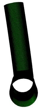
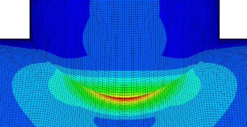
220 OUT-OF-PLANE BENDING BRACE SADDLE CHORD SADDLE LOAD TYPE/D.SHAPE 202

221 F.2.2 K-JOINT Section properties of tubulars: Brace A/B: Figure F-11: Definition of section properties of K-joint Outer radius: Inner diameter: Inner radius: d A r Ao := r 2 Ao = 127 mm ( ) d Ai := d A 2 t A d Ai = mm d Ai r Ai := r 2 Ai = mm Cross-sectional area: 2 2 A A := π r Ao r Ai A A = mm 2 Moment of inertia: π 4 4 I A := r 4 Ao r Ai I A = mm 4 Centre of the brace to mid-thickness of the brace: t A y A := r Ao y 2 A = mm 203

222 Conversion of nominal stress into normal- and moment force: Nominal stress: σ nom := 1 MPa Axial force: N A := σ nom A A N A = N N B := σ nom A B N B = N In-plane bending: ( ) σ nom I A M IPB.A := M y IPB.A = N mm A ( ) σ nom I B M IPB.B := M y IPB.B = N mm B Out-of-plane bending: ( ) σ nom I A M OPB.A := M y OPB.A = N mm A ( ) σ nom I B M OPB.B := M y OPB.B = N mm B 204

223 (a) Geometry of KT-joint (b) Geometry of analysis model (KT-joint) with BC and load assignment Figure F-12: Verification FE model (KT-joint) 205

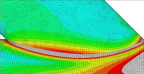
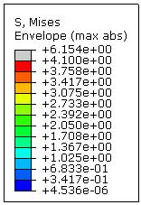
224 BALANCED AXIAL BRACE CROWN BRACE SADDLE CHORD CROWN CHORD SADDLE LOAD TYPE/D.SHAPE 206

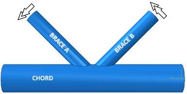
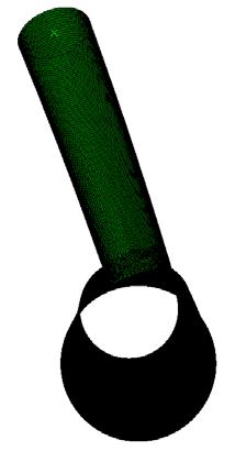
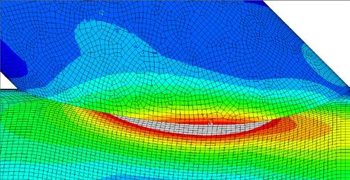
225 UNBALANCED OUT-OF-PLANE BENDING BRACE SADDLE CHORD SADDLE LOAD TYPE/D.SHAPE 207