Cfd Analysis Of A Uni-directional Impulse Turbine For Wave Energy Conversion

Transcription

1 University of Central Florida Electronic Theses and Dissertations Masters Thesis (Open Access) Cfd Analysis Of A Uni-directional Impulse Turbine For Wave Energy Conversion 2011 Carlos Alberto Velez University of Central Florida Find similar works at: University of Central Florida Libraries Part of the Aerodynamics and Fluid Mechanics Commons STARS Citation Velez, Carlos Alberto, "Cfd Analysis Of A Uni-directional Impulse Turbine For Wave Energy Conversion" (2011). Electronic Theses and Dissertations This Masters Thesis (Open Access) is brought to you for free and open access by STARS. It has been accepted for inclusion in Electronic Theses and Dissertations by an authorized administrator of STARS. For more information, please contact lee.dotson@ucf.edu.

2 CFD ANALYSIS OF A UNI-DIRECTIONAL IMPULSE TURBINE IN BIDIRECTIONAL FLOW by CARLOS ALBERTO BUSTO VELEZ B.S. University of Central Florida, 2010 A thesis submitted in partial fulfillment of the requirements for the degree of Master of Science in the Department of Mechanical, Materials, and Aerospace Engineering in the College of Engineering at the University of Central Florida Orlando, Florida Fall Term 2011 Major Professor: Marcel Ilie

3 @2011 Carlos Alberto Busto Velez ii

4 ABSTRACT Ocean energy research has grown in popularity in the past decade and has produced various designs for wave energy extraction. This thesis focuses on the performance analysis of a uni-directional impulse turbine for wave energy conversion. Uni-directional impulse turbines can produce uni-directional rotation in bi-directional flow, which makes it ideal for wave energy extraction as the motion of ocean waves are inherently bi-directional. This impulse turbine is currently in use in four of the world s Oscillating Wave Columns (OWC). Current research to date has documented the performance of the turbine but little research has been completed to understand the flow physics in the turbine channel. An analytical model and computational fluid dynamic simulations are used with reference to experimental results found in the literature to develop accurate models of the turbine performance. To carry out the numerical computations various turbulence models are employed and compared. The comparisons indicate that a low Reynolds number Yang-shih K-Epsilon turbulence model is the most computationally efficient while providing accurate results. Additionally, analyses of the losses in the turbine are isolated and documented. Results indicate that large separation regions occur on the turbine blades which drastically affect the torque created by the turbine, the location of flow separation is documented and compared among various flow regimes. The model and simulations show good agreement with the experimental results and the two proposed solutions enhance the performance of the turbine showing an approximate 10% increase in efficiency based on simulation results. iii

5 ACKNOWLEDGMENTS I would first like to give my endless gratitude to my family, whom have supported me in all of my aspirations and guided me through the toughest of times. I also owe this thesis to the advisement of my instructor Dr. Marcel Ilie. His humility has driven me to improve my own efforts and to reach for the purest forms of science. Special thanks are due to Dr. Zhihua Qu and Dr. Kuo-chi Lin for involving me in this research and allowing me to excel in this field. I would like to thank the Florida energy systems consortium and the Harris Corporation for their funding and support in this research. I would also like to thank all of my friends for their companionship and support. Special thanks to my friend Marjorie, whose wisdom and friendship will never leave me. Lastly, I would like to offer my gratitude to the source of creation, for seeding endless mysteries in nature and endowing us with the curiosity to solve them. iv

6 TABLE OF CONTENTS ABSTRACT... iii ACKNOWLEDGMENTS... iv TABLE OF CONTENTS... v LIST OF FIGURES... vii LIST OF TABLES... ix LIST OF ACROYNMS... x CHAPTER ONE: INTRODUCTION... 1 CHAPTER TWO: LITERATURE REVIEW : Data Comparison in Literature... 4 CHAPTER THREE: METHODOLOGY : Model Assumptions : Modeled Turbine Design : Constant Variables : Velocity Diagram : Torque Analysis : Pressure Drop Analysis : CFD Model : Governing Equations : Time Averaging of Navier-Stokes Equations : Treatment of Turbulence in the Reynolds Averaged Navier Stokes Equations : Turbulence Models : Spalart-Allmaras Turbulence Model : K-Epsilon Turbulence Models : Shear Stress Transport (SST) k-w Model : Discretization : Spatial Discretization v

7 3.4.3: Time Discretization: Multistage Runge-Kutta : Boundary Conditions : Turbo-machinery Boundary Conditions : Rotating Reference Frame : Simulation Parameters : Fluid Properties : Flow Model : Rotating Machinery : Boundary Conditions : Numerical Model : Initial Solution : Mesh CHAPTER FOUR: RESULTS : Numerical Model : Torque Coefficient : Input Flow Coefficient : Loss Coefficient and Flow Angles : CFD Simulation Results : Steady Simulations : Flow Incidence Analysis : Turbine Losses : Turbine Flow Separation : Theoretical Solution for Separation Losses CHAPTER FIVE: CONCLUSION APPENDIX: SIMULATION RESIDUALS REFERENCES vi

8 LIST OF FIGURES Figure 1: Oscillating Wave Column Principle... 2 Figure 2: Uni-directional Impulse Turbine... 4 Figure 3: Literature Data Efficiency Comparison... 5 Figure 4: Turbine and Flow Parameters Figure 5: Flow Angle Definition Figure 6: FEM Control Volume Figure 7: Turbine Passage Surface Mesh Figure 8: Leading Edge Surface Mesh Figure 9: Surface Y+ Distribution Figure 10: Grid Independence Figure 11: Analytical vs. Experimental Torque Coefficient Figure 12: Analytical vs. Experimental Input Flow Coefficient Figure 13: Rotor Loss vs. Incidence Figure 14: Total Loss vs. Beta Figure 15: Flow Angles vs. Flow Coefficient Figure 16: Loss Coefficient vs. Flow Coefficient Figure 17: CFD Efficiency with Turbulent Model Comparison Figure 18: CFD Torque Coefficient vs. Experimental Figure 19: CFD Input Coefficient vs Experimental Figure 20: Velocity Profile on Rotor Near Trailing Edge Figure 21: Static Pressure Profile of Rotor Mid-span Figure 22: Static Pressure Comparison of Rotor Figure 23: Static Pressure ~ Rotor Stagnation Point Figure 24: Stagnation Location vs. Flow Coefficient Figure 25: Static Pressure ~ Mid-span of Downstream Guide Vane Figure 26: Stagnation location of Rotor and Downstream Guide Vane Figure 27: Total Pressure Coefficient of Three Blades Figure 28: Rotor Losses vs. Flow Coefficient Figure 29: Downstream Guide Vane Losses vs. Flow Coefficient Figure 30: Shear Stress on Rotor Blade vs. Flow Coefficient Figure 31: Shear Stress DGV vs. Flow Coefficient Figure 32: Shear Stress along Rotor Span (phi=1) Figure 33: Shear Stress along Downstream Guide Vane (phi=1) Figure 34: Illustration of Injection System Figure 35: Streamlines without injection (left image) and with injection (right image) vii

9 Figure 36: Shear Stress along Downstream Guide Vane (phi=1) Figure 37: Simulation with no downstream guide vane Figure 38: Comparison of efficiency based on two proposed methods to standard turbine Figure 39: Global Residuals for Steady-State Simulations Figure 40: Efficiency Convergence for Steady-State Simulations Figure 41: Efficiency Convergence for Steady State Simulations viii

10 LIST OF TABLES Table 1: Turbine Geometric Parameters Table 2: Fluid Properties Table 3: Characteristic Flow Properties Table 4: Mesh Density and Skewness ix

11 LIST OF ACROYNMS CFD DGV OWC RANS SST Computational Fluid Dynamics Downstream Guide Vanes Oscillating Wave Column Reynolds Average Navier Stokes Shear Stress Transport Turbulence Model x

12 CHAPTER ONE: INTRODUCTION Development of technology to harness the vast amount of renewable energy available in nature has been ever-increasing in popularity. A worldwide desire to limit dependency on fossil fuels as a means to produce power has motivated research in solar, wind, and wave energies, as well as other clean, naturally-abundant energy sources. Although solar and wind power productions have experienced moderate success over the past few decades, ocean wave power has been far more limited. With a density approximately 1000 times greater than air, the energy potential of ocean water is tremendous, and it is capable of providing power to locations in which other forms of renewable energy are not applicable namely coastal regions with minimal wind or sunshine, or offshore structures such as oil rigs. This master s thesis uses analytical models and CFD simulations combined with experimental results found in the literature to study the performance of a uni-directional impulse turbine (UDT) capable of converting surface wave motion into electrical energy. The design feature of this turbine is its ability to convert bidirectional flow into unidirectional rotation. The necessity for such a turbine arises from the oscillating wave column (OWC) design, as illustrated in figure 1. The OWC is a fixed chamber which traps air between the water surface and the atmosphere. As the waves oscillating up and down it forces air out of the chamber as the wave rises and sucks air back into the chamber when the wave lowers. 1

13 Figure 1: Oscillating Wave Column Principle This bi-directional flow which occurs in the channel requires a turbine which can harness this changing flow without the loss of angular momentum. The design of the uni-directional turbine is based on this requirement and is currently in use in solely 4 different sites throughout the world. To better understand the working principle, development history and key performance factors a review of the current research is given below in the literature review section. 2

14 CHAPTER TWO: LITERATURE REVIEW In 1976 Dr. A. Wells proposed a uni-directional turbine based on a symmetric NACA airfoil that is aligned perpendicular to the flow, this was the first design of its kind. The results of the turbine performance showed that the design had inherent disadvantages, showing a very small range of flow coefficients in which high efficiency (40-50%) is found [1]. This finding is specifically damaging due to the application. Unlike any other turbine design, this turbine must function based on the oceans motions as an input which is inherently chaotic. This forces the turbine to not have a fixed design point (constant RPM/wind speeds), thus the design must have high efficiency for a wide range of flow coefficients. The flow coefficient is defined as the ratio between the air speed at inlet and the blade circumferential velocity. Due to this disadvantage a number of impulse turbines for wave energy conversion were designed in the early 90 s. It was in 1992 that Dr. Setoguchi from the Saga University in Japan optimized the blade parameters for a uni-directional impulse turbine. It is important to note the function of an impulse turbine versus a standard wind turbine. Wind turbines harness the kinetic energy from the flow by slowing down the air across the turbine while increasing static pressure. Impulse turbines work with an opposite concept in that high pressure air with low kinetic energy is transferred to high kinetic energy and lower pressure through the turbine by transmitting work from the high pressure air to the blades. The concept of the UDT is very simple; a symmetric rotor blade is used to rotate a generator. In order to use a symmetric rotor, guide vanes must be used at inlet and outlet of the rotor blades to deliver the air at the same angle to the rotor blade. Consequently, whether the air is coming in or out of the turbine the air is always redirected downward by the rotor blade. As the performance of the turbine gained recognition within the field a clear out performance of the 3

15 impulse turbine when compared to the Well s turbine was documented in various research works. An illustration of the full turbine is shown below in figure 2. Figure 2: Uni-directional Impulse Turbine 2.1: Data Comparison in Literature Although several universities have done small research and documentation on this turbine, the two major contributors to the field are Dr. Setoguchi and Dr. Thakker from the University of Limerick. Both of these research groups worked in collaboration to develop analytical models, CFD simulations and scaled experimental testing to understand the global performance of the turbine. Due to the design not having fully matured there are several inconsistencies found in the research. Shown below in figure 3 is the CFD and experimental finding of the turbine performance based on similar design dimensions. 4

16 Experimental & CFD Efficiency Hyeong-Gu Lee & Setoguchi 2001 Experimental & CFD Efficiency Thakker & Setoguchi 2003 Experimental & CFD Efficiency with turbulence model comparison Thakker 2006 Figure 3: Literature Data Efficiency Comparison 5

17 It can be clearly seen from figure 3 that there is a over-prediction in the efficiency by CFD (specifically at high flow coefficients) when compared to the experimental results. Many authors have suggested reasoning for this over-prediction. Setoguchi stated that the error found in between experimental and CFD results is due to the low Reynolds number of the air flow [2], other authors have suggested that the vortices that are created towards the trailing edge of the rotor are not conserved across the second rotor-stator interface producing a dissipative solution which under predicts the losses occurring at the downstream guide vanes from this blade vortex interaction. This paper will attempt to clearly define the driving force for this error which ultimately is due to a combination of chaotic flow scenarios which are very difficult for turbulence models to resolve. The majority of the literature is based on quasi-steady analysis which takes a steady state approach to various flow coefficients to construct the turbine performance for the entire range of flow coefficients. This technique was validated in 1993 by Setoguchi, who proved that steady state and transient calculations results in negligible differences in the prediction of efficiency. Due to the large difference in computational costs from steady state to transient the majority of the research is based on steady state finding. 6

18 CHAPTER THREE: METHODOLOGY 3.1: Numerical Model Due to the complex nature of the UDT experimental techniques and CFD simulations are not practical in understanding the influences of the various variables that define the performance parameters of the UDT. These two approaches are too time extensive to allow the researcher to vary each parameter to study its effect on the overall efficiency, torque coefficient, and flow coefficient which are ambiguously related to the detailed parameters of the turbine. Thus, numerical modeling is a good approach to get good approximations of the turbine performance while allowing the research to vary and optimize all the design parameters to reach a better performance and a physical understanding. By applying the general angular momentum and Euler equations to the specific turbine velocity diagrams a set of a quasi-steady equations can be developed to approximate the performance variables at a mean span blade location. This model can develop good approximations which are expected to slightly over predict experimental and simulation data where viscous forces have a strong influence on the flow dynamics and thusly the performance prediction. Even with these limitations a quantitative solution can be obtained for the turbine torque production, pressure drop, and losses experienced [3] : Model Assumptions With any numerical model a set of assumptions must be taken to simplify the solution to a useable equation that does not change its form based on the values chosen for the equations 7

19 respective variables. The following listed assumptions are made in the implementation of the numerical model. Assumptions: 1. The flow dynamics are assumed to not vary with time and thusly follow the assumptions of a steady state. 2. The flow is considered in-viscid. 3. Absolute nozzle exit flow angle, the complement of, in constant 4. Relative rotor exit flow angle is constant 5. Angles between the relative flow vector and the absolute velocity vector at inlet and outlet of the rotor,, are identical 6. The rotor blade has no tip gap and connects directly to the shroud of the turbine casing. 7. All properties are calculated at the mean blade span. 8. The following flow and turbine properties are constant a. Density b. Inlet and outlet properties c. Rotor RPM d. Rotor and Stator dimensions 8

20 : Modeled Turbine Design To understand the effect that the listed assumptions will have upon the solution a brief description is provided for each assumption. The steady state assumption allows for no flow fluctuations with time which is a large assumption in the case of viscous flow where the boundary conditions cause fluctuations within the flow dynamics. Since, the flow is assumed to be in viscid; no boundary layer will develop on any of the rotor or stator walls causing a lack of the no-slip wall conditions which produces the velocity and momentum transition away from the wall due to the difference in velocity from wall to free stream which is expected in actual use of the turbine. Since there is no presence of a boundary layer in the model a steady state assumption is more valid and its effect on the flow dynamics is almost negligible. The numerical model does not take into account the presence of a tip gap at the end of the rotor blade. This is a considerable assumption which is expected to develop a performance over prediction, due to the strong viscous forces and turbulent forces that act in between the rotor tip and the shroud of the turbine casing. An in-depth CFD analysis of the rotor tip gap s effect on the performance is performed later on in the paper, but it is useful to note at this point that even a one percent tip gap can produce a ten percent drop in turbine efficiency. Since most experimental turbines operate with a one percent tip gap the author should expect an approximately 10 percent over prediction in the turbine efficiency at higher flow coefficients where tip gap losses have strongest influences. Since a single radius must be defined in the numerical model the mean radius has been chosen as it will experience the mean in relative and absolute flow velocities which are the driving forces for the overall turbine performances. Assuming an incompressible flow is a safe 9

21 assumption in this case as maximum flow velocities reach approximately 50 m/s in the rarest scenarios. Since incompressible assumptions are safe at Mach numbers below 0.3 which correspond to a flow velocity of 104 m/s at this temperature (300K), thus the assumption is deemed to have a negligible effect upon the results. In order to satisfy the steady state the inlet velocity is assumed to be constant in time and spatially uniform from the hub to tip. Additionally, the rotor RPM is held constant which is required due to the extremely complex nature of varying rotor RPM fluid structure interaction which is not even included in the CFD simulations. All rotor and stator dimensions are considered constant from hub to tip with no twisting which maintains the last assumption that the entering absolute flow angle and exiting relative flow angle remain constant. Thus it is worthwhile to note that the inlet absolute flow angle and the exit relative flow angle are numerically independent from the flow velocities and RPM of the turbine : Constant Variables In order to understand the various parameters required for the numerical model a blade by blade passage description will be made characterizing the important flow variables. The air initially flows in to the first guide vane with an axial velocity and no radial or transverse components. The air is then deflected upward with an angle by the upstream stator and the flow is accelerated acting as a nozzle directing the flow to hit the rotor blade at an appropriate angle. The flow angle experienced by the rotor blade can be characterized by two reference frames. An absolute reference frame where the axis is fixed in space and the flow angle is 10

22 independent of the rotor velocity, all absolute flow angles are characterized by the alpha symbol. A relative or Lagrangian reference frame can be taken where the flow angles are viewed relative to the current rotor position. This vantage point can cause some of the flow angles to vary as a function of the rotor RPM and position. The air exits the first stator at a speed of which is indeed faster than the inlet axial velocity, thus creating a loss in static pressure and a gain in dynamic pressure across the initial stator. The air then reaches the rotor blade parallel to the blade inlet/outlet angle which allows for a smooth transition from stator to rotor, the relative velocity entering the rotor is denoted as. The blade rotates at a velocity of around the turbine axis. The air makes a 90 degree turn through the rotor which causes the transfer in momentum from the fluid to the rotor blade. The air exits at an absolute velocity of and a relative velocity of with respective relative and absolute flow angles and, which forces the flow to enter the second stator vanes which redirect the flow once more to leave the annular 11

23 Tangential Axis Φ Figure 4: Turbine and Flow Parameters Various constant geometric parameters are involved in the numerical model which is independent of the flow properties. A list of the rotor and stator geometric properties is listed below in Table 1. Each variable is varied in the numerical model to develop the dependency of each variable on the turbines performance parameters. 12

24 Table 2: Turbine Geometric Parameters Model Parameters Variable Symbol Value Hub-to-tip ratio H/T 0.6 Rotor Blades Number of Blades z 30 Tip Diameter D 600 mm Chord Length Lr 100 mm Blade Passage Flow Ta mm Pitch Sr 50 mm Blade Inlet Angle Φ 60 deg Stator Blades Pitch Sg 58 mm Chord Length Lg 131 mm Number of Stator Blades g 26 State Inlet/Outlet Angle ζ 30 13

25 : Velocity Diagram Tangential Axis Axial Axis Φ Figure 5: Flow Angle Definition Further analysis of the velocity triangles introduces new variables such as incidence, deflection and the epsidence, as seen in figure 5, which are characteristic variables to the performance of the turbine and can demonstrate the effect of various flow angles. The velocity triangle on the right illustrates the flow entering the rotor blades and leaving the first guide vanes. The epsidence, is the angle between the relative and absolute velocity vectors which can be directly related to the flow coefficient. Highest turbine performance is found at an epsidence value equal to approximately 30 degrees which occurs when flow coefficient is equal to one and the blade and axial air velocities match. The incidence angle is an essential variable to the performance of the turbine as it relates the relative velocity vector to the blade angle at the inlet of the rotor blade. It is apparent that the turbine performs best at an incidence angle close to zero. 14

26 When the angle is low the flow can smoothly transition into the rotor without any major redirection at the inlet of the rotor blade. In the case of low flow coefficients the air enters the rotor blade almost axially which causes strong collision with the rotor leading edge and increases drastically the pressure losses across the turbine blade. An impulse turbine has no pressure drop across the rotor and generates its lift purely from the momentum from flow re-direction. Thus, any loss in pressure through the turbine can be considered as a loss to efficiency. It will be seen that the incidence angle is proportional to the pressure losses. The deviation angle is identical to the incidence angle except it relates the difference in angles from the rotor exit and exit relative velocity. The deviation angle also contributes to pressure losses in the turbine, but does not have as strong of an influence when compared to the incidence angle. Optimizing the incidence would minimize the pressure losses in the blade passage, which the turbine efficiency is directly related to. The optimum incidence depends on the input power as well as the blade profile. The range of applicable incidence becomes narrow when the turbine operates at high input power[s-y CHO experimental study of the incidence effect on rotating turbine blades], also due to CHO and Choi the optimum us for small negative values (around - 20) but the efficiency slowly drops as the incidence grows to negative over the range of applicable incidence, in which the flow tends to strike the blade leading edge axially and beyond [3]. 15

27 3.1.2: Torque Analysis In order to solve for the key performance parameters equations the values for the rotor torque and total pressure loss across the rotor are required. Through the use of the momentum principle and geometric analysis of the velocity triangles acting on the turbine both of these variables can be solved for. The derivation for the torque is shown below. Applying the angular momentum principle, (1) Replacing the change of air velocity in terms of a ratio of its corresponding absolute velocities, we get (2) From figure 5, we can see that the velocity ratios can be re-written as (3) (4) Replacing equations 3and 4 into equation 2, we get 16

28 (5) By replacing using blade height, chord length, and flow coefficient we arrive at the definition for torque as a function of the blade properties and air flow velocity vectors. (6) Although equation 6 resolves torque in a simple form, the solution still requires the values for and which are not constant and must be derived using a similar approach. From equation 3 we have (7) From assumption 3 we can see that alpha 2 is a constant and phi is defined. Lastly, to solve for torque we must define alpha 3. Where alpha 3 is defined as, Now that all of the variables are solved for we can rewrite the coefficient of torque to the reduced form. (8) (9) 17

29 : Pressure Drop Analysis Following the same method as described except applying Euler s turbo machinery equation to convert pressure into velocity. One can derive a simplified form of the flow coefficient which incorporates the loss coefficient which is of substantial importance to the modeling of the impulse turbine. The flow coefficient is written as (10) The term is the static pressure drop across the turbine and is the volumetric flow rate through the turbine channel. The remaining variables are defined in table 1. As stated the loss coefficient ζ is an important parameter and is worthy of further description. The loss coefficient is comprised of two major components; loss from the rotor blades and loss from the guide vanes. Losses in the turbine are created by a variation in the static pressure when compared to ideal flows which follow an isotropic assumption. This variation is static pressure is normally attributed to a decrease in stagnation enthalpy across the turbine. In general the losses generated within the turbine passage consist of profile loss, secondary loss, tip clearance loss and mechanical loss [4]. To understand the parameters that attribute to these losses the equations for rotor and guide vain loss are written below respectively. 18

30 (11) (12) It can be seen that the losses generated by the rotor blade can be obtained by an analytical solution which is solely dependent on the relative and absolute flow angles and the flow coefficient. However, the losses created by the downstream guide vane have no analytical solution and thus a linear relationship with the flow coefficient has been obtained via CFD simulations created by Thakker [3]. It can be observed that higher flow coefficients results in a small decrease in losses when compared to the effect that the flow angles have upon the equation 11. With the intention of minimizing the rotor loss coefficient a design goal would be to minimize the incidence angle which depicts the differences in absolute and relative flow angles, thus the lowest rotor losses occur at an incidence angle of zero, where absolute and relative flow vectors are identical. Now that all of the dependent variables are solved for the torque and flow coefficients a simple solution can be obtained for the efficiency of the impulse turbine as shown in equation

31 3.2: CFD Model To develop a more accurate model which is not based on an in-viscid assumption, the researcher turns to CFD for its accuracy and ability to model the flow turbulence which has a large effect on the turbine performance as will be shown in the following section. The basic frame work of CFD simulations is explained in the following sections and shows the governing equations solved within the code. After this brief overview an in detail description of the CFD simulation created for the UDT is provided : Governing Equations Computational fluid dynamics is a method of solving the general Navier-Stokes Equations across a unit cell. The cells values are related to the local neighbors by the finite element method. Starting from the defined boundary conditions and initial values in the flow field the differential equation is solved and a solution for the independent variables U and P (velocity and pressure) is obtained. From these base variables a set of additional variables can be defined and solved for. The general form of the Navier-Stokes equation in a Cartesian coordinate system is shown below. (13) Where Ω is the control volume where the density, velocity or momentum can be stored or generated, S is the surface in which mass, momentum and energy flux across and U is the vector of the conservative variables as defined below. 20

32 (14) Here the density, velocity in three components and energy terms develop the vector U. Where the total energy is defined as (15) In order to model the viscid and in viscid flux vectors the terms for both force components are defined below. and (16) The heat flux component is defined as equation 18, which is the general Fourier s Law for conduction and k is the laminar thermal conductivity. (17) is a term defined on the left hand side of the N-S equation to represent the source terms whether they may contributed by external forces or external work. Thus, is defined as (18) 21

33 Where,, are the three components of the force vector and is the work created by the three external force components as defined below. (19) To close the N-S equations, it is necessary to specify the constitutive laws and definition of the shear stress tensor in function of the other flow variables. Here only Newtonian fluids are considered for which the shear stress tensor is given by: (20) : Time Averaging of Navier-Stokes Equations Since most of the data presented is based on steady state or time averaged solution a short description of the time averaging of the N-S equations is described below. The direct simulation of complex turbulent flows in most engineering applications is not possible and will not be for the foreseeable future. For this reason the problem can be scaled down into two components a mean solution and the fluctuation of the solution [5]. This fluctuation is the characterization of the turbulent properties of the flow and its tendency to deviate in all three dimensions from the mean of the flow. This process of time decomposition develops the Reynolds Averaged Navier Stokes equations (RANS). The time decomposition is obtained by averaging the viscous N-S equations over a large time interval. In theory this average is completed as time approaches 22

34 infinity, but due to the immense number of fluctuations in a very short time a smaller time scale can be used to obtain identical values for the mean flow. The time averaging or Reynold s decomposition is described below. An arbitrary quantity B can be defined to relate the time average component to the instantaneous component. Where is the mean of the quantity and is the fluctuation from the mean, where is defined as: (21) (22) It is important to note the mean of the mean quantity will remain as the mean, but the mean of the fluctuation is zero. In light of this mean law one can reduce the decomposition into a similar expression for a density weighted time average as defined in equation 24. (23) The density weighted time average is used since the density and pressure are time averaged, but the energy, velocity components and temperature are density weighted time averaged. The averaged form of the N-S equation is the same as equation 17 except with U and the viscid and in viscid forces redefined as. 23

35 - (24) Following the same procedure for density weighted time averaging the resulting energy component is defined as: (25) is the turbulent kinetic energy and is defined as: (26) : Treatment of Turbulence in the Reynolds Averaged Navier Stokes Equations In order to perform a Reynolds decomposition on the transient terms on the N-S equations results in the introduction of the Reynolds stress tensor and the turbulent heat diffusion term. Being that these two terms are undefined the use of the N-S equations to turbulent flows requires modelization of these unknown quantities [6]. To model the Reynolds stress a first order closure model based on the Boussinesq s assumption is used resulting in a new stress term (Reynolds stress). (27) 24

36 Where is the turbulent viscosity ratio, to maintain good turbulence prediction the ratio between the fluid viscosity and the turbulent viscosity at the inlet of the control volume should be approximately equal to 50. In order to model the turbulent heat diffusion term a similar method is used with a gradient approximation resulting in: (28) Where is the turbulent thermal conductivity. Applying these newly defined terms for the stress and heat diffusion the same equation for N-S is used, but the following terms are redefined. - - (30) Where the Reynolds stress and heat flux components are given by: (31) (32) 25

37 The equations still require that be solved by the turbulence models. Additionally as can be seen by equation XXX the total energy and static pressure are coupled to the turbulent kinetic energy and are redefined as: (33) (34) 3.3: Turbulence Models A variety of turbulence models are used involving single equation models up to four equation hybrid models to obtain the best representation of this highly turbulent flow field. A brief description of the turbulence models are described in this section starting from the simplest of models and moving towards more advanced models. Although the end results are based on one sole turbulence model it is useful to understand the other models and why they fall short in resolving the fluid field so that a better understanding of the most suitable model is obtained : Spalart-Allmaras Turbulence Model The Spalart-Allmaras (SA) model is a one equation eddy turbulence model which is considered a link between the simplest algebraic turbulence model (Boldwin Lomax) and the more advanced to equation models (K-Epsilon). Due to the presence of a single turbulent equation which solves for the turbulent viscosity the model is very popular for its robustness and low computational costs. The principle of this turbulence model is based on the resolution of an 26

38 additional transport equation for the eddy viscosity. The equation contains an advective, diffusive and source term and is implemented in a non-conservative manner. The development of this turbulence model is based on the following definitions. The turbulent viscosity is defined by: (35) Where v is the turbulent working variable and is a function defined by (36) Where is defined as the ratio between the working variable v and the molecular viscosity. The turbulent working variable are adjust to work in the transport equation as shown below. (37) Where is the velocity vector, is the source term and are constants. The source term includes its own production term and a destruction term as shown below. Where, (38) (39) 27

39 (40) The rest of the unknowns in the SA model are defined below.,,,,,,, 3.3.2: K-Epsilon Turbulence Models The k-epsilon model includes two additional transport equations in order to solve for the turbulent dissipation rate and the turbulent kinetic energy k. The two additional equations can be written the following form: (41) (42) Where S is the mean strain tensor and is the turbulent Reynolds stress tensor. Epsilon is the modified dissipation rate and the turbulent viscosity ratio is defined respectively as: (43) 28

40 In the linear models, the turbulent Reynolds stress tensor is related linearly to the mean strain tensor, resulting in a new relationship as shown below. (44) (45) The CFD code in use (NUMECA) offers four different linear models. Yanh-shih, low Reynolds number k-epsilon model ( Yang & Shih, 1993) Extended Wall Functions, (Hakimi, 1997) Launder-Sharma, low Reynolds number k-epsilon model (Launder & Sharma, 1974) Chien, low Reynolds number k-epsilon model (Chien, 1982) Although these different models still resolve the same general form equation XXX the turbulent coefficients and functions are model dependent : Shear Stress Transport (SST) k-w Model The SST model is a modification based on the k-w turbulence model which is a two equation eddy viscosity model with integration at the wall. The k-w model is very similar to the k-epsilon model except the two transport equations are used to solve the turbulent kinetic energy k (similar to k-epsilon model) and the specific dissipation rate w. There are some distinguishable features in between the two models; the k-w model has been proven to be more numerically 29

41 stable then the k-e model, especially in the viscous sub-layer near the wall. In the two new transport equations define the turbulent kinematic viscosity as a function of the turbulent kinetic energy [8]. The relationship between the turbulence parameters is defined as: (46) The additional two transport equations for k and are defined as: Where is the production rate of turbulence and the model constants are defined as: =0.09, =5/9, =3/40, =0.5, =0.5 The validation of the model resulted in high sensitivity to the free stream value of omega in the free-shear layer and adverse-pressure-gradient boundary layer flows. To resolve the issue the a blended model was proposed which evolved to the SST turbulence model. The new model literally blends the both the k-w and k-e turbulence models, allowing the k-w model to solve the flow field near solid walls and using the k-e model in a k-w formulation to solve the flow field near boundary layers edges and in the free-shear layer. In order to blend in between the two turbulence models an additional cross-diffusion term appears in the w- equation and some variations in the modeling constant are imposed. Additionally the SST model introduces a modification to the turbulent viscosity function to improve the modeling of separated flows and reduce the over prediction of Reynolds stresses in both k-w and k-e models in adverse pressure gradients. This new function for the turbulent viscosity is defined as: 30

42 (47) Where =0.31, S is again the source term, and is defined as: (48) Substituting the new definitions for turbulent viscosity the two transport equations of the model are defined as: (49) (50) 31

43 3.4: Discretization Spatial and temporal discretization is the process of converting the attributes from the general form to the discrete cell-by-cell form. In this cell-by-cell form the FEM is applied to the discretized field : Spatial Discretization Spatial discretization generally involves two processes; determining which cells in the grid are affected by a feature object and calculating what parameter values should be assigned to each affected grid cell. Spatial discretization is completed using the finite volume method. In the case where points and cells comprise the flow field a grid-point method (namely second-order centered finite difference) is used in the fluid interior. For rotating reference frames spatial discretization is more complex at the rotor/stator interface due to the repositioning of the cells at the interface. This complicates the discretization as neighboring cells vary with time. The software Numeca solely supports the use of centraldifferencing and upwind scheme to discretize space. A brief description of each method is provided below : Central Difference Method The viscous fluxes in the code are determined solely using central difference method; this states that the gradient must be evaluated on the cell faces instead of the interior. This is done by applying Gauss theorem also known as the divergence theorem which is written in the following form. 32

44 (51) Where is the chosen quantity, is the control volume, and S is the surfaces of the control volume. This method is very robust and therefore preferred, although it is more expensive as the total number of cell faces is approximately 3 times the number of cell corners. An illustration of four neighboring cells and their respective corners and centers is shown in below in figure 6, additionally shown is the control volume used to respective gradients on the cell face i+1/2 and j+1/2. Figure 6: FEM Control Volume For the inviscid fluxes an upwind based numerical flux is used, this will be noted with a * superscript. In general the upwind scheme uses an adaptive finite difference to numerically simulate more properly the direction of propagation of information in a flow field. This bias 33

45 based on the direction of the characteristic speed, is what offers a computationally less expensive discretization scheme when compared to central differencing 3.4.3: Time Discretization: Multistage Runge-Kutta In seeking a solution for partial differential equations, discretization of both space and time are required. Although similar to spatial discretization, time discretization serves a slightly different purpose. Without loss of generality, in the context of conservation laws, transient terms describe the accumulation in time, of a certain variable inside an infinitesimal control volume. Discretization of the transient terms is usually called temporal discretization or discretization in time. It is always desirable to seek a time dependent solution especially that the discretization of the transient terms is directly associated with the stability of a numerical solution. If the flow at hand is inherently steady, it is generally advisable to compute a time dependent solution and reach the steady state solution hereafter. Although, mathematically, the time dependent terms, i.e. transient terms, are simply derivatives with respect to an independent variable (time), these terms require special treatment when looked upon from a physical point of view [9]. 3.5: Boundary Conditions In all simulations a definition of the fluids characteristic properties must be applied on the outer surfaces of the control volume and on the internal structures of the mesh in which the fluid interacts with. A brief description of related turbo-machinery boundary conditions is provided as a complex arrangement of boundary conditions is necessary to model flow in a rotating reference frame. 34

46 3.5.1: Turbo-machinery Boundary Conditions Though a variety of boundary conditions can be applicable to any given simulation, certain conditions improve the stability of the solution. In the case of high speed flow turbomachinery experience has shown that pressure defined boundary conditions are most stable then mass flow rate conditions for the use of an inlet and outlet to the flow field. For incompressible flows (M<0.3) a mass flow rate approach can have identical results without the need of pressure analysis to define the correct inlet velocity : Rotating Reference Frame In order to simulate a stator-rotor-stator interaction in CFD the application of a moving or sliding mesh is required. This function allows for two separate blocks in the flow field representative of the flow field around the rotor and stator separately to communicate data across a sliding interface. The mesh motion is defined to rotate at a constant angular velocity, allowing the development of steady state and unsteady simulations. Due to the difference in time dependencies from steady to unsteady, different methods must be used to resolve the rotor/stator interface. For steady state simulations a pitch-wise averaged interface is used. The interface is constructed of stripes, on each stripe an averaging in the tangential direction is carried out. The stripes allow for a distinction between rotor and stator as a pitch-wise averaging is completed on both blocks and along the mixing process. The mixing process communicates the variable on the rotor block with the pitch-wise averaged variables on the stator. After mixing, the flow state is interpolated back onto the initial interface where the dummy cells are defined to illustrate the respective flow path. 35

47 For transient simulations a more exact rotor/stator interface can be used due to the time dependency of the flow. This allows for periodic boundary conditions to be used since a time averaged solution is not needed for unsteady simulations. A periodic boundary is a pair of patches which act as mirrors sending anything that comes into one patch out through the other [10]. The flow can be passed either way between patches and the exact fluid motion is preserved across the rotor/stator interface. This is a better option when studying the effects of blade vortex interaction from the rotor to stator blades, but for simulations where the global performance parameters are of interest there is no major benefit from employing these exact boundary conditions 3.6: Simulation Parameters The general fixed parameters for the CFD simulation is described in this section. The generic components of the fluid, boundary conditions, numerical schemes, and initial solution is described below : Fluid Properties Due to the low speed of the airflow an incompressible gas is defined for the fluid. Table 2 shows the fluid properties used for all of the simulations. Table 3: Fluid Properties Fluid Type Incompressible Air Specific Heat ~ Constant Cp J/(kg K) Heat Conduction ~ Prandtl Law Viscosity ~ Constant 1.57E-05 (m2/s) Density 1.2 (kg/m3) 36

48 3.6.2: Flow Model Several generic parameters can be defined for the time configuration, mathematical models and reference values. The time configuration is either steady or unsteady dependent on the necessity for time dependence. The solving of the turbulent N-S equation is used as the solved model with a variation of turbulence models. Although many turbulence models are available the simulation found best convergence and stability with the use of the Spalart Allmaras, K-epsilon Chien and Yeung-shih turbulence models. A table of the characteristic numbers related to the Reynolds number is shown below in table 3. Table 4: Characteristic Flow Properties Characteristic Length Characteristic Velocity Characteristic Density Reference Temperature Reference Pressure 0.1 m 8.49 m/s 1.2 kg/m3 293 K 101,300 Pa Range of Reynolds number 50-70k 3.6.3: Rotating Machinery As stated in the moving reference frame section the rotor block is defined to spin at a constant RPM, this RPM is varied for different simulations to vary the flow coefficient while holding the inlet velocity constant. For a flow coefficient of one the RPM is equal to 337 and to cover the entire range of flow coefficients the RPM varies from For steady 37

49 simulations a time average pitch-wise averaging rotor stator interface is used and for unsteady simulations a periodic boundary condition is used between both sides of the interface : Boundary Conditions At the inlet of the domain a fixed mass flow rate defined by the axial velocity is set. The inflow is purely axial flow with a velocity of 8.49 m/s. The outlet defines a radial equilibrium at the center of the blade span. Although the outlet pressure can be a variety of values since the inlet pressure will adapt to adjust for the correct drop in pressure, the outlet pressure is defined at 101,000 Pa to be in the same range as the reference pressure. All walls have the no-slip condition applied which forces the air velocity to be zero in all directions on the wall. Also the use of periodic boundary conditions is used at the interface between successive rows to model the cascade effects between sequential rows : Numerical Model To obtain an stable solution adaptive time stepping is used to iterate the solution. This method can shorten or extend the computational time step dependent on the local residuals. The control of how sensitive the time step is to fluctuations in the residuals is dependent on the CFL number. This is defined at one which is a convention in CFD simulation and produced stable results for various turbulence models. The software Numeca allows for a multi-grid solution to be obtained. A multi-grid technique is a method that helps produce a stable solution by first solving the flow field at a coarser mesh level where every three points are modeled as a single node. Once this first level has converged a second level is solved where two points are modeled as a single point and then lastly reaching the finest level where the solution is obtained for the 38

50 entire mesh and no spatial averaging between nodes is used. This method drastically shortens the time till convergence and has produced very stable solutions. For incompressible flow a preconditioning is required for the flow a generic Merkle preconditioning method is chosen. The spatial discretization is defined using the central difference technique and a dual time stepping is used for the temporal discretization : Initial Solution A variety of different methods can be used to initialize the flow field before computation, as the initial parameters can heavily dictate the run time and stability of a simulation. For steady state simulations the radial pressure at inlet, outlet and each rotor/stator interface is defined, the values that were used were based on past converged solutions and this had an excellent effect in reaching convergence. In the case of unsteady simulations, converged steady state solutions were used to initialize the flow field before beginning the transient computations, again this lead to a very stable solution. 3.7: Mesh A structured three dimensional mesh was made on all 3 blade rows. Several components were included to improve the accuracy of the results. The blade profile is based on the dimensions used by Thakker, so that the experimental results could be compared. A one percent tip gap on the rotor blade is included as in experiments and an analysis of the effect of tip gap is presented later. Table 4 shows the important mesh parameters used. 39

51 Table 5: Mesh Density and Skewness Row 1 ~ Upstream Guide Vane Points 662,283 Maximum Skewness 16.97% Row 2~ Rotor Points 1,382,049 Maximum Skewness 26.9% Row 3~ Downstream Guide Vane Points 662,283 Figure 7: Turbine Passage Surface Mesh 40

52 It can be seen above that the structured mesh is very well formed a low skewness is apparent throughout the domain. The most difficult sections to mesh are the leading and trailing edges of the blade; this is due to the blade coming to a finite point. In order to resolve this issue a rounded curve is implemented on each leading and trailing edge of each blade. The rounded edge allows the mesh to wrap around the edge with an even distribution of nodes. This smoothness is vital in generating a good y+ value. Images of the meshing of the leading edges of the rotor and downstream guide vane are shown below in figure 8. Down Stream Guide Vane Leading Edge Rotor Leading Edge Figure 8: Leading Edge Surface Mesh It is noticeable that even in these difficult meshing regions a good distribution is preserved an apparent small Y+ value is generated. The Y+ value is a non-dimensional coefficient which correlates the distance of the first node from the wall and the progression of node spacing away from the wall. Any Spalart Allamaras turbulence model is dependent on the Y+ value being less than 5 for accurate solutions on low Reynolds number flows. The following equation defines the distance for the first node away from the wall based on the Y+ value. Where 41

53 Vref and Lref are the reference velocity and length defined in table 2 and is the kinematic viscosity of the fluid. (52) Figure 9 below shows the Y+ distribution on all of the walls and a maximum Y+ value of 2.15 is found at the leading edge of the rotor blade. Figure 9: Surface Y+ Distribution To determine is the mesh resolution was adequate for the simulation a grid independence test was made. Three meshes with no tip gap and identical schemes were made with 2 million, 1 million and 334k nodes, respectively. Figure 10 shows the efficiency of the turbine based on the Spalart Allamaras turbulence model. It is evident that past at a mesh size of approximately 1 42

54 Efficiency million nodes; grid independence is reached where a finer mesh will not affect the global performance parameters. Based upon the grid independence test, small y+ values and comparison between other meshing techniques found in the literature, this mesh is considered more than satisfactory for the simulation demands on the domain. Efficiency vs. Flow Coefficient Grid Independence MESH 1000k MESH 2300k MESH 334k Flow Coefficient Figure 10: Grid Independence 43

55 Torque Coeff CHAPTER FOUR: RESULTS 4.1: Numerical Model 4.1.1: Torque Coefficient As described in section 3.1 a set of simple equations can be used to model the turbine performance. As described the turbine efficiency is a function of the flow, torque and input flow coefficients. The results for the torque coefficient as a function of the flow coefficient is graphed below in figure 11, when compared to the experimental results obtained by Thakker Torque Coefficient Torque Coeff Exp Torque Coeff Flow Coefficient Figure 11: Analytical vs. Experimental Torque Coefficient The comparison between the experimental and modeled results is in good agreement. It can be seen that the predicted results begin to under predict the experimental results once the 44

56 flow coefficient grows greater than 1.5. The maximum errors occurring at high flow coefficients reach a 7% difference. It will become apparent that error occurs when the model tries to predict the performance coefficients at flow coefficients over unity, this can be explained by the increase in flow separation and viscous stresses that occur at these high flow coefficients. As the model is in-viscid, it is expected to generate inaccurate predictions in flow regimes where viscous forces are significant : Input Flow Coefficient The other key influence on efficiency is the input flow coefficient. This component is related directly to the pressure losses that occur across the turbine a quantitative analysis of the dependent variables will show which variables contribute most the losses and how they may be optimized. 45

57 Input Coeff Input Flow Coefficient input Coeff exp flow coeff (input) Flow Coefficient Figure 12: Analytical vs. Experimental Input Flow Coefficient It can be seen above that the model is in good agreement with the experimental results until the regime where flow coefficient is above unity where large under predictions are encountered. Again, the cause of this error is due to large flow separations that occur in the real scenario at high flow coefficients. It can be seen that these errors caused by increased viscous stresses have a much larger effect on the input coefficient when compared to the torque coefficient. This difference can be explained by the input coefficients strong dependence on the loss coefficient as seen in equation 20. The model shows that the loss coefficient can make up for up to half of the end result of the input coefficient, this strong dependency leads to greater error in the flow coefficient when compared to the torque coefficient at high flow coefficients. 46

58 rotor loss 4.1.3: Loss Coefficient and Flow Angles Losses in the turbine are normally manifested by a decrease in stagnation pressure across the turbine; it can be seen from equations that the guide vanes and rotor blades contribute their own forms of losses. In the case of this turbine guide vane losses are greater than rotor losses by an order of magnitude! In order to analyze the losses from a design perspective the rotor loss coefficient is plotted versus the incidence angle which has a strong influence on the turbine efficiency. Rotor loss vs Incidence incidence -1 Figure 13: Rotor Loss vs. Incidence The above figure supports statements made regarding the effect of incidence angle on performance. It can be seen that an optimal value for incidence is zero which is the case when air exiting the first guide vane smoothly transitions into the rotor blades without striking above or below the leading edge of the rotor blade. A similar comparison can be made between the total loss coefficient and the relative inlet flow angle as seen in figure

59 Totoal Loss Total Loss vs. Beta Beta 2 Figure 14: Total Loss vs. Beta 2 The above figure shows quantitatively the effect that the relative inlet flow angle has on the total losses. It can be seen that no losses occur at a relative inlet flow angle of 60 degrees, which is expected as it matches the blade angle at inlet and outlet of the rotor blade. Now that the reader understands the effect Beta 2 has on the losses valuable insight can be obtained from studying the progression of the varying flow angles Beta 2 and alpha 3 as a function of flow coefficient as illustrated below in figure

60 Degrees Flow Angles vs. Flow Coefficient Alpha 3 Beta epsilon incidence Flow Coefficient Figure 15: Flow Angles vs. Flow Coefficient By comparing the absolute exit flow angle, relative inlet angle, incidence and epsilon a physical understanding of the flow angles and their contribution to the efficiency can be obtained. It can be seen that for low flow coefficients alpha3 and beta2 are negative which is indicative of the inlet flow angle pointing vertically downward with respect to the moving rotor and that the flow leaving the rotor is pointed vertically upward relative to the rotor. Based on figure 14 we have noted that minimal losses occur when beta2 approaches 60 degrees, which is the case for most of the flow regime after unit. This raises an interesting question, if the flow angles approach the ideal case after a flow coefficient of one then why does the efficiency lower as flow coefficient? To answer this we must first gain more insight in to the behavior of the pressure losses from rotor and stator as a function of the flow coefficient. Seen below in figure 16 is a comparison of the rotor losses and the downstream guide vane losses. 49

61 loss coeff 20 Loss Coefficents DGV loss Rotor loss Flow coeff Figure 16: Loss Coefficient vs. Flow Coefficient As illustrated by the graph we can see that figure 16 is in agreement with figure 15 in that as the flow angles approach their ideal angles the losses from both the rotor and guide vane decrease. The reason that the efficiency ultimately begins to decrease once the flow coefficient passes unity is that the efficiency has the flow coefficient in the denominator. This causes the efficiency to decrease as the flow coefficient gets larger. This is an important observation as we can see the actual pressure losses do not contribute greatly to the drop in efficiency after unity; this is why efficiency reduces in a linear fashion as the increasing flow coefficient is the driving force for the reduction in efficiency past a flow coefficient of unity. In the scenario where flow coefficient is below unity we can see that the losses from the downstream guide vanes and the rotor are the main contributors to the sharp loss in efficiency, this is the reason that efficiency has a parabolic shape at low flow coefficients. 50

62 It can be seen that although the analytical model can only provide an approximation of the results the general trends and performance is well predicted. The ease of use you this software allows the researcher to obtain a good physical understanding of the flow physics and the key variables that effect efficiency. 4.2: CFD Simulation Results 4.2.1: Steady Simulations As described in the simulation parameters section a variety of turbulence models were used with identical simulation parameters for comparison. A good way to compare the overall performance of the model is in how it predicted the global efficiency and since there is experimental data to compare again this was the method chosen to obtain the best turbulence model. Figure 17 below shows the steady state prediction of the turbine efficiency for various flow coefficients. An explanation of the graphs implications is provided below. 51

63 Efficiency Efficiency vs. Flow Coefficient Turbulence Model Comparison Boldwin Lomax Experimental DATA SA KE Yang-shih KE Chien Flow Coefficient Figure 17: CFD Efficiency with Turbulent Model Comparison It can be seen from figure 17 that the turbulence models do perform differently when compared to the experimental coefficient. All of the turbulence models are in good agreement with the experimental data until approximately a flow coefficient of 0.8 is reached. After this point there are various discrepancies between the turbulence models and an over prediction of efficiency is found when compared to the experimental results. It can be seen that the K-epsilon models match the efficiency closest, with the Yang-shih model slightly outperforming the Chein model. These turbulence models perform best due to their design being focused to low Reynolds numbers. This simulation has very small Reynolds numbers (50-70k) and is one of the driving factors for this over-prediction. To develop a better understanding of how the turbulence models predict error two similar comparison plots are made which compare the torque coefficient and input coefficient as a function of the flow coefficient. Since both of the coefficients make up the 52

64 Torque Coefficient efficiency we can see what physical terms are being over or under predicted. We will classify the results strictly to the two best turbulence models. 3 Torque Coefficient Turbulence Comparison KE Yang-shih KE Chien Experimental DATA Flow Coefficient Figure 18: CFD Torque Coefficient vs. Experimental Figure 18 shows a very good prediction between the two turbulence models and the experimental results. It can be seen that at high flow coefficients the turbulence models begin to under predict the torque coefficient which is opposite to what is expect as a over prediction of the torque coefficient would result in the over prediction of efficiency. To analyze the second influence on efficiency we look at the turbulence comparison of the input coefficient as a function of flow coefficient compared to experimental results. 53

65 Input Coefficient 4 Input Coefficient Turbulence comparision KE Yang-shih experimental data KE Chien Flow Coefficient Figure 19: CFD Input Coefficient vs Experimental As we analyze figure 19 we can see the source for the over prediction in efficiency. The turbulence models are in good agreement with the experimental results at low coefficients, but as the flow coefficient passes 0.8 there is a significant under-prediction of the input coefficient. Since the input coefficient is on the denominator of the efficiency formulation we can see how the onset of over prediction is caused by the error involved in the input coefficient which reaches a maximum error 25% at a flow coefficient of 1.7. Looking at the formulation of input and torque coefficient, one can see that the main difference between the two is that the pressure loss is a dominant term that exists in the input coefficient. It is this pressure drop which is drastically under predicted resulting in a turbine with low losses which is not the case in the experimental results. 54

66 4.2.2: Flow Incidence Analysis Through the use of the NUMECA post-processor CFView, several quantitative graphs can be constructed to give a visual and mathematical representation of the flow field. Specifically section seeks to understand the dependency of the flow physics and turbine performance based on the variation of the flow coefficient. By analyzing variables fixed in space and comparing the results among several flow coefficients one can determine the flows dependencies on the flow coefficient. Figure 20: Velocity Profile on Rotor near Trailing Edge Figure 20 is an illustration of the software ability to extract spatial data in the flow field and compare it to the results of different flow coefficients. From now on the image of the plot will not be shown but a description of its location will be given. Figure 20 shows the variation of the velocity profile in the separation region on the trailing edge of the rotor blade. It can be seen 55

67 that there is a drastic change in velocity away from the wall of the rotor in this region. This separation as described in previous sections is due to the symmetric camber of the airfoil which causes a sharp change in the wall angle. This sharp change doesn t allow the flow space or time to match the wall angle and thus separation from the wall occurs characterized by a large drop in velocity. It can be seen from the velocity vectors that there is in fact no flow recirculation and that the majority of the flow continues to move towards the downstream guide vane. Comparing the results for various flow coefficients we can see that a similar trend appears where air speed matches the blade speed at arc length equal to zero and then decreases close to zero before matching the speed of the free stream flow. By comparison the higher the flow coefficient the closer the flow speed in this separation region is to equaling zero. This is one of the causes to the difficulties that turbulence models have in this region, where large velocity gradients occur nonuniformly in a small region of space. To develop an understanding of how the variation in flow coefficient affects specifically the performance one can analyze the static pressure distribution on the rotor blade which is the driving force for the torque produced by the rotor. Similar to figure 20 a Cartesian plot of quantities in space can be extracted from the results. Figure 21 below demonstrates how the static pressure along the mid span of the rotor blade can be extracted and plotted. Additionally, as shown in figure 21 the curves representative of the pressure and suction side can be merged together. When analyzing the static pressure along these merged curves one can find the stagnation point on the rotor by the location of the maximum pressure. As described in the numerical model the stagnation point is directly related to pressure losses in the turbine. 56

68 Figure 21: Static Pressure Profile of Rotor Mid-span 57

69 Figure 22: Static Pressure Comparison of Rotor In the above figure the static pressure along the mid-span of the rotor blade for the top and bottom surfaces is shown. The arc length of the top surface reaches from 0 to 0.14 m and the bottom surface extends from 0.14 to The ideal stagnation point is located at an arc length of 0.14, where the bottom and top surface meet. Looking at the pressure distribution on the top surface of the rotor one can see that there is a drop in pressure at the mid chord due to the peak velocity that occurs at the point of maximum chamber. This is expected and when comparing the pressure on the bottom and top surface a difference in pressure of approximately 500 Pa is seen, although pressure differences are not the major contributor to lift for this impulse turbine it is seen that a lift produced form pressure difference does exist. When looking at the rotor pressure 58

70 one would expect from figure 22 that the static pressure would be much higher towards the trailing edge when compared to the leading edge due to the faster air flow that exists towards the leading edge. This discrepancy is explained in that any impulse turbine converts pressure head into kinetic energy, so it is expected that the static pressure reduces across the rotor due to the energy transfer through work from the fluid to the rotor blade. Looking towards the maximum pressure on the rotor blade one can locate the stagnation point of the flow. To analyze this section a zoomed in representation of this graph is provided below in figure

71 Leading Edge Figure 23: Static Pressure ~ Rotor Stagnation Point A red vertical line is inserted in the graph to illustrate the ideal location of the leading edge of the rotor blade. When comparing the stagnation location for various flow coefficients it can be seen that as the flow coefficient reduces the stagnation point moves away from the ideal stagnation point moving upwards along the top surface of the rotor blade. At flow coefficients above one the stagnation point approaches the ideal stagnation point and never reaches a point on the bottom surface of the rotor blade. It is important to keep in mind that this data is based on a steady state simulation. This implies that there are scenarios where the flow stagnates below the ideal leading edge, but the progression of the stagnation point based on the change in flow coefficient is the same. In all cases as flow coefficient decreases below one the average stagnation point moves upward along the top of the rotor away from the leading edge. 60

72 Arc Length away from LE Marking the locations of the stagnation pressure we can construct figure 24 which shows the average stagnation point as a function of the flow coefficient Stagnation location relative to leading edge Flow Coefficient Figure 24: Stagnation Location vs. Flow Coefficient Here we can see that there is a significant difference between the actual and ideal stagnation point at low flow coefficients. It is noticeable that the trend of this curve is almost identical to the pressure loss graph shown in the numerical models results. This shows a very important result, the majority of the losses contributed by the rotor blade stem from the stagnation point rising above the ideal location. Thus when the air strikes the rotor blade axially (above ideal stagnation) the flow is slowed down and a rise in pressure occurs. Since impulse turbines drop static pressure this rise in pressure due to collision and high incidence creates a large loss in the rotor performance. Taking a similar approach to the downstream guide vane one can produce the static pressure profile on the bottom and top of the guide vane at the mid span of the vane, shown in figure

73 Figure 25: Static Pressure ~ Mid-span of Downstream Guide Vane Analyzing the downstream guide vane shows a similar trend as seen on the rotor blade. Again the actual stagnation point is located above the ideal location. Here the bottom side of the vane ranges from arc length and the top of the vane ranges from arc length The bottom or pressure side of the vane shows very little progression along the arc length of the bottom of the blade, as in figure 25 a rise in static pressure is found with low flow coefficients at the top of the blade. The opposite is true for the bottom of the blade since with increasing flow coefficient the bottom of the blade creates more suction on the impinging air which lowers the static pressure. By graphing the location of the maximum pressure and plotting it versus the flow coefficient we can generate a plot of the relative stagnation point versus the flow coefficient, as seen below in figure

74 Arc Length away from LE Stagnation location relative to leading edge DGV Rotor Flow Coefficient Figure 26: Stagnation location of Rotor and Downstream Guide Vane The above figure shows, as expected, that the downstream guide cane has a larger incidence when compared to the rotor. For the vane the flow stagnates at higher location relative to the ideal stagnation point on the vane. Recalling from figure 20, the downstream vane losses are much greater than the rotor losses, this is due slightly to the larger incidence and also to the fact that the air is move faster at downstream guide vane then at the upstream guide vane. When this fast air strikes the vane axially again there is an increase in static pressure which contributes to losses in the turbine : Turbine Losses As stated impulse turbines convert static pressure into velocity, ideally this is an isentropic process that has no drop in stagnation pressure. In the real case there is a considerable loss in stagnation pressure across the turbine which is proportional to the loss in efficiency of the 63

75 turbine. Recognizing that that total pressure loss coefficient is representative of these losses we can define the losses as. (53) The numerator of equation XX is the difference in stagnation pressure from the inlet to some point in the flow field and the denominator is the difference in stagnation and static pressure at the inlet. Thus the denominator is fixed showing the coefficient represents the deviation of the stagnation pressure in the flow field relative to the inlet stagnation pressure. This variable was defined in the post processor and a graphical representation of the losses can be generated based on the results. Shown below is a general comparison (flow coefficient of one) losses contributed by the upstream guide vane, rotor and downstream guide vane. Figure 27: Total Pressure Coefficient of Three Blades 64

76 Figure 27 is in agreement with the findings in the analytical model and the results found in literature, illustrating that the rotor and downstream guide vane contribute the majority of the losses when compared to the upstream guide vane. It can be seen at the left side of the graph that all three blade exhibit losses from the leading edge of the blade. The rotor has larger losses due to the incidence of the entering air flow, but the downstream guide vane has the largest losses. These large losses occur due to the incidence of the incoming air flow (similar to the rotor), but also due to the fact that the downstream guide vane is fixed which will produce a greater drop in total pressure with incidence when compared to the rotor. This makes physical sense as the incidence at the rotor can move with the blade, while the incidence occurring on the downstream guide vane must be deflected instantaneously to match the curvature of the fixed downstream guide vane. Neglecting the losses contributed by the upstream guide vane and analyzing the losses contributed by the rotor and downstream guide vane as a function of flow coefficient, we obtain figures 28 and

77 Figure 28: Rotor Losses vs. Flow Coefficient Figure 29: Downstream Guide Vane Losses vs. Flow Coefficient 66

78 The above figures again show the appreciable increase in losses of the downstream guide vane when compared to the rotor losses. Comparing each blades loss with the flow coefficient it can be seen that in both cases the average losses decrease with increasing flow coefficient. This again verifies the results found in the analytical model and figure 20. This finding which is supported experimentally, analytically and through CFD explains the difference in curvature of the efficiency curve from low coefficients to high coefficients : Turbine Flow Separation Due to the high camber of the rotor and guide vanes it is expected that flow separation occurs across the blades. Separation has been indicated based on the dislocation of the downstream guide vane stagnation point. To detect the presence of flow separation the shear stress tangent to the surface can be plotted across the blade surface. Any positive shear stress values are indicative of air flow in the opposite direction to the free-stream flow. This reverse flow causes flow separation on the blade which produces lower absolute velocities on the blade surface in the separation regime. Figure 30 is a plot of the surface shear stress along the mid-span of the rotor blade; the shear stress is then compared for various flow coefficients. 67

79 Figure 30: Shear Stress on Rotor Blade vs. Flow Coefficient It can be seen above that the length of the flow separation region increases along the rotor as the flow coefficient reduces. This result is expected as low flow coefficients experience greater losses which are related to the separation regions by the local stagnation pressure. It is important to note that flow separation occurs slightly after the point of max camber which has a maximum negative shear stress before increasing to positive shear stress which creates the flow separation towards the trailing edge of the rotor blade from the point of max chamber. Extracting the same data along the mid-span of the downstream guide vane a similar result can be obtained shown in Figure

80 Figure 31: Shear Stress DGV vs. Flow Coefficient Comparing figures 30 and 31, the downstream guide vane has a considerable larger separation region then the rotor. This is expected since the flow angles exiting rotor are mostly axial (due to the separation on the rotor). When the flow from the rotor is axial it strikes the downstream guide vane below the ideal stagnation point. This creates the flow separation and is enhanced by the downward curvature of the DGV. The recirculation region does not span the entire DGV, figure 31 shows that flow reattaches (based on the negative shear stress) briefly at approximately a third of the length from leading edge to trailing edge. Now that a relationship for separation has been obtained with flow coefficient, it is valuable to study the connection between flow separations along the span of the blade. Figure 31 and 32 show the shear stresses on three different span wise locations at a flow coefficient of 69

81 unity. These plots show that the span wise locations follow the same shear stress trends then different flow coefficients. This is an important conclusion which is expected since flow coefficient is defined on a mean span. If the span moves towards the hub, by definition the flow coefficient rises since the circumferential velocity towards the hub speeds up. It is surprising to see a completely opposite trend in separation between the flow coefficient and different span locations. It is expected that the flow separate similar to high flow coefficients near the hub of the blade, yet the opposite is seen. The same trend of increasing separation closer to the hub is replicated in every flow coefficient. Figure 32: Shear Stress along Rotor Span (phi=1) Analyzing the shear stress along the top surface of the downstream guide vane we arrive at figure 33. For the downstream guide vane it can be seen that the flow remains attached for a larger 70

82 region near the hub when compared to the extensive separation that occurs towards the shroud of the guide vane. Figure 33: Shear Stress along Downstream Guide Vane (phi=1) 4.2.5: Theoretical Solution for Separation Losses As described in the previous sections large separations on the rotor blade force the displacement of the stagnation point on the downstream guide vane. In order to combat the losses in efficiency two novel techniques have been introduced to reduce flow separation and the losses created from deviations in the flow angle and blade angle. The first technique is an air injection system which acts to create a fast jet of air across the suction side of the rotor blade. This jet of air is not intended to generate lift through thrust, but instead to simply create a low pressure 71

83 region across the blade surface. This low pressure region forces the separated airflow to reduce in size and remain significantly closer to the rotor blade surface. No additional energy is required to power the jets since the high pressure from the OWC chamber can be used to move the main flow and a portion of the air flow can be routed through the hub of the turbine into the rotor blade creating the jet flow. An illustration of the blade injection system is shown in figure 34 and a visual comparison of the flow streamlines around the rotor blade is shown with and without flow injection in figure 35. Figure 34: Illustration of Injection System 72

84 Efficiency Total pressure drop (Pa) Figure 35: Streamlines without injection (left image) and with injection (right image) It can be seen from figure 35 that the low pressure region created by the jets does drastically lower the separation region and allows airflow to leave at an angle closer to the blade exit angle. It was found that the jet system performed best with the holes close to the trailing edge of the rotor blade and shot at a flow angle close to parallel to the blade surface. By fixing the position and orientation of the jets and varying the jet mass flow rate a dramatic increase in efficiency and a reduction in stagnation pressure losses is found Injected Mass Flow Figure 36: Shear Stress along Downstream Guide Vane (phi=1) Injected Mass Flow 73

85 Figure 36 shows the increase in efficiency based on the amount of injected mass flow rate. It can be seen that due to the small hole diameter a very small mass flow rate (less than 1% of total mass flow) can have a strong impact on efficiency (48% increase). It can also be seen that there is a limitation to this technique based on the efficiency and total pressure drop. The reduction in total pressure loss occurs at approximately a jet mass flow rate of 0.006, at which there is no increase in efficiency with the addition of jet mass flow rate. The second solution is not intended to reduce the separation region (jet injection), but instead to reduce the losses that occur from axial flow angles exiting the rotor blade. It can be seen that when the flow angle does not match the guide vane inlet angle that separation occurs which contributes to the turbine losses. In order to reduce this effect a theoretical guide vane is assumed which can pivot freely around the leading edge when acting as a downstream guide vane not as an upstream guide vane. This would reduce the effect of a non-ideal stagnation location by allowing the air flow to maintain its flow angle and not have to be redirected over the guide vane causing the separation. In order to model this design in simulations a general analysis of the method is modeled by completely removing the downstream guide vane. Although this does not accurately model a hinging downstream guide vane it can show the potential for the rise in efficiency that occurs when the downstream guide vanes do not interact with non-ideal flow angles from the rotor. An illustration of this simulation is shown below in figure

86 Figure 37: Simulation with no downstream guide vane In order to quantify the effect on the overall performance of the turbine based on the two proposed methods, a comparison of the turbine efficiency for all flow coefficients. In figure 38 the efficiency is compared of the standard turbine, turbine with no downstream guide vane, and turbine with the injection system at an injection mass flow rate of kg/s. 75

87 Figure 38: Comparison of efficiency based on two proposed methods to standard turbine It can be seen that the positive effect of both methods shows a drastic increase in efficiency for all flow coefficients. The comparison demonstrates that the injection technique has the greatest increase in efficiency, showing 75% increase in efficiency. By removing the downstream guide vane it can be seen that the average efficiency is increased by 40%. The results give substantial motivation for further testing of the methods in CFD and in experimental techniques. It is important to note that this is the preliminary results for both methods and more research is required to develop accurate relationships between the methods and their increase in efficiency. By assuming over-prediction of the effects the author takes a conservative approach and states that either of these methods have the potential to increase the turbines efficiency over 30%. 76

88 CHAPTER FIVE: CONCLUSION An analytical model and computational fluid dynamic simulations were created to model the performance of a uni-directional turbine for wave energy conversion. The results from the analytical model and CFD simulations are in good agreement with the experimental results found in the literature. Through the analysis of the results several important conclusions can be made regarding the substantial turbine parameters which have significant effects on performance. As validated by the analytical and CFD models the stagnation point on the rotor and downstream guide vane is never match the ideal location. In the majority of the flow regime stagnation occurs below the ideal stagnation point (leading edge). This dislocation of the stagnation point results in flow separation and a drop in the total pressure. Flow separation which occurs on the rotor blade forces flow to exit the rotor axially which causes a deviation in the exit flow angle which causes separated flow on the downstream guide vane through a non-ideal stagnation point. The use of blade air injection on the rotor blade shows numerically an approximate increase of 40% in efficiency. The use of pivoting downstream guide vane shows numerically an approximate increase of 30% in efficiency. The necessity of curved guide vanes and rotor blades would increase the performance of the turbine as it is evident that the standard blade experience losses from 3D effects which can be 77

89 avoided. A CFD-CAD iterative method will be used to reach an optimized blade profile to minimize the losses occurring from flow separation. 78

90 APPENDIX: SIMULATION RESIDUALS 79

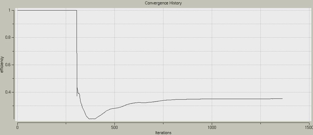
91 Figure 39: Global Residuals for Steady-State Simulations Figure 40: Mass flow rate Convergence for Steady-State Simulations Figure 41: Efficiency Convergence for Steady State Simulations 80