A study of some morphological operators in simplicial complex spaces

Transcription

1 A study of some morphological operators in simplicial complex spaces Fabio Augusto Salve Dias To cite this version: Fabio Augusto Salve Dias. A study of some morphological operators in simplicial complex spaces. Other [cs.oh]. Université Paris-Est, English. <NNT : 2012PEST1104>. <pastel > HAL Id: pastel Submitted on 22 May 2013 HAL is a multi-disciplinary open access archive for the deposit and dissemination of scientific research documents, whether they are published or not. The documents may come from teaching and research institutions in France or abroad, or from public or private research centers. L archive ouverte pluridisciplinaire HAL, est destinée au dépôt et à la diffusion de documents scientifiques de niveau recherche, publiés ou non, émanant des établissements d enseignement et de recherche français ou étrangers, des laboratoires publics ou privés.

2 École Doctorale Mathématiques et Sciences et Technologies de l Information et de la Communication Thèse de doctorat en Informatique Fábio Augusto SALVE DIAS A study of some morphological operators in simplicial complex spaces Une étude de certains opérateurs morphologiques dans les complexes simpliciaux Jury: Thèse dirigée par Laurent NAJMAN Co-encadré par Jean COUSTY Soutenue le 21/09/2012 Laurent NAJMAN, ESIEE Paris, France Jean COUSTY, ESIEE Paris, France Isabelle BLOCH, ENST, France Nicholas PASSAT, Université de Strasbourg, France Dominique JEULIN, CMM - Mines ParisTech, France

3

4 Abstract In this work we study the framework of mathematical morphology on simplicial complex spaces. Simplicial complexes are a versatile and widely used structure to represent multidimensional data, such as meshes, that are tridimensional complexes, or graphs, that can be interpreted as bidimensional complexes. Mathematical morphology is one of the most powerful frameworks for image processing, including the processing of digital structures, and is heavily used for many applications. However, mathematical morphology operators on simplicial complex spaces is not a concept fully developped in the literature. In this work, we review some classical operators from simplicial complexes under the light of mathematical morphology, to show that they are morphology operators. We define some basic lattices and operators acting on these lattices: dilations, erosions, openings, closings and alternating sequential filters, including their extension to weighted simplexes. However, the main contributions of this work are what we called dimensional operators, small, versatile operators that can be used to define new operators on simplicial complexes, while mantaining properties from mathematical morphology. These operators can also be used to express virtually any operator from the literature. We illustrate all the defined operators and compare the alternating sequential filters against filters defined in the literature, where our filters show better results for removal of small, intense, noise from binary images. Keywords: Mathematical morphology, simplicial complexes, granulometries, meshes, alternating sequential filters, image filtering. 2

5 Résumé Dans ce travail, nous étudions le cadre de la morphologie mathématique sur les complexes simpliciaux. Complexes simpliciaux sont une structure versatile et largement utilisée pour représenter des données multidimensionnelles, telles que des maillages, qui sont des complexes tridimensionnels, ou des graphes, qui peuvent être interprétées comme des complexes bidimensionnels. La morphologie mathématique est l un des cadres les plus puissants pour le traitement de l image, y compris le traitement des structures numériques, et est largement utilisé pour de nombreuses applications. Toutefois, les opérateurs de morphologie mathématique sur des espaces complexes simpliciaux n est pas un concept entièrement développé dans la littérature. Dans ce travail, nous passons en revue certains opérateurs classiques des complexes simpliciaux sous la lumière de la morphologie mathématique, de montrer qu ils sont des opérateurs de morphologie. Nous définissons certains treillis de base et les opérateurs agissant sur ces treillis : dilatations, érosions, ouvertures, fermetures et filtres alternés séquentiels, et aussi leur extension à simplexes pondérés. Cependant, les principales contributions de ce travail sont ce que nous appelions les opérateurs dimensionnels, petites et polyvalents opérateurs qui peuvent être utilisés pour définir de nouveaux opérateurs sur les complexes simpliciaux, qui garde les propriétés de la morphologie mathématique. Ces opérateurs peuvent également être utilisés pour exprimer pratiquement n importe quel opérateur dans la littérature. Nous illustrons les opérateurs définis et nous comparons les filtres alternés séquentiels contre filtres définis dans la littérature, où nos filtres présentent de meilleurs résultats pour l enlèvement du petit, intense bruit des images binaires. Mots clés : Morphologie mathématique, complexes simpliciaux, granulométries, maillages, filtres alterné séquentiel, filtrage d image. 3

6 Résumé étendu Les complexes simpliciaux ont été introduites par Poincaré en 1895 [58] pour étudier la topologie des espaces de dimension arbitraire. Ils sont largement utilisés pour représenter des données multidimensionnelles dans de nombreuses applications, telles la modélisation de réseaux [60], la couverture de capteurs mobiles [19], multi-radio optimisation [61], etc. Sous la forme de maillages, ils sont largement utilisés dans de nombreux contextes pour exprimer des données tridimensionnelles, notamment dans l analyse des éléments finis [85, 46] et la géométrie différentielle [20, 26]. Cette polyvalence est la raison pour laquelle nous avons choisi d utiliser les complexes simpliciaux comme espace de travail. La morphologie mathématique a été introduit par Matheron et Serra en 1964, devenant un cadre puissant pour le traitement et l analyse d images [74]. C est aujourd hui un des principaux cadres pour le traitement non-linéaire des images, fournissant des outils pour de nombreuses applications, telles la suppression du bruit [42, 27], la biométrie [59], la segmentation d images [52, 34], l imagerie médicale [69, 1], la recherche par similarité [40], le traitement des documents [56, 17], l amélioration des empreintes digitales [3, 32] etc. Le cadre de la morphologie mathématique a été étendu par Heijmans et Ronse [30] au cadre des treillis complets, permettant l application à des structures numériques plus complexes, tels les graphes [81, 15, 14, 47], les hypergraphes [9, 77] et les complexes simpliciaux [21, 45]. Malgré la polyvalence de l espace considéré et la puissance du cadre, au mieux de notre connaissance, des opérateurs de morphologie mathématique qui agissant sur des complexes simpliciaux, sont encore un concept peu développé dans la littérature. La principale motivation de ce travail est d explorer ce qui peut être fait en combinant un espace polyvalent avec un puissant cadre d opérateurs. Les principales contributions de ce travail prennent la forme de petits opérateurs que nous introduisons, appelés opérateurs dimensionnels, qui ne sont pas issus des opérateurs classiques. Ces opérateurs sont très flexibles et ils offrent une nouvelle façon de représenter d autres opérateurs. Nous 4

7 Table 1 Résumé des travaux pertinents. Espace utilisé Commentaires Vincent [81] Graphes Structure de graphe utilisée comme relation de voisinage. Cousty et. al. [15, 14] Graphes Les valeurs peuvent être propagées aux arêtes. Meyer and Stawiaski [53] Graphes Les valeurs peuvent être propagées aux arêtes. Bloch and Bretto [9] Hypergraphes Définit quelques treillis et des opérateurs morphologiques. Loménie and Stamon [45] Complexes simpliciaux Traite séparément les faces et les arêtes. This work ([21]) Complexes simpliciaux Les valeurs peuvent être associées à toute simplex et tous les simplices sont traités de façon uniforme. montrons qu ils peuvent être utilisées pour exprimer pratiquement n importe quel opérateur présenté dans la littérature. En utilisant ces opérateurs dimensionnels, nous définissons de nouveaux opérateurs morphologiques, que l on compare à certains opérateurs présentés dans la littérature, en particulier pour l enlèvement du bruit. Le tableau 1 résume brièvement les travaux reliés à ce travail, y compris un article contenant des résultats partiels de cette thèse [21]. Dans ce résumé étendu, nous ne rappellerons pas toutes les définitions que nous utiliserons, issues des complexes simpliciaux et de la morphologie mathématique. Les preuves des propriétés et les opérateurs agissant sur les étoilles ont également été omis. Notations importantes. Dans ce travail, le symbole C désigne un n-complexe, non-vide, avec n N. L ensemble des sous-ensembles de C est notée P(C ). Tout sous-ensemble de C qui est aussi un complexe est appelé sous-complexe (de C ). Nous noterons par C l ensemble des sous-complexes de C. Si X est un sous-ensemble de C, on note X le complément de X (en C ) : X = C \X. Le complément d un souscomplexe de C n est généralement pas un sous-complexe. Tout sous- 5

8 ensemble X de C dont le complément X est un sous-complexe est appelé étoile (dans C ). Nous désignons par S l ensemble des étoiles dans C. Si l on considére les complexes simpliciaux, le treillis le plus évident est l ensemble puissance P(C ), fait de tous les sous-ensembles de C, avec la relation d inclusion. Le supremum est donnée par l opérateur d union et le infimum par l intersection. Ce treillis est désigné par P(C ),,, ou simplement P(C ) si aucune ambiguïté est présente. Ce treillis est complémenté, x P(C ), x P(C ) x x = et x x = C. L ensemble C de tous les subcomplexes de C, ordonné par la relation d inclusion, avec comme supremum l opérateur d union et comme infimum l opérateur d intersection, est aussi un treillis. En outre, C,,, est un sous-treillis de P(C ) parce que C est un sous-ensemble de P(C ), fermé par union et intersection, avec le même supremum C et infimum. Le treillis S,,,, contenant toutes les étoiles de C, muni de la relation d inclusion est également un sous-treillis de P(C ). Cependant, les treillis C et S ne sont pas complémentés, le complément d un sous-complexe est une étoile et viceversa. Dans le domaine des complexes simpliciaux, certains opérateurs sont bien connus, tels que la fermeture et l étoile. Nous définissons la fermeture ˆx et l étoile ˇx de x par : x C, ˆx = {y y x, y } (1) x C, ˇx = {y C x y} (2) L opérateur fermeture donne comme résultat l ensemble de tous les simplexes qui sont sous-ensembles du simplex X, et l étoile donne comme résultat l ensemble des simplexes de C qui contiennent le simplex x. Ces opérateurs peuvent être facilement étendus à des ensembles de simplexes. Les opérateurs Cl : P(C ) P(C ) et St : P(C ) P(C ) sont définies par : X P(C ), Cl = {ˆx x X} (3) X P(C ), St = {ˇx x X} (4) Afin d obtenir des granulométries non triviales sur les complexes, nous restreignons le domaine de définition des opérateurs des équations ci-dessus et nous présentons les érosions adjointes. 6

9 Definition 1. Nous définissons les opérateurs : S C, : C S, A : C S and A : S C par : X S, (X) =Cl(X) (5) Y C, (Y ) =St(Y ) (6) X C, A (X) = {Y S (Y ) X} (7) Y S, A (Y ) = {X C (X) Y } (8) En combinant les opérateurs, et leurs adjoints, on peut définir deux opérateurs, une ouverture et une fermeture. Definition 2. Nous définissons : Property 3. Nous avons : 1. Les opérateurs γ h et φ h agissent sur C. 2. Le opérateur γ h est un ouverture. 3. Le opérateur φ h est un fermeture. γ h = A (9) φ h = A (10) Toutefois, les érosions et dilatations impliquées ci-dessus sont idempotentes, donc toute composition de ces opérateurs suivis par l opérateur adjoint conduira à la même ouverture ou fermeture. Par conséquent, ces opérateurs ne sont pas adaptés pour la construction de granulométries non triviales. Examinons maintenant la composition des dilatations et, ainsi que leurs adjoints, afin d obtenir de nouveaux opérateurs agissant sur les complexes. Definition 4. Nous définissons les opérateurs δ et ε par : Property 5. Nous avons : 1. Les opérateurs δ et ε agissent sur C. 2. Le opérateur δ est un dilatation. 3. Le opérateur ε est un erosion. δ = (11) ε = A A (12) 7

10 4. Le pair (ε, δ) est un adjunction. Soit i N et α un opérateur. Nous utilisons la notation α i pour représenter l itération de l opérateur α, c est-à-dire α i = α }.{{.. α}. i fois Definition 6. Soit i N. Nous définissons les opérateurs γ c i et φ c i par : γ c i =δ i ε i (13) φ c i =ε i δ i (14) En contrôlant le paramètre i, nous pouvons contrôler la quantité d éléments qui seront touchés par les opérateurs. Informellement, en augmentant le nombre d itérations, on obtient de plus grands filtres. Property 7. Soit i N. Nous avons : 1. Les opérateurs γ c i et φ c i agissent sur C. 2. Le opérateur γ c i est un ouverture. 3. Le opérateur φ c i est un fermeture. 4. La famille des opérateurs {γλ c, λ N} est un granulometrie. 5. La famille des opérateurs {φ c λ, λ N} est un anti-granulometrie. En composant les opérateurs à partir d une granulométrie et un antigranulométrie, agissant sur le même treillis, nous pouvons définir des filtres alternés séquentiels. Ces filtres peuvent être utilisés pour éliminer progressivement certaines caractéristiques des ensembles considérés, une approche très utile lorsque la taille des éléments est un facteur déterminant. Definition 8. Soit i N. Nous définissons les filtres ASF c i et ASF c i par : X C, ASF c i(x) = (γ c i φ c i) ( γ c i 1φ c i 1)...(γ c 1 φ c 1) (X) (15) X C, ASF c i (X) = (φ c iγ c i ) ( φ c i 1γ c i 1)...(φ c 1 γ c 1) (X) (16) Le paramètre i contrôle combien d éléments du complexe sont touchés par les opérateurs. En contrôlant les itérations du filtre, on peut définir des opérateurs qui éliminent plus de caractéristiques de l ensemble considéré. Property 9. Soit i N. Les opérateurs ASF c i et ASF c i agissent sur C. 8

11 Alternativement, nous pouvons combiner les opérateurs γ c et φ c avec les opérateurs γ h et φ h pour obtenir différentes ouvertures et fermetures. En utilisant cette procédure, nous visons à obtenir des filtres qui affectent moins d éléments du complexe. Dans ce travail, l opérateur mod représente le résidu commun, qui est le reste d une division entière. La notation représente la parte entière. Definition 10. Soit i N et X C. Nous définissont les opérateurs γ ch φ ch i/2 par : γ ch i/2 = φ ch i/2 = { δ i/2 ε i/2 si i mod 2 = 0 δ i/2 γ h ε i/2 autrement. { ε i/2 δ i/2 si i mod 2 = 0 ε i/2 φ h δ i/2 autrement. i/2 et (17) (18) Lorsque le paramètre i de ces opérateurs est pair, les opérateurs γ h et φ h ne sont pas utilisés, et les opérateurs deviennent identiques aux opérateurs γ c et φ c. Ainsi, ces opérateurs sont capables de fonctionner dans une taille intermédiaire, entre deux itérations successives des autres opérateurs. Property 11. Soit i N. Nous avons : 1. Les opérateurs γ ch i/2 2. L opérateur γ ch i/2 3. L opérateur φ ch i/2 et φch i/2 est un ouverture. est un fermeture. agissent sur C. 4. La famille des opérateurs {γλ/2 ch, λ N} est une granulometrie. 5. La famille des opérateurs {φ ch λ/2, λ N} est une anti-granulometrie. Ces familles d opérateurs sont des granulométries et anti-granulométries, et peuvent être considérées pour de nombreuses applications où la taille du filtre est pertinente, par exemple pour composer des filtres alternés séquentiels, comme nous l avons fait précédemment. Definition 12. Soit i N. Nous définissons les opérateurs ASF ch i/2 et ASF ch i/2 par : X C, ASF ch i/2(x) = ( γi/2φ ch ch i/2 X C, ASF ch i/2(x) = ( φ ch i/2γi/2 ch ) ( γ ch ) ( φ ch (i 1)/2 φ ch (i 1)/2 (i 1)/2 γ ch (i 1)/2 9 ) (... γ ch 1/2 φ1/2) ch (X) (19) ) (... φ ch 1/2 γ1/2) ch (X) (20)

12 Property 13. Soit i N. Les opérateurs ASF ch i/2 et ASF ch i/2 agissent sur C. Pour définir les opérateurs dimensionnels, nous commençons par l introduction d une nouvelle notation qui permet récupérer seulement des simplexes d une dimension donnée. Notations importants. Soit X C et i [0, n], nous désignons par X i l ensemble de tous les i-simplexes de X : X i = {x X dim(x) = i}. En particulier, C i est l ensemble de tous les i-simplexes de C. Nous désignons par P(C i ) l ensemble des sous-ensembles de C i. Nous étendons également la notation de complément, si X C i, le complément est pris à l égard de la dimension considérée, X = C i \X. Soit i N tel que i [0, n]. La structure P(C i ),,, est un treillis. Definition 14. Soit i, j N tel que 0 i < j n. Nous définissons les opérateurs δ + i,j et ε+ i,j agissant de P(C i) dans P(C j ) et les opérateurs δ j,i et ε j,i agissant de P(C j ) dans P(C i ) par : X P(C i ), δ + i,j (X) ={x C j y X, y x} (21) X P(C i ), ε + i,j (X) ={x C j y C i, y x = y X} (22) X P(C j ), δ j,i (X) ={x C i y X, x y} (23) X P(C j ), ε j,i (X) ={x C i y C j, x y = y X} (24) En d autres termes, δ + i,j (X) est l ensemble de tous les j-simplexes de C qui comprennent un i-simplexe de X, δ j,i (X) est l ensemble de tous les i- simplexes de C qui sont inclus dans un j-simplex de X, ε + i,j (X) est l ensemble de tous les j-simplexes de C, dont les sous-ensembles de dimension i appartiennent tous à X, et ε j,i (X) est l ensemble de tous les i-simplexes de C qui ne sont pas contenues dans les j-simplexes de X. Property 15. Soit i, j N tels que 0 i < j n. 1. Les paires (ε + i,j, δ j,i ) et (ε j,i, δ+ i,j ) sont des adjunctions. 2. L opérateur δ + i,j est dual de l opérateur ε+ i,j X C i, ε + i,j (X) = C j \ δ + i,j (C i \ X). 3. L opérateur δ j,i est dual de l opérateur ε j,i X C j, ε j,i (X) = C i \ δ j,i (C j \ X). 10

13 Basé sur le comportement attendu des opérateurs ouverture et de fermeture, qui est, la suppression progressive des petits éléments du sous-ensemble considéré, dans notre cas, un complexe contenue dans C, et le complément de la partie, respectivement, nous pouvons définir deux opérateurs simples en utilisant les opérateurs dimensionnelles. Definition 16. Soit d N tel que 0 < d n. Nous définissons les opérateurs γd m et φ m d par : X C, γd m (X) = δ d,i (X d) X i (25) i [0,d 1] i [d,n] X C, φ m d (X) = X i ε + n d,i (X n d) (26) i [0,n d] i [n d+1,n] Property 17. Soit d N tel que 0 < d n. Nous avons : 1. Les opérateurs γ m d et φm d agissent sur C. 2. L opérateur γ m d 3. L opérateur φ m d est une ouverture. est une fermeture. Parce que le paramètre d de ces opérateurs est limité par la dimension de l espace considéré, les tailles possibles des filtres sont également limités. Pour créer des filtres qui peuvent avoir des tailles arbitraires, nous pouvons enrichir les opérateurs γ c et φ c en les composant avec les opérateurs γ m et φ m. Definition 18. Soit i N. Nous définissons les opérateurs γi/(n+1) cm par : et φcm i/(n+1) X C, γ cm i/(n+1)(x) =δ i/(n+1) γ m (i mod (n+1))ε i/(n+1) (X) (27) X C, φ cm i/(n+1)(x) =ε i/(n+1) φ m (i mod (n+1))δ i/(n+1) (X) (28) Property 19. Soit i N. Nous avons : 1. Les opérateurs γ cm i/(n+1) 2. L opérateur γ cm i/(n+1) 3. L opérateur φ cm i/(n+1) et φcm i/(n+1) est une ouverture. est une fermeture. agissent sur C. 4. La famille des opérateurs {γλ/(n+1) cm, λ N} est une granulometrie. 11

14 5. La famille des opérateurs {φ cm λ/(n+1), λ N} est une anti-granulometrie. Definition 20. X C, ASF cm i/(n+1)(x) = ( ) ( γi/(n+1)φ cm cm i/(n+1) γ cm (i 1)/(n+1) φ(i 1)/(n+1)) cm ( γ1/(n+1)φ1/(n+1)) cm cm (X) (29) X C, ASF cm i/(n+1)(x) = ( ) ( φ cm i/(n+1)γi/(n+1) cm φ cm (i 1)/(n+1) γ(i 1)/(n+1)) cm ( φ cm 1/(n+1)γ1/(n+1)) cm (X) (30) Nous pouvons aussi utiliser les opérateurs dimensionnels pour définir de nouveaux opérateurs par composition, conduisant à de nouvelles dilatations, érosions, ouvertures, fermetures et filtres alternés séquentiels. Avant de commencer la composition de ces opérateurs, nous allons examiner les résultats suivants, qui peuvent guider l exploration de nouvelles compositions. Property 21. Soit i, j, k N tels que 0 i < j < k n. 1. X P(C i ), δ + j,k δ+ i,j (X) = δ+ i,k (X) 2. X P(C i ), ε + j,k ε+ i,j (X) = ε+ i,k (X) 3. X P(C k ), δ j,i δ k,j (X) = δ k,i (X) 4. X P(C k ), ε j,i ε k,j (X) = ε k,i (X) En d autres termes, cette propriété indique que toute composition du même opérateur est équivalent à l opérateur agissant de la première dimension à la dimension finale. Property 22. Soit i, j, k N tels que 0 i < j < k n. 1. X P(C i ), δ j,i δ+ i,j (X) = δ k,i δ+ i,k (X) 2. X P(C i ), ε j,i ε+ i,j (X) = ε k,i ε+ i,k (X) 3. X P(C i ), ε j,i δ+ i,j (X) = ε k,i δ+ i,k (X) 4. X P(C i ), δ j,i ε+ i,j (X) = δ k,i ε+ i,k (X) En d autres termes, cette propriété signifie que le résultat des compositions de dilatations et d érosions qui utilisent une dimension supérieure intermédiaire est indépendante de la dimension exacte choisie. Par conséquent, nous pouvons obtenir une seule dilatation de base, une érosion de base, une ouverture et une fermeture à l aide de ces compositions. Toutefois, ce n est pas tout à fait vrai si l on considère une dimension inférieure comme dimension intermédiaire pour les compositions, comme suit : 12

15 Property 23. Soit i, j, k N tels que 0 i < j < k n. 1. X P(C k ), δ + i,k δ k,i (X) δ+ j,k δ k,j (X) 2. X P(C k ), ε + i,k ε k,i (X) ε+ j,k ε k,j (X) 3. X P(C k ), ε + i,k δ k,i (X) = ε+ j,k δ k,j (X) 4. X P(C k ), δ + i,k ε k,i (X) = δ+ j,k ε k,j (X) Jusqu à présent, nous avons présenté les opérateurs dimensionnelles et certaines propriétés pertinentes. En utilisant ces opérateurs, nous avons défini de nouveaux opérateurs et les avons combiné avec les opérateurs classiques. Maintenant, nous présentons de nouvelles adjonctions, fondées uniquement sur les opérateurs dimensionnelles. En utilisant ces adjonctions, nous définissons les ouvertures, fermetures et filtres séquentiels alternés, lorsque c est possible. Definition 24. Nous définissons : { } X C, δ þ (X) = i [0...(n 1)] δ i+1,i δ+ i,i+1 (X { i) δ + n 1,nδn,n 1(X n ) } (31) X C, ε þ (X) =Cl A ({ i [0...(n 1)] ε i+1,i ε+ i,i+1 (X i)}... Property 25. Nous avons :... { ε + n 1,nε n,n 1(X n ) } ) (32) 1. Les opérateurs δ þ, ε þ, δ ß et ε ß agissent sur C. 2. Les paires d opérateurs (ε þ, δ þ ) et (ε ß, δ ß ) sont des adjunctions. Comme nous l avons fait avec les opérateurs des sections précédentes, nous pouvons composer ces opérateurs pour définir de nouveaux opérateurs. Definition 26. Soit i N. Nous définissons : γ þ i φ þ i = ( δ þ) i ( ε þ ) i = ( ε þ) i ( δ þ ) i (33) (34) Property 27. Soit i N. Nous avons : 1. Les opérateurs γ þ i et φ þ i agissent sur C. 13

16 2. Les opérateurs γ þ i sont des ouvertures. 3. Les opérateurs φ þ i sont des fermetures. 4. Le famille d opérateurs {γ þ λ, λ N} est une granulometrie. 5. Le famille d opérateurs {φ þ λ, λ N} est une anti-granulometrie. Étant donné que ces familles agissent sur des sous-complexes et sont des granulométries et des anti-granulométries, nous pouvons les composer pour définir plus de filtres alternées séquentiels. Definition 28. Soit i N. Nous définissons : ) ( X C, ASF þ i (γ (X) = þ i φþ i γ þ (i 1) φþ (i 1) ( ) ( X C, ASF þ i (X) = φ þ i γþ i φ þ (i 1) γþ (i 1) ) (... )... ) γ þ 1 φ þ 1 (X) (35) ( ) φ þ 1 γ þ 1 (X) (36) Property 29. Soit i N. Les opérateurs ASF þ i et ASF þ i, agissent sur C. La figure ci-dessous montre une comparaison entre les meilleurs résultats obtenus par nos opérateurs par rapport aux opérateurs de la littérature, sur le problème de suppression du bruit d une image binaire. Dans ce travail, nous avons exploré certains opérateurs du cadre de la morphologie mathématique agissant sur des complexes simpliciaux. Nous avons commencé par analyser les opérateurs classiques du domaine des complexes simpliciaux dans le cadre des concepts de la morphologie mathématique. En utilisant ces opérateurs, nous avons créé de nouvelles dilatations, érosions, ouvertures, fermetures et filtres alternées séquentiels qui sont en concurrence avec les opérateurs présents dans la littérature. Nous avons ensuite présenté la contribution principale de ce travail, les opérateurs dimensionnels, qui peuvent être utilisés pour définir de nouveaux opérateurs. De nouveaux opérateurs ont été présentés et nous avons démontré que les opérateurs dimensionnels peut être utilisé pour exprimer les opérateurs de la littérature, agissant sur des complexes et des graphes. 14

17 (a) L image originale. ([15]). (b) Version bruitée de l image. ([15]), MSE = 19.56%. (c) ASF classique, 3 itérations. M SE = 13.91%. (d) ASF classique, 9 itérations et 3x résolution. M SE = 2.54%. (e) Graphe ASF 6/2 [15]. MSE = 3.27%. (f) ASF c 3. MSE = 1.91%. Figure 1 Comparaison avec les résultats de la littérature. 15

18 Acknowledgements This work has been funded by Conseil Général de Seine-Saint-Denis and french Ministry of Finances through the FUI6 project Demat- Factory. Once again I am in this situation and everyone that knows me, even just a little, is probably aware that I am positively horrible with names. Completely awful. Embarrasingly so. And it is not limited to people s names, but also mathematical names, like theorems or properties, cars, objects and so on. Pretty much anything with a name attached to it I will promptly and switfly disassociate. But I am abusing the liberty of this section to digress... I would like to thank my family, my advisors, the members of my jury, the students, other professors and everyone else that, directly or indirectly, made this work possible. I came closer than I would care to admit of not getting it done with your help, I cannot bear to imagine where I would have ended up without it.... Burn the land and boil the sea, you can t take the sky from me... 16

19 Publications Directly related to this work: Cousty, J., Najman, L., Dias, F., Serra, J.: Morphological filtering on graphs. Tech. rep., Laboratoire d Informatique Gaspard-Monge - LIGM (2012), Dias, F., Cousty, J., Najman, L.: Some morphological operators on simplicial complex spaces. In: Debled-Rennesson, I., Domenjoud, E., Kerautret, B., Even, P. (eds.) Discrete Geometry for Computer Imagery, Lecture Notes in Computer Science, vol. 6607, pp Springer Berlin / Heidelberg (2011) Additional publications: Silvatti, A.P., Cerveri, P., Telles, T., Dias, F.A.S., Baroni, G., Barros, R.M.: Quantitative underwater 3d motion analysis using submerged video cameras: accuracy analysis and trajectory reconstruction. Computer Methods in Biomechanics and Biomedical Engineering, 1-9 (2012) Silvatti, A.P., Dias, F.A.S., Cerveri, P., Barros, R.M.: Comparison of different camera calibration approaches for underwater applications. Journal of Biomechanics 45(6), (2012) Silvatti, A.P., Telles, T., Dias, F.A.S., Cerveri, P., Barros, R.M.L.: Underwater comparison of wand and 2d plane nonlinear camera calibration methods. In: International Congress of Biomechanics in Sport. (2011) Silvatti, A.P., Telles, T., Rossi, M., Dias, F., Leite, N.J., Barros, R.M.L.: Underwater non-linear camera calibration: an accuracy analysis. In: International Congress of Biomechanics in Sport. (2010) Silvatti, A.P., Rossi, M., Dias, F., Leite, N.J., Barros, R.M.L.: Nonlinear camera calibration for 3d reconstruction using straight line plane object. In: International Conference on Biomechanics in Sport. (2009) 17

20 Contents 1 Introduction and related work 22 2 Basic theoretical concepts Simplicial complexes Mathematical morphology Proposed operators Classical approach: P(C ), C and S Dimensional operators Morphological operators on C using a higher intermediary dimension Morphological operators on C using a lower intermediary dimension Extension to weighted complexes Revisiting the related work Summary of the proposed operators Experimental results Illustration on a tridimensional mesh Illustration on regular images Illustration on a grayscale image Results on a set of regular images Implementational considerations Conclusion

21 List of Figures 1 Comparaison avec les résultats de la littérature Graphical representation of simplexes, complexes and cells Graphical examples of a complex containing a subcomplex and a star Hasse diagram of the lattice of a set Illustration of morphological dilations and erosions Illustration of operators φ h, γ h, Γ h and Φ h Illustration of operators φ c 1, γ1, c Φ c 1 and Γ c Illustration of operators φ ch i/2, γch i/ Illustration of the operators δ + i,j, δ j,i, ε+ i,j and ε j,i Example diagram for the operation Y = γ2 m (X), with n = Illustration of the operators γd m and φm d on complexes Example of the operation Y = δ þ (X), with n = Illustration of morphological dilations and erosions Illustration of operators γ þ i and φ þ i Illustration of operators γ þh i/2, γþm i/(n+1), φþh i/2 and φþm i/(n+1) Example diagram of the threshold decomposition and stacking reconstruction [22] Diagram depicting the relationship between the operators defined Rendering of the mesh considered, the result of a thresholding operation on the curvature values and the results of the operators. The thresholded sets are represented in black Example of the method used to construct a simplicial complex based on a regular image Original test image and its noisy version MSE versus size of the filter for the operators ASF c and ASF c MSE versus size of the filter for the operators ASF ch and ASF ch

22 4.6 MSE versus size of the filter for the operators ASF cm and ASF cm MSE versus size of the filter for the operators ASF þ and ASF þ Illustration of the best results obtained with the operators based on ASF c Illustration of the best results obtained with the operators ASF þ Comparison with some of the literature results Photomicrograph of bone marrow showing abnormal mononuclear megakaryocytes typical of 5q syndrome Zoom of the same section of the image after closings of size Considered set of images Zoom of a section of the same image on all datasets Sixth dataset considered. Average MSE = 26.90% Error versus size of the filter for all sets of noisy images using the operator ASF c Error versus size of the filter for all sets of noisy images using the operator ASF c Error versus size of the filter for all sets of noisy images using the operator ASF ch Error versus size of the filter for all sets of noisy images using the operator ASF ch Error versus size of the filter for all sets of noisy images using the operator ASF cm Error versus size of the filter for all sets of noisy images using the operator ASF cm Error versus size of the filter for all sets of noisy images using the operator ASF þ Error versus size of the filter for all sets of noisy images using the operator ASF þ Error versus size of the filter for all sets of noisy images using the classic ASF operator Error versus size of the filter for all sets of noisy images using the classic ASF operator and triple resolution Error versus size of the filter for all sets of noisy images using the graph ASF [15] Results of the operator ASF c 6 on the sixth dataset. Average MSE = 1.17% Results of the classical ASF with triple resolution and size 7 1 / 3 for the sixth dataset. Average MSE = 1.62%

23 List of Tables 1 Résumé des travaux pertinents Summary of the related works Summary of the dilation operators defined on this work Summary of the erosion operators defined on this work Summary of the opening operators defined on this work Summary of the closing operators defined on this work Summary of the alternating sequential filters acting on C defined on this work Summary of the best results of operators ASF c and ASF c for all datasets Summary of the best results of operators ASF ch and ASF ch for all datasets Summary of the best results of operators ASF cm and ASF cm for all datasets Summary of the best results of operators ASF þ and ASF þ for all datasets Summary of the best results of the classic ASF operator, with normal and triple resolution, and the graph ASF [15] for all datasets

24 Chapter 1 Introduction and related work Simplicial complexes were first introduced by Poincaré in 1895 [58] to study the topology of spaces of arbitrary dimension, and are basic tools for algebraic topology [48], homotopy by collapse [84], image analysis [37, 8, 12], discrete surfaces [23, 24, 16]. They are widely used to represent multidimensional data in many applications, such as modelling networks [60], mobile sensors coverage [19], multi-radio broadcasting optimization [61] and even in pattern recognition, to find symmetries in musics, where each music is represented as a complex [62]. In [44], simplicial complexes are used to capture the topological information about the visual coverage of a camera network, used for object tracking. A similar structure, the cubical complex, often called cellular complex, is also considered as space for image processing [38, 39], including a version of the Jordan theorem [35]. They can also be considered to represent tridimensional data [57]. We will not explore cubical complexes in this work, but, since many properties and definitions also hold for cubical complexes, we will mention, briefly, what does not hold for cubical complexes. In the form of meshes they are widely used in many contexts to express tridimensional data, notably for finite elements analysis [85, 46] and digital exterior calculus [20, 26]. Some graphs can be represented as a form of simplicial complexes, and we can build simplicial complex based on regular, matricial, images, as we will demonstrate further in this work. This versatility was the reason we chose to use simplicial complexes as the operating space. However, we will put aside, momentarily, the practical applications mentioned and focus on developing operators that act on simplicial complexes. Usually, such operators act on the structure of the complex. For instance, it is fairly common to change the complexity of the mesh structure [18, 11]. Even when additional data is associated with the elements of the complex, 22

25 they are mostly used to guide the change of the structure, the values themselves are not changed. We pursuit a different option, in this work, our objective is to filter values associated to the elements of the complex, without changing its structure, using the framework of mathematical morphology. Mathematical morphology was introduced by Matheron and Serra in 1964, becoming a powerful framework for image analysis and processing [74]. It has become one of the most important frameworks for non-linear image processing, with applications wherever an image can be found, providing tools for great many applications, such as noise removing [42, 27], biometrics [59], image segmentation [52, 34], medical imaging [69, 1], pattern matching, similarity search [40], document processing [56, 17], fingerprint enhancement [3, 32] and so on. The framework of mathematical morphology was later extended by Heijmans and Ronse [30] using complete lattices, allowing the application of the framework on more complex digital structures, such as graphs [81, 15, 14, 47], hypergraphs [9, 77] and simplicial complexes [21, 45]. The various operators [74, 70, 75, 55] created by mathematical morphology stem from the two sources of an adjunction and of a connection. The first one leads to theory of openings and closings by adjunction [29, 64, 28], and then, to morphological filters. The second source, a general study of which can be found in [73], introduces and studies connections [71, 66], regional minima, flat zones processing [82, 68, 10, 54], levellings [49, 50, 72], watersheds [83, 7, 13], homotopic thinning [36, 6] and so on. The two sources are not incompatible, and one can combine their axioms (e.g. a connected opening). In practice the first line expresses mainly filtering, whereas the second one focuses on segmentation. The present thesis is exclusively devoted to the building up of adjunctions, and to its consequences in terms of filtering. Despite the versatility of the considered space and the power of the framework, to the best of our knowledge, operators from mathematical morphology, acting on simplicial complexes, are still an undeveloped concept in the literature. The main motivation of this work is to explore what can be achieved by combining a versatile space with a powerful framework of operators. Simplicial complexes and mathematical morphology are not incompatible, it is well known, and we also demonstrate, that some classical operators from simplicial complexes are in fact morphological operators. However, the way we interpret these operators is new, and we use them as starting point to develop new operators. We define dilations, erosions, openings, closings and alternating sequential filters, based on these well known operators from simplicial complexes. We chose to develop these operators because they are some of the most basic operators one can consider when using mathematical morphology, that is, they can be used as tools to build other applications or 23

26 operators. However, the main contributions of this work are the small operators we introduce, called dimensional operators, that are not derived from the classic operators. These operators provide a new and very flexible way to represent operators, and we show that they can be used to express virtually any operator presented in the literature. Using the dimensional operators, we define new morphological operators, that we compare against some operators presented in the literature, considering noise removal. The idea to use a digital structure to image processing is not new. In [81], Vincent uses the lattice approach to mathematical morphology to define morphological operators on neighborhood graphs [67], where the graph structure is used to define neighborhood relationships between unorganized data, expressed as vertices. The same idea is further explored by Barrera et al. [5]. Some morphological operators can also be obtained by using the Image Foresting transform [25], that also explores the idea of using a graph to express neighborhood relationship between data points. By allowing the vertices values to be propagated to the edges, therefore using the graph structure to express more than just neighborhood relation, Cousty et al. [15] obtained different morphological operators, including openings, closings and alternating sequential filters. Those operators are capable of dealing with smaller noise, effectivelly acting in a smaller size than the classical operators. Similar operators were also used by Meyer and Stawiaski [53] and by Meyer and Angulo [51] to obtain a new approach to image segmentation and levellings, respectively. In [78], Ta et al. use partial differential equations [4] to define morphological operators on weighted graphs, extending the PDE-based approach to the processing of high dimensional data. Recently, Block and Bretto [9] introduced mathematical morphology on hypergraphs, defining lattices and operators on this domain. Their lattices and operators are similar to the ones presented in this work, respected the differences between hypergraphs and complexes. This work is focused on mathematical morphology on simplicial complexes, specifically to process values associated to elements of the complex in an unified manner, without altering the structure itself. In [45], Loménie and Stamon explore mathematical morphology operators on mesh spaces provenient from point spaces. However, the complex only provides structural information, while the information itself is associated only to triangles or edges of the mesh. Table 1.1 briefly summarizes the related works that are more relevant for this work, including an article containing partial results of this work [21]. In chapter 2 we remind the basic concepts and definitions of simplicial 24

27 Table 1.1: Summary of the related works. Considered Comments space Vincent [81] Graphs Graph structure used as neighborhood relation. Cousty et. al. [15, 14] Graphs Values can be propagated to edges. Meyer and Stawiaski [53] Graphs Values can be propagated to edges. Bloch and Bretto [9] Hypergraphs Defines several lattices and Loménie and Stamon [45] This work ([21]) Simplicial complexes Simplicial complexes morphological operators. Processes separately faces and edges. Values can be associated with any simplex and all simplices are treated uniformly. complexes and mathematical morphology used in this work, leading to operators from mathematical morphology acting on simplicial complexes, presented on chapter 3. In that chapter we present operators based on the classical operators from simplicial complexes and new basic operators, called dimensional operators, that are the main contribution of this work. Using these dimensional operators, we define new operators acting on simplicial complexes and we can also express the operators presented in the literature. Since we extend these operators to weighted complexes, using threshold decomposition and stacking, all the operators presented can be applied on weighted complexes. Some illustrations and experimental results are presented in chapter 4, using values associated with elements of a tridimensional mesh, regular binary and grayscale images. We also analyse the noise removal capabilities of our filters on sets of regular images with varying amounts of small noise. 25

28 Chapter 2 Basic theoretical concepts The objective of this work is to explore mathematical morphology on simplicial complex spaces. To this end, we start by reminding useful definitions about simplicial complexes, in section 2.1, and mathematical morphology, in section Simplicial complexes One of the most known forms of complex [33] is the concept of mesh, often used to express tridimensional data on various domains, such as computer aided design, animation and computer graphics in general. However, in this work we prefer to approach complexes by the combinatorial definition of an abstract complex. The basic element of a complex is a simplex. In this work, a simplex is a finite, nonempty set. The dimension of a simplex x, denoted by dim(x), is the number of its elements minus one. A simplex of dimension n is also called an n-simplex. Figure 2.1(a) (resp. 2.1(b), and 2.1(c)) graphically represents a simplex x = {a} (resp. y = {a, b} and z = {a, b, c}) of dimension 0 (resp. 1, 2). Figure 2.1(d) shows a set of simplices composed of one 2-simplex ({a, b, c}), three 1-simplices ({a, b}, {b, c} and {a, c}) and three 0-simplices ({a}, {b} and {c}). We call simplicial complex, or simply complex, any set X of simplices such that, for any x X, any non-empty subset of x also belongs to X. The dimension of a complex is equal to the greatest dimension of its simplices. In the following, a complex of dimension n is also called an n-complex. For instance, figure 2.1(d) represents an elementary 2-complex. Figure 2.2(a) shows another 2-complex. 26

29 (a) A 0-simplex. (b) A 1-simplex. (c) A 2-simplex. (d) A 2-cell Figure 2.1: Graphical representation of simplexes, complexes and cells. Important notations. In this work, the symbol C denotes a nonempty n-complex, with n N. The set of all subsets of C is denoted by P(C ). Any subset of C that is also a complex is called a subcomplex (of C ). We denote by C the set of all subcomplexes of C. A subcomplex X of C is called a cell of C if there exists a simplex x in X such that X is the set of all subsets of x. As an example, the 2-complex depicted on figure 2.1(d) is also a 2-cell. The subset {{a}, {b}, {a, b}} of this complex is a 1-subcomplex and also a 1-cell. The set of gray simplices depicted in figure 2.2(a) is a 2-subcomplex. Any subcomplex X C is generated, using the union operator, by the family G of all cells of C that are included in X: X = {Y G}. Conversely, any family G of cells generates, using the union operator, an element of C. In this sense, the cells can be seen as the elementary building blocks of the complexes. If X is a subset of C, we denote by X the complement of X (in C ): X = C \X. The complement of a subcomplex of C is usually not a subcomplex. Any subset X of C whose complement X is a subcomplex is called a star (in C ). For instance, the gray set of simplices of figure 2.2(a), is a subcomplex, but its complement, the set of black simplices, is, by definition, a star. Similarly, the gray set of figure 2.2(b) is a star, and the black set is a subcomplex. We denote by S the set of all stars in C. The intersection C S is non-empty since it always contains at least and C. In this section we presented some basic definitions and properties regarding simplicial complexes. We will consider simplicial complexes as operating space for the operators defined on the next chapters. 27

30 (a) A complex containing a subcomplex. (b) A complex containing a star. Figure 2.2: Graphical examples of a complex containing a subcomplex and a star. 2.2 Mathematical morphology Our goal is to investigate morphological operators acting on simplicial complexes. The previous section presented a brief reminder of the involved concepts from that domain. In this section we remind the basic concepts of mathematical morphology. In this work, we approach mathematical morphology through the framework of lattices [63]. We start with the concept of partially ordered set (poset). It is composed by a set and a binary relation. The binary relation is defined only between certain pairs of elements of the set, representing precedence, and must be reflexive, antisymmetric and transitive. A lattice is a poset with a least upper bound, called supremum, and a greatest lower bound, called infimum. For instance, consider the set P(S) = {{a, b, c}, {a, b}, {a, c}, {b, c}, {a}, {b}, {c}}, the power set of the set S = {a, b, c}. This set, ordered by the inclusion relation, is a lattice. The supremum of two elements of this lattice is given by the union operator and the infimum by the intersection operator. This lattice can be denoted by P(S),,,. A lattice is complemented if the complement of any given element of the lattice also belongs to the lattice. A graphical representation of this lattice, known as Hasse diagram, is shown on figure 2.3. In such diagram, two sets x 1 and x 2 are linked if x 1 x 2 and there is no set x 3 such that x 1 x 3 x 2. In mathematical morphology (see, e.g., [65]), any operator that associates elements of a lattice L 1 to elements of a lattice L 2 is called a dilation if it commutes with the supremum. Similarly, an operator that commutes with the infimum is called an erosion. Let L 1 and L 2 be two lattices whose order relations and suprema are denoted by 1, 2, 1, and 2. Two operators α : L 2 L 1 and β : L 1 L 2 28

31 Figure 2.3: Hasse diagram of the lattice of a set. form an adjunction (β, α) if α(a) 1 b a 2 β(b) for every element a in L 2 and b in L 1. It is well known (see, e.g., [65]) that, given two operators α and β, if the pair (β, α) is an adjunction, then β is an erosion and α is a dilation. Furthermore, if α is a dilation, the following relation characterizes its adjoint erosion β [65]: a L 1, β(a) = 2 {b L 2 α(b) 1 a} (2.1) We will, in certain cases, express the adjoint operator of an operator α as α A, to explicit the relationship between them. In mathematical morphology, an operator α, acting on a lattice L, that is increasing ( A, B L, A B = α(a) α(b)) and idempotent ( A L, α(a) = α(α(a))) is a filter. If a filter is anti-extensive ( A L, α(a) A) it is called an opening. Similarly, an extensive filter ( A L, A α(a)) is called a closing. One easy way of obtaining openings and closings is by combining dilations and erosions [65]. Let α : L L be a dilation. We can obtain a closing ζ and an opening ψ acting on L by: ζ = α A α (2.2) ψ = αα A (2.3) A family of openings Ψ = {ψ λ, λ N} acting on L, is a granulometry if, given two positive integers i and j, we have i j = ψ i (a) ψ j (a), for any a L [65]. Similarly, a family of closings Z = {ζ λ, λ 0}, is a anti-granulometry if, given two positive integers i and j, we have i j = ψ i (a) ψ j (a), for any a L. A family of filters {α λ, λ N} is a family of alternating sequential filters if, given two positive integers i and j, we have i > j = α i α j = α i, for any a L [65]. 29

32 Let Ψ = {ψ λ, λ N} be a granulometry and Z = {ζ λ, λ N} be an antigranulometry. We can construct two alternating sequential filters (ASF) by composing operators from both families [65]. Let i N: X L, ν i (X) = (ψ i ζ i )(ψ i 1 ζ i 1 )...(ψ 1 ζ 1 ) (X) (2.4) X L, ν i(x) = (ζ i ψ i )(ζ i 1 ψ i 1 )...(ζ 1 ψ 1 ) (X) (2.5) In this section we presented a brief reminder of the concepts of mathematical morphology that will be explored in the next chapters, considered in the context of simplicial complexes. 30

33 Chapter 3 Proposed operators In this chapter we will present new mathematical morphology operators acting on lattices of simplicial complexes. This is the main contribution of this work, more specifically the dimensional operators presented on section Classical approach: P(C ), C and S. Considering simplicial complexes, the most obvious lattice we can define is the power set P(C ), made of all subsets of C, together with the inclusion relation. The supremum operator is given by the union and the infimum operator by the intersection. This lattice is denoted by P(C ),,,, or simply P(C ) if no ambiguity is present. This lattice is complemented, that is, x P(C ), x P(C ) x x = and x x = C. The set C of all subcomplexes of C, ordered by the inclusion relation, along with the union as supremum operator and the intersection as infimum operator, is also a lattice. Further, C,,, is a sublattice of P(C ) since C is a subset of P(C ), closed under union and intersection, with the same supremum C and infimum. Similarly, the lattice S,,,, containing the S of all stars of C, equipped with the inclusion relation is also a sublattice of P(C ). However, the lattices C and S are not complemented, since the complement of a subcomplex is a star and vice versa. In the domain of simplicial complexes, some operators are well known, such as the closure and star [33]. We define the closure ˆx and the star ˇx of x as: x C, ˆx = {y y x, y } (3.1) x C, ˇx = {y C x y} (3.2) 31

34 (a) X (b) Y (c) Z (d) V (e) W Figure 3.1: Illustration of morphological dilations and erosions. In other words, the closure operator gives as result the set of all simplices that are subsets of the simplex x, and the star gives as result the set of all simplices of C that contain the simplex x. These operators can be easily extended to sets of simplices. The operators Cl : P(C ) P(C ) and St : P(C ) P(C ) are defined by: X P(C ), Cl(X) = {ˆx x X} (3.3) X P(C ), St(X) = {ˇx x X} (3.4) Both operators commute with the union operator, that is the supremum of the lattice P(C ). Therefore, the operators Cl and St are dilations, acting on P(C ). We can use equation 2.1 to find the adjunct erosions Cl A : P(C ) P(C ) and St A : P(C ) P(C ), as follows: X P(C ), Cl A (X) = {Y P(C ) Cl(Y ) X} (3.5) X P(C ), St A (X) = {Y P(C ) St(Y ) X} (3.6) The four operators presented above are illustrated in the figure 3.1, where the subsets X, Y, Z, V, and W, made of gray simplices in figures 3.1(a), 3.1(b), 3.1(c), 3.1(d), and 3.1(e), satisfy the following relations Y = St(X), Z = St A (X), V = Cl(Y ), W = Cl A (Z). The result of operator St is always a star and the star depicted on figure 3.1(b) is the smallest star that contains X. Similarly, the star depicted on figure 3.1(c) is the greatest star contained in X. The subcomplex depicted in figure 3.1(d) is the smallest complex V that contains Y. The subcomplex depicted in figure 3.1(e) is the greatest subcomplex contained in Z. 32

35 Since the operators Cl and St are dilations, they constitute a straightforward choice to investigate morphology on complexes. However, these dilations are idempotent. The adjunct erosions Cl A and St A are also idempotent. Thus, they lead to trivial granulometries. In order to obtain nontrivial granulometries, one could consider the following compositions: Dil =ClSt (3.7) Er =St A Cl A (3.8) Indeed, the operator Dil : P(C ) P(C ) is a dilation, since it is a composition of dilations [31]. This operator is not idempotent, and its results are always complexes. By the theorem of composition of adjunctions (see [65], p. 59), the erosion Er : P(C ) P(C ) is the adjunct operator of Dil. However, the pair (Er, Dil) does not lead to granulometries acting on complexes, since the result of Er is always a star. In order to obtain nontrivial granulometries on complexes, let us restrict the operators of equations 3.3 and 3.4. Definition 30. We define the operators : S C and : C S by: X S, (X) =Cl(X) (3.9) Y C, (Y ) =St(Y ) (3.10) The only difference between and Cl is the domain of activity of the each operator. A similar remark holds true for and St. The operators and are also obviously two dilations. Then, using again the equation 2.1, the adjoint erosions A and A are given by: Property 31. X C, A (X) = {Y S (Y ) X} (3.11) Y S, A (Y ) = {X C (X) Y } (3.12) The star A (X) is the interior of the complex X and that the complex A (Y ) is the core of the star Y. Therefore, the following property links the adjoint of, St,, and Cl in a surprising way. 33

36 Property 32. The two following propositions hold true: X C, A (X) =St A (X) (3.13) Y S, A (Y ) =Cl A (Y ) (3.14) It is known in topology that the closure and interior operators are dual with respect to the complement. Thus, we deduce the following result. Property 33. The operators and A (resp. and A ) are dual with respect to the complement in P(C ): we have A (X) = ( X ), for any X C (resp. A (Y ) = ( Y ), for any Y S) By using equations 3.11 and 3.12 directly, computing A (X) (resp. A (X)) requires an exponential time since the family of all stars (complexes) must be considered. On the other hand, as the operators Cl and St are locally defined, (X) and (X) can be computed in linear-time. Hence, due to Property 33, A (X) and A (X) can also be computed in linear-time. We can also provide an alternative characterization for the operators from definition 30 and the classical closure and star operators. Property 34. X C (X) ={x C y X, y x} (3.15) Y S, (Y ) ={x C y X, x y} (3.16) Z C, St(Z) ={x C y Z, y x} (3.17) Z C, Cl(Z) ={x C y Z, x y} (3.18) By combining the operators and and their adjoints we can define two pairs of openings and closings. 34

37 Definition 35. We define: γ h = A (3.19) φ h = A (3.20) Γ h = A (3.21) Φ h = A (3.22) The operators φ h, γ h, Φ h and Γ h are illustrated on figure 3.2, with the considered sets in gray. We consider the results for two subcomplexes, Y and Z, and two stars, W and V. As expected, the closing operators added elements to the considered set. For the subcomplex, triangles and edges were included, and edges and points were included for the star. Similarly, the opening operators removed small elements of the set. These images also illustrate the duality w.r.t. the complement between the operators. Property 36. We have: 1. The operators γ h and φ h act on C. 2. The operators Γ h and Φ h act on S. 3. The operators γ h and Γ h are openings. 4. The operators φ h and Φ h are closings. 5. The operators γ h and Φ h are dual of each other, with respect to the complement. 6. The operators φ h and Γ h are dual of each other, with respect to the complement. Proof. 1. Straightforward from the domains of the operators and A for the operator γ h, and from the domains of the operators and A for the operator φ h. 2. Identical to the previous property, considering the change in the order of the operators. 3. Any erosion followed by the adjoint dilation is an opening [65]. 35

38 (a) Y (b) φ h (Y ) (c) Z (d) γ h (Z) (e) W (f) Γ h (W ) (g) V (h) Φ h (V ) Figure 3.2: Illustration of operators φ h, γ h, Γ h and Φ h. 4. Any dilation followed by the adjoint erosion is a closing [65]. 5. Trivial from property 33 and the definition of the operators. 6. Trivial from property 33 and the definition of the operators. In other words, the presented operators act on the desired spaces, C for γ h and φ h, S for Γ h and Φ h, and consist of openings and closings, as expected, and can be use to remove small objects from the considered set or its background. The duality property between the operators can, for instance, ease the implementation of the operators. However, since the erosions and dilations involved are idempotent, any composition of these operators followed by the adjoint operator will lead to the same opening or closing. Therefore these operators are not suitable for constructing nontrivial granulometries. Let us now compose the dilations and, as well as their adjoints, to obtain new operators acting on complexes and stars. 36

39 Definition 37. We define the operators δ, ε, and E by: δ = (3.23) ε = A A (3.24) = (3.25) E = A A (3.26) Figures 3.1(d) and 3.1(e) represent, in gray, the complexes V = δ(x) and W = ε(x), where X is the complex represented in gray in figure 3.1(a). Property 38. Considering the operators from definition 37, we have: 1. The operators δ and ε act on C. 2. The operators and E act on S. 3. The operators δ and are dilations. 4. The operators ε and E are erosions. 5. The pairs (ε, δ) and (E, ) are adjunctions. Proof. 1. Straightforward from the domain of the operators and A. 2. Straightforward from the domain of the operators and A. 3. Operators and are dilations. Compositions of dilations are dilations [65]. 4. Operators A and A are erosions. Compositions of erosions are erosions [65]. 5. Direct application of the theorem of compositions of adjunctions (see, e.g. [65], p. 59). The adjunctions from definition 37 are not idempotent and act on the desired spaces, so they are suitable for building granulometries and antigranulometries. Since the involved lattices are not complemented, these adjunctions are not dual, with respect to the complement. 37

40 Let i N and α an operator. We use the notation α i to represent the iteration of the operator α, that is, α i = α }.{{.. α}. i times Definition 39. Let i N. We define the operators γ c i, φ c i, Γ c i and Φ c i by: γi c =δ i ε i (3.27) φ c i =ε i δ i (3.28) Γ c i = i E i (3.29) Φ c i =E i i (3.30) By controlling the parameter i, we can control the amount of elements that will be affected by the operators. Informally speaking, by increasing the number of iterations, we obtain greater filters. Property 40. Let i N. We have: 1. The operators γ c i and φ c i act on C. 2. The operators Γ c i and Φ c i act on S. 3. The operators γ c i and Γ c i are openings. 4. The operators φ c i and Φ c i are closings. 5. The families of operators {γλ c, λ N} and {Γc λ, λ N} are granulometries. 6. The families of operators {φ c λ, λ N} and {Φc λ, λ N} are antigranulometries. Proof. 1. Trivial from property Trivial from property Compositions of erosions followed by the adjoint dilations are openings [65]. 38

41 (a) Y (b) φ c 1(Y ) (c) Z (d) γ c 1(Z) (e) W (f) Φ c 1(W ) (g) V (h) Γ c 1(V ) Figure 3.3: Illustration of operators φ c 1, γ c 1, Φ c 1 and Γ c Compositions of dilations followed by the adjoint erosions are closings [65]. 5. Since all elements of the families are openings, we need to prove that, for any two non-negative integers λ and µ, we have λ µ = γ c µ γ c λ (resp. λ µ = Γ c µ Γ c λ ). From the definition 39, we have: γc µ = δ µ λ γ c λ εµ λ (resp. Γ c µ = µ λ Γ c λ E µ λ ). Using the Lemma 2.7, equation 2.6, from [31], we easily conclude that γ c µ γ c λ (resp. Γc µ Γ c λ ). 6. Identical to the previous proof, but using equation 2.7 of Lemma 2.7 presented in [31]. In other words, the operators φ c, Φ c, γ c and Γ c are increasing and idempotent, whereas φ c and Φ c are extensive and γ c and Γ c are anti-extensive. Furthermore, since δ, ε, and E are not idempotent, the operators obtained by iterating these operators lead to nontrivial granulometries. The operators φ c, γ c, Φ c and Γ c are illustrated on figure 3.3. We considered two different subcomplexes, Y and Z, and two different stars, W and V. As we expected, the openings removed elements of the sets, whereas the closing included elements. However, these operators affected more elements than the operators illustrated on figure 3.2. Informally speaking, we can consider the operators from definition 35 smaller than the operators from definition 39. By composing the operators from a granulometry and an anti-granulometry, acting on the same lattice, we can define alternating sequential filters, follow- 39

42 ing equations 2.4 and 2.5. These filters can be used to progressively remove features of the considered sets, a very useful approach when the size of the features is a determinant factor. Definition 41. Let i N. We define the alternating sequential filters ASF c i, ASF c i, ASF Sc i and ASF Sc i by: X C, ASF c i(x) = (γ c i φ c i) ( γ c i 1φ c i 1)...(γ c 1 φ c 1) (X) (3.31) X C, ASF c i (X) = (φ c iγ c i ) ( φ c i 1γ c i 1)...(φ c 1 γ c 1) (X) (3.32) Y S, ASF Sc i (Y ) = (Γ c iφ c i) ( Γ c i 1Φ c i 1)...(Γ c 1 Φ c 1) (Y ) (3.33) Y S, ASF Sc i (Y ) = (Φ c iγ c i) ( Φ c i 1Γ c i 1)...(Φ c 1 Γ c 1) (Y ) (3.34) Similarly to the openings and closing defined previously, the parameter i controls how many elements of the complex are affected by the operators. By controlling the iterations of the filter, we can define greater filters, that is, filters that remove greater features of the considered set. Property 42. Let i N. We have: 1. The operators ASF c i and ASF c i act on C. 2. The operators ASF Sc i Proof. Trivial from property 40. and ASF Sc i act on S. Alternatively, we can combine the operators from definition 39 with the operators from definition 35, to obtain different openings and closings. By using this procedure, we aim to obtain filters that affect less elements of the complex, when compared to the filters from definition 39. Informally speaking, we want to obtain filters smaller than the operators from definition 39. In this work, the operator mod represents the common residue, that is, the remainder of an integer division. The notation represents the floor operator. Definition 43. Let i N and X C. We define the operators γ ch φ ch i/2, Γch i/2 and Φch i/2 by: i/2 and 40

43 γ ch i/2 = φ ch i/2 = Γ ch i/2 = Φ ch i/2 = { δ i/2 ε i/2 if i mod 2 = 0 δ i/2 γ h ε i/2 otherwise. { ε i/2 δ i/2 if i mod 2 = 0 ε i/2 φ h δ i/2 otherwise. { i/2 E i/2 if i mod 2 = 0 i/2 Γ h E i/2 otherwise. { E i/2 i/2 if i mod 2 = 0 E i/2 Φ h i/2 otherwise. (3.35) (3.36) (3.37) (3.38) When the parameter i of these operators is even, the operators γ h, φ h, Γ h and Φ h are not used, and the operators become identical to the operators from definition 39. Thus, these operators are very similar to the operators from definition 39, but they are capable of operating in an intermediary size, between two consecutive iterations of the operators from definition 39. Property 44. Let i N. We have: 1. The operators γ ch i/2 2. The operators Γ ch i/2 3. The operators γ ch i/2 4. The operators φ ch i/2 and φch i/2 and Φch i/2 and Γch i/2 and Φch i/2 act on C. act on S. are openings. are closings. 5. The families of operators {γλ/2 ch, λ N} and {Γch granulometries. 6. The families of operators {φ ch λ/2, λ N} and {Φch anti-granulometries. λ/2 λ/2, λ N} are, λ N} are Proof. 1. Trivial from properties 38 and Trivial from properties 38 and

44 (a) Y (b) φ ch 1/2 (Y ) (c) φch 2/2 (Y ) (d) φch 3/2 (Y ) (e) Z (f) γ1/2 ch (Z) (g) γch 2/2 (Z) (h) γch 3/2 (Z) Figure 3.4: Illustration of operators φ ch i/2, γch i/2. 3. Trivial from Preposition 5.2 of [31]. 4. Trivial from Table II of [31]. 5. Identical to the proof of property 40.5, with a special case when i = 1, that is, we still have to prove that γ2/2 ch γch 1/2. Following the definitions, this equation becomes A A A, that is equivalent to Γ h A A, which is true, since Γ h is an opening. A similar procedure can be done for the family {Γ ch λ/2, λ N}. 6. Identical to the proof of property 40.6, considering the special case when i = 1, following the same procedure as we used in the previous item. Figure 3.4 illustrates the operators γ ch i/2 and φch i/2 on two subcomplexes. As expected, by increasing the parameter i, we control how many elements of the complex are affected by the operators. When i = 2, the results are identical to the results of the operators from definition 39, illustrated on figure 3.3. The operators act on the desired spaces, and are closings and openings. The insertion of the operators γ h, φ h, Γ h and Φ h did not interfered with the basic properties of the operators from definition 39. Additionally, these families of operators are also granulometries and anti-granulometries, and can be considered for many applications where the size of the filter is relevant, for instance to compose alternating sequential filters, as we did previously. 42

45 Definition 45. Let i N. We define the alternating sequential filters ASF ch i/2, ASF ch i/2, ASF Sch i/2 and ASFSch i/2 by: X C, ASF ch i/2(x) = ( ) ( ) ( γi/2φ ch ch i/2 γ ch (i 1)/2 φ ch (i 1)/2... γ ch 1/2 φ1/2) ch (X) X C, ASF ch i/2(x) = ( ) ( ) ( φ ch i/2γi/2 ch φ ch (i 1)/2 γ(i 1)/2 ch... φ ch 1/2 γ1/2) ch (X) (3.39) (3.40) Y S, ASF Sch i/2 (Y ) = ( ) ( ) ( Γ ch i/2φ ch i/2 Γ ch (i 1)/2 Φ ch (i 1)/2... Γ ch 1/2 Φ1/2) ch (Y ) (3.41) Y S, ASF Sch i/2 (Y ) = ( ) ( ) ( Φ ch i/2γ ch i/2 Φ ch (i 1)/2 Γ ch (i 1)/2... Φ ch 1/2 Γ1/2) ch (Y ) (3.42) Property 46. Let i N. We have: 1. The alternating sequential filters ASF ch i/2 and ASF ch i/2 act on C. 2. The alternating sequential filters ASF Sch i/2 Proof. Trivial from property 44. and ASFSch i/2 act on S. If we considered only the iterations with an even i, the operators from definition 45 would be identical to the operators from definition 41, because the openings and closings involved would be identical. The additional iterations, using a smaller operator, allows these filters to deal with smaller components of the complex in a consistent way, but also increases their computational cost. 3.2 Dimensional operators In this section we introduce four new basic operators that act on simplices of given dimensions. These operators are the main contribution of this work and can be composed into new operators which behaviour can be finely controlled. We start by introducing a new notation that allows only simplices of a given dimension to be retrieved. Let X C and let i [0, n], we denote by X i the set of all i-simplices of X: X i = {x X dim(x) = i}. In particular, C i is the set of all i-simplices of C. We denote by P(C i ) the set 43

46 of all subsets of C i. We also extend the notation of complement, if X C i, the complement is taken with respect to the considered dimension, that is, X = C i \X. Let i N such that i [0, n]. The structure P(C i ),,, is a lattice. Definition 47. Let i, j N such that 0 i < j n. We define the operators δ + i,j and ε+ i,j acting from P(C i) into P(C j ) and the operators δ j,i and ε j,i acting from P(C j) into P(C i ) by: X P(C i ), δ + i,j (X) ={x C j y X, y x} (3.43) X P(C i ), ε + i,j (X) ={x C j y C i, y x = y X} (3.44) X P(C j ), δ j,i (X) ={x C i y X, x y} (3.45) X P(C j ), ε j,i (X) ={x C i y C j, x y = y X} (3.46) In other words, δ + i,j (X) is the set of all j-simplices of C that include an i-simplex of X, δ j,i (X) is the set of all i-simplices of C that are included in a j-simplex of X, ε + i,j (X) is the set of all j-simplices of C whose subsets of dimension i all belong to X, and ε j,i (X) is the set of all i-simplices of C that are not contained in any j-simplex of X. The dimensional operators from definition 47 are illustrated on figure 3.5, considering a simple 2-complex as the operating space C. The first, third and fifth columns represent the input sets considered for each example. The first row illustrates the operator δ + i,j, for all possible combinations of input and output dimension on this complex. This operator returns all simplices of the output dimension that contain a simplex of the argument set. The second row illustrates the operator δ j,i, that, as expected, returns all simplices of the output dimension that are contained in a simplex of the argument. The third row illustrates the operator ε + i,j, that returns all simplices of the output dimension such that all its components of the input dimension are contained in the argument. For instance, consider the figures 3.5(m) and 3.5(n). The result is the only edge such that all its contained points are also contained in the input set X m. The fourth row illustrates the operator ε j,i, that returns a set of simplices of the output dimension such that, for every simplex, all simplices of the input dimension that contain that simplex belong to the argument. For instance, consider the figures 3.5(w) and 3.5(x). For each edge of the result, all the triangles that contain that edge belong to the 44

47 (a) X a (b) δ + 0,1 (X a) (c) X c (d) δ + 0,2 (X c) (e) X e (f) δ + 1,2 (X e) (g) X g (h) δ 1,0 (X g) (i) X i (j) δ 2,0 (X i) (k) X k (l) δ 2,1 (X k) (m) X m (n) ε + 0,1 (X m) (o) X o (p) ε + 0,2 (X o) (q) X q (r) ε + 1,2 (X q) (s) X s (t) ε 1,0 (X s) (u) X u (v) ε 2,0 (X u) (w) X w (x) ε 2,1 (X w) Figure 3.5: Illustration of the operators δ + i,j, δ j,i, ε+ i,j and ε j,i. argument, that is, these edges are not contained in a triangle belonging to the complement of the input set. By using the star and closure operators from definition 30, we can provide alternative characterizations for the dimensional operators. Property 48. We have: X C i, δ + i,j (X) = [St(X)] j (3.47) X C j, δ j,i (X) = [Cl(X)] i (3.48) [ X C i, ε + i,j (X) = St ( X )] (3.49) j [ X C j, ε j,i (X) = Cl ( X )] (3.50) i Proof. Trivial from the alternative characterization by property 34 and the duality property

48 Since the objective of this work is to find interesting operators acting on subcomplexes, and, incidentally, stars, we mostly use these operators as building blocks to define new operators. However, they can be useful when the considered data is associated only with simplices of a given dimension of the complex, which is fairly common. In this situation, these operators can be used to propagate the values to the other dimensions of the complex, or even filter the values directly, depending on the application. Property 49. Let i, j N such that 0 i < j n. 1. The pairs (ε + i,j, δ j,i ) and (ε j,i, δ+ i,j ) are adjunctions. 2. The operators δ + i,j and ε+ i,j are dual of each other: X C i, ε + i,j (X) = C j \ δ + i,j (C i \ X). 3. The operators δ j,i and ε j,i are dual of each other: X C j, ε j,i (X) = C i \ δ j,i (C j \ X). Proof. 1. We start with the proof for the pair (ε + i,j, δ j,i ). The operator δ j,i is clearly a dilation, acting from C j to C i. Therefore, it exists an operator δ A i,j acting from C i to C j, such that (δ A i,j, δ j,i ) is an adjuntion. We can use the equation 2.1, to express the operator δ A i,j. The following equations are equivalent: a P(C i ), δ A i,j (a) = {b C j δ j,i (b) a} (3.51) a P(C i ), δ A i,j (a) = {b C j [Cl(b)] i a} (3.52) a P(C i ), δ A i,j (a) = {b C j y C i, y b = y a} (3.53) a P(C i ), δ A i,j (a) = ε + i,j (a) (3.54) Since the adjoint erosion of a dilation is unique [65], the pair (ε + i,j, δ j,i ) is indeed an adjunction and the operator ε + i,j is an erosion. The proof for the pair (ε j,i, δ+ i,j ) follows the same procedure. 2. Trivial from property Trivial from property

49 Based on the expected behaviour of the opening and closing operators, that is, the gradual removal of small elements of the considered subset, in our case, a star or a complex contained in C, and the complement of the subset, respectively, we can define four simple operators using the dimensional operators presented on definition 47. Definition 50. Let d N such that 0 < d n. We define the operators γ m d, φm d, Γm d and Φm d by: X C, γd m (X) = X C, φ m d (X) = Y S, Γ m d (Y ) = Y S, Φ m d (Y ) = i [0,d 1] i [0,n d] i [0,n d] i [0,d 1] δ d,i (X d) i [d,n] X i Y i ε d,i (Y d) X i i [n d+1,n] i [n d+1,n] i [d,n] Y i (3.55) ε + n d,i (X n d) (3.56) δ + n d,i (Y n d) (3.57) (3.58) From the equations, we can see that each operator is composed of two distinct parts. In each case, a part of the argument is simply copied to the output while the other part of the result is created using the dimensional operators, based on the copied part. Consider the operator γd m, the second part of the equation simply copies the simplices with dimension higher or equal to d to the output, while the simplices of dimension inferior to d are based on the operator δ + i,j, using the simplices of dimension d as argument. The figure 3.6 illustrates the operator for a tridimensional complex. Consider the subcomplex Z depicted on figure 3.7(a). The opening operator γ1/3 m (Z), which result is depicted on figure 3.7(b), removes all 0-simplices of Z that are not contained in any 1-simplex of Z. Similarly, γ2/3 m (Z), shown on figure 3.7(c), removes all 0 and 1-simplices that are not contained in any 2- simplex of Z. The closing operator φ m d operates on similar way. Figure 3.7(d) 47

50 X 2 δ 2,1 Y 2 X 1 δ 1,0 Y 1 X 0 Y 0 Figure 3.6: Example diagram for the operation Y = γ m 2 (X), with n = 3. shows a subcomplex Y, figure 3.7(e) shows the subcomplex φ m 1/3 (Y ). The operator included all the 2-simplices such that all its 1-simplices are contained on Y. Similarly, operator φ m 2/3 (Y ) includes all 1 and 2-simplices such that all its 0-simplices are contained on Y, as depicted on figure 3.7(f). Property 51. Let d N such that 0 < d n. We have: 1. The operators γd m and φm d 2. The operators Γ m d and Φm d 3. The operators γd m and Γm d 4. The operators φ m d and Φm d act on C. act on S. are openings. are closings. Proof. 1. Consider the operator γd m. The simplices of dimension higher or equal to d are the same as the input, which is a subcomplex. The simplices of dimension smaller than d are generated using the operator δ d,i, which includes all simplices contained by d-simplices of X. Therefore, all simplices contained by simplices of γd m (X) are also contained in γd m(x) and γm d (X) is indeed a subcomplex. The proof for the operator φ m d follows the same procedure, but exploring the fact that operator ε + n d,i will only include simplices x such that all simplices contained in x are also contained in the result. 2. The proof follows the same procedure used for γd m previous item., presented in the 3. We have to prove that these operators are idempotent, increasing and anti-extensive. The idempotency and the increasingness are trivial. 48

51 (a) Z (b) γ m 1/3 (Z) (c) γm 2/3 (Z) (d) Y (e) φ m 1/3 (Y ) (f) φm 2/3 (Y ) Figure 3.7: Illustration of the operators γ m d and φm d on complexes. Since the operators only remove simplices of the argument, the antiextensive property is also trivial. 4. We have to prove that these operators are idempotent, increasing and extensive. The idempotency and the increasingness are trivial. Since the operators only include simplices not present in the argument, the extensive property is also trivial. Since the parameter d of these operators is limited by the dimension of the considered space n, the possible sizes of the filters are also limited. To create filters that can have arbitrary sizes, we can enrich the opening and closing presented on definition 39 by composing them with the operators from definition 50. Definition 52. Let i N. We define operators γ cm i/(n+1), φcm i/(n+1), Γcm i/(n+1) 49

52 and Φ cm i/(n+1) by: X C, γ cm i/(n+1)(x) =δ i/(n+1) γ m (i mod (n+1))ε i/(n+1) (X) (3.59) X C, φ cm i/(n+1)(x) =ε i/(n+1) φ m (i mod (n+1))δ i/(n+1) (X) (3.60) Y S, Γ cm i/(n+1)(y ) = i/(n+1) Γ m (i mod (n+1))e i/(n+1) (Y ) (3.61) Y S, Φ cm i/(n+1)(y ) =E i/(n+1) Φ m (i mod (n+1)) i/(n+1) (Y ) (3.62) Similarly to the operators from definition 43, when the parameter i is multiple of (n + 1), these operators become identical to the operators from definition 39. However, these operators have n intermediary sizes between two consecutive integer parameters, instead of one. Therefore these operators allow for more control of the result than the operators presented previously. Property 53. Let i N. We have: 1. The operators γ cm i/(n+1) 2. The operators Γ cm i/(n+1) 3. The operators γ cm i/(n+1) 4. The operators φ cm i/(n+1) and φcm i/(n+1) and Φcm i/(n+1) and Γcm i/(n+1) and Φcm i/(n+1) act on C. act on S. are openings. are closings. 5. The families of operators {γλ/(n+1) cm, λ N} and {Γcm λ/(n+1), λ N} are granulometries. 6. The families of operators {φ cm λ/(n+1), λ N} and {Φcm λ/(n+1), λ N} are anti-granulometries. Proof. 1. Trivial from properties 40 and Trivial from properties 40 and Direct result from table II of [31]. 4. Direct result from table II of [31]. 50

53 5. For λ [1... n], it is a direct result from the definition of the operators. For λ > n, the proof is identical to the proof of property We still have to consider the case of λ = n, that is, prove that γn+1/(n+1) cm (X) γn/(n+1) cm (X) for any X C. From the definition, we know that this relation is equivalent to δε(x) γn m (X). The operator γn m only considers the simplices of dimension n, and can be rewritten as (X n ), leading to the equivalent relation δε(x) (X n ). We also have that δε(x) X and that (X n ) X. However, (X n ) n = X n, that is, the operator γn m (X) preserves the n-simplices of the argument. The same is not true for the operator δε(x). Therefore, δε(x) γn m (X). A similar argument can be made for the family {Γ cm λ/(n+1), λ N}. 6. For λ [1... n], it is a direct result from the definition of the operators. For λ > n, the proof is identical to the proof of property For λ = n, the procedure is similar to the one followed on the previous item. As expected, the operators from definition 52 act on the desired spaces and are openings and closings. Since we have more intermediary iterations than the previous operators, we expect these operators to be more delicate than the previously defined operators, dealing with finer features in a controlled way. These families of operators are also granulometries and antigranulometries and can be combined to define new alternating sequential filters. Definition 54. Let i N. X C, ASF cm i/(n+1)(x) = ( ) ( γi/(n+1)φ cm cm i/(n+1) γ cm (i 1)/(n+1) φ(i 1)/(n+1)) cm ( γ1/(n+1)φ1/(n+1)) cm cm (X) (3.63) X C, ASF cm i/(n+1)(x) = ( ) ( φ cm i/(n+1)γi/(n+1) cm φ cm (i 1)/(n+1) γ(i 1)/(n+1)) cm ( φ cm 1/(n+1)γ cm Y S, ASF Scm i/(n+1) (Y ) = ( Γ cm i/(n+1)φ cm i/(n+1) 1/(n+1)) (X) (3.64) ) ( Γ cm (i 1)/(n+1) Φ(i 1)/(n+1)) cm ( Γ cm 1/(n+1)Φ1/(n+1)) cm (Y ) (3.65) Y S, ASF Scm i/(n+1) (Y ) = ( ) ( Φ cm i/(n+1)γ cm i/(n+1) Φ cm (i 1)/(n+1) Γ(i 1)/(n+1)) cm ( Φ cm 1/(n+1)Γ1/(n+1)) cm (Y ) (3.66) 51

54 We can also use the dimensional operators from definition 47 to define new operators by composition, leading to new dilations, erosions, openings, closings and alternating sequential filters. Before we start composing these operators, let us to consider the following results, that can guide the exploration of new compositions. Property 55. Let i, j, k N such that 0 i < j < k n. 1. X P(C i ), δ + j,k δ+ i,j (X) = δ+ i,k (X) 2. X P(C i ), ε + j,k ε+ i,j (X) = ε+ i,k (X) 3. X P(C k ), δ j,i δ k,j (X) = δ k,i (X) 4. X P(C k ), ε j,i ε k,j (X) = ε k,i (X) Proof. We approach this problem using a contradiction proof. Assume that δ + j,k δ+ i,j (X) δ+ i,k (X). Then, there is a j-simplex x j that contains an i-simplex x i of X but is not contained in any k-simplex that contains x i. That violates the definition of a simplicial complex. The same method can be used for the other equations. In other words, property 55 states that any composition of the same operator is equivalent to the operator acting from the initial to the final dimension. To explore the possible combinations of the operators from definition 47, we start by considering only operators acting on the same dimension. Property 56. Let i, j, k N such that 0 i < j < k n. 1. X P(C i ), δ j,i δ+ i,j (X) = δ k,i δ+ i,k (X) 2. X P(C i ), ε j,i ε+ i,j (X) = ε k,i ε+ i,k (X) 3. X P(C i ), ε j,i δ+ i,j (X) = ε k,i δ+ i,k (X) 4. X P(C i ), δ j,i ε+ i,j (X) = δ k,i ε+ i,k (X) 52

55 Proof. Let us consider the alternative characterization from property 48: )] X P(C i ), δ j,i δ+ i,j [Cl ([St(X)] (X) = j (3.67) i ( [St X P(C i ), ε j,i ε+ i,j [Cl (X) = ( )] ) ] X (3.68) ( ) X P(C i ), ε j,i δ+ i,j [Cl ] (X) = [St(X)] j i ([ X P(C i ), δ j,i ε+ i,j [Cl (X) = St ( X )] )] i Therefore, this property becomes: j i i (3.69) (3.70) [ )] X P(C i ), Cl ([St(X)] j = [Cl ([St(X)] k )] i (3.71) i [ ( [St ( )] ) ] [ X P(C i ), Cl X = Cl ([ St ( X )] ) ] (3.72) j k i i [ ( ) ] [ ( ) ] X P(C i ), Cl [St(X)] j = Cl [St(X)] k (3.73) i i [ ( [ X P(C i ), Cl St ( X )] )] [ ([ = Cl St ( X )] )] (3.74) j k i Since the input of the star operator is the same on both sides of the equations, the result of the star operator is the same. Even considering simplices of different dimensions for the closing operators, the final result is the same, because the output dimension is lower than the intermediary ones. i In other words, the property 56 states that the result of the compositions of dilations and erosions that use a higher intermediary dimension is independent of the exact dimension chosen. Therefore, we can obtain only one basic dilation, one basic erosion, one opening and one closing using those compositions. However, this is not entirely true when we consider a lower dimension as intermediary dimension for the compositions, as follows: Property 57. Let i, j, k N such that 0 i < j < k n. 1. X P(C k ), δ + i,k δ k,i (X) δ+ j,k δ k,j (X) 2. X P(C k ), ε + i,k ε k,i (X) ε+ j,k ε k,j (X) 53

56 3. X P(C k ), ε + i,k δ k,i (X) = ε+ j,k δ k,j (X) 4. X P(C k ), δ + i,k ε k,i (X) = δ+ j,k ε k,j (X) Proof. Let us consider again the alternative characterization from property 48: X P(C k ), δ + i,k δ k,i (X) = [St ([Cl (X)] i )] k (3.75) X P(C k ), ε + i,k ε k,i [St (X) = ([ Cl ( X )] ) ] (3.76) i k ( ) X P(C k ), ε + i,k δ k,i [St ] (X) = [Cl(X)] i (3.77) k ([ X P(C k ), δ + i,k ε k,i [St (X) = Cl ( X )] )] (3.78) i k 1. Let Y = Cl(X). Using the alternative characterization, the property 57.1 becomes: [ )] [St ([Cl (X)] i )] k St ([Cl (X)] j (3.79) k [St (Y i )] k [St (Y j )] k (3.80) Which is true because Y is a k-subcomplex. 2. For the property 57.2, let Y = Cl ( X ). The following equations are equivalent: [ St ([ Cl ( X )] ) ] [ ( [Cl ( )] ) ] St i X (3.81) k j k [ ([ ( )] [ ( [Cl St Cl X )]k ( )] )] St X (3.82) Which is true because Y is a k-subcomplex. 3. Let Y = Cl (X). i [St (Y i )] k [St (Y j )] k (3.83) [ ( ) ] [ ( ) ] St [Cl(X)] i = St [Cl(X)] j k k [ )] [ )] St ([Cl(X)] i = St ([Cl(X)] j Which is true because Y is a star. k j k k (3.84) (3.85) [St (Y i )] k = [St (Y j )] k (3.86) 54

57 4. Let Y = Cl ( X ). [ ([ St Cl ( X )] )] [ ( [ = St Cl ( X )] )] i k j k (3.87) [St (Y i )] k = [St (Y j )] k (3.88) Which is true, because Y is a star. In this section we presented the dimensional operators and some related properties. Using these operators, we defined new operators and combined them with the operators from section 3.1. In the next section we present new adjunctions, based solely on the dimensional operators. Using these adjunctions, we define openings, closings and alternating sequential filters, where applicable. 3.3 Morphological operators on C using a higher intermediary dimension The objective of this section is to find operators, acting on subcomplexes, whose result is a complex of the same dimension of its argument, using an higher intermediary dimension, exploring the effects of property 56. For instance, if we consider a complex X of dimension i, with i N, 0 < i n, we would like the dilation of X to also be an i-complex. To that end, the operators proposed in the next definition act independly on each dimension of the complex: Definition 58. We define: { } X C, δ þ (X) = i [0...(n 1)] δ i+1,i δ+ i,i+1 (X { i) δ + n 1,nδn,n 1(X n ) } X C, ε þ (X) =Cl A ({ i [0...(n 1)] ε i+1,i ε+ i,i+1 (X i)}... (3.89)... { ε + n 1,nε n,n 1(X n ) } ) (3.90) 55

58 δ + 1,2 T 2 δ 2,1 X 2 δ 2,1 δ + 1,2 Y 2 δ + 0,1 T 1 δ 1,0 X 1 Y 1 T 1 X 0 Y 0 Figure 3.8: Example of the operation Y = δ þ (X), with n = 3. The set (δ þ (X)) i, made of the i-simplices of δ þ (X), depends only on the set X i, made of the i-simplices of X. Intuitively, for i < n, the set (δ þ (X)) i contains all i-simplices of C that either belong to X i or are contained in a (i + 1)-simplex that includes an i-simplex of X i. For i = n, the operator will return all n-simplices that contains an (n 1)-simplex of X. The figure 3.9 illustrates the operators δ þ and ε þ, along with the results of the operators δ and ε, for comparison. As expected, the operators from definition 58 result in a subcomplex more similar to the argument than the operators from definition 37. The dilation included less simplices into the set, while the erosion removed less simplices of the set. The figure 3.8 illustrates the operator δ þ for a tridimensional complex. Property 59. We have: 1. The operators δ þ and ε þ act on C. 2. The pair (ε þ, δ þ ) is an adjunction. Proof. 1. Consider the operator δ þ and let X C. We divide the proof in two parts. First, we consider the simplices of dimension between 0 and (n 1). Let i, j N such that 0 i < j < n. Suppose that δ þ (X) C. Then, it exists a j-simplex x j that contains an i-simplex x i, such that x j δ þ (X) but x i δ þ (X). Any i-simplex belonging to δ þ (X) shares a simplex with dimension higher than i with an i-simplex of X. So this would only be possible if at least one of the simplices of inferior dimension that belong to x j does not belong to X. Therefore X would 56

59 (a) Y (b) δ(y ) (c) ε(y ) (d) Y (e) δ þ (Y ) (f) ε þ (Y ) Figure 3.9: Illustration of morphological dilations and erosions. not be a subcomplex. subcomplex. Then δ þ (X) is a subcomplex, when X is a For the n-simplices, we have two separate subcases. Let x n be an n- simplex such that x n δ þ (X). If x n X, all its simplices also belong to δ þ (X) because the operator is extensive. If x n X, it means that x n was included by the operator δ þ. Therefore, x n contains, at least, one (n 1)-simplex that belongs to X. Since X is a subcomplex, we can deduce that x n contains at least one simplex of each dimension, between 0 and (n 1), that also belong to X. Therefore, all simplices of x n were included in the result, because they share a simplex of higher dimension, namely x n, with a simplex that belongs to X. For the ε þ operator, it is a direct result from the output space of the operator Cl A, that is always a subcomplex. 2. Lemma 60. Let X, Y C: X Y i [0... n], X i Y i (3.91) Since the operator δ þ commutes with the union operator, it is clearly a dilation. We can use equation 2.1 to express the adjoint erosion. Let X C. 57

60 From lemma 60: δ þa (X) = {Y C δ þ (Y ) X} (3.92) δ þa (X) = {Y C i [0... n], [δ þ (Y )] i X i } (3.93) Using the definition 58, we have: δ þa (X) = { Y C i [0... n], { δ i+1,i δ+ i,i+1 (Y i) X i δ + n 1,nδ n,n 1(Y n ) X n Using the adjoint operators from property 49: δ þa (X) = { { Y i ε i+1,i Y C i [0... n], ε+ i,i+1 (X i) Y i ε + n 1,nε n,n 1(X n ) } if i < n if i = n (3.94) } if i < n if i = n (3.95) Let Z C, such that: Z = ε i+1,i ε+ i,i+1 (X i) ε + n 1,nε n,n 1(X n ) (3.96) Then, we have: i [0...n 1] Which is equivalent to: δ þa (X) = {Y C Y Z} (3.97) δ þa (X) = {Y P(C ) Cl(Y ) Z} (3.98) δ þa (X) =Cl A (Z) (3.99) As we did with the classical operators, we can compose the operators δ þ and ε þ to define new operators. Definition 61. Let i N. We define: γ þ i φ þ i = ( δ þ) i ( ε þ ) i = ( ε þ) i ( δ þ ) i (3.100) (3.101) 58

61 (a) Y (b) φ þ 1 (Y ) (c) φþ 2 (Y ) (d) Z (e) γ þ 1 (Z) (f) γþ 2 (Z) Figure 3.10: Illustration of operators γ þ i and φ þ i. Similarly to the operators from definition 39, the parameter i control how much of the complex will be affected by the operator. Figure 3.10 illustrates the operators γ þ i and φ þ i on two subcomplexes, depicted in gray. Since the dilation and erosion used to compose these operators are smaller than the ones from definition 37, we expect these openings and closings to affect less elements of the complexes as well. Comparing the results from Figure 3.10 with the results from figure 3.3, we can see that the result of operator φ þ i is indeed smaller than the result of operator φ c i, however the result of the opening operator γ þ i was also smaller than the result of the operator γi c, that is, the operator γ þ i removed more elements of the set than the other operator, being more abrasive, which is not particularly a desired feature. Property 62. Let i N. We have: 1. The operators γ þ i and φ þ i act on C. 2. The operators γ þ i are openings. 3. The operators φ þ i are closings. 4. The family of operators {γ þ λ, λ N} is a granulometry. 59

62 5. The family of operators {φ þ λ, λ N} is an anti-granulometry. Proof. 1. Trivial from property Any erosion followed by the adjoint dilation is an opening [65]. 3. Any dilation followed by the adjoint erosion is a closing [65]. 4. Identical to the proof of property Identical to the proof of property Since the operators from definition 61 act on subcomplexes and the families of operators are granulometries and anti-granulometries, we can use them to define new alternating sequential filters. Definition 63. Let i N. We define: ) ( X C, ASF þ i (γ (X) = þ i φþ i ( X C, ASF þ i (X) = φ þ i γþ i γ þ (i 1) φþ (i 1) ) ( φ þ (i 1) γþ (i 1) ) (... )... ) γ þ 1 φ þ 1 (X) (3.102) ( ) φ þ 1 γ þ 1 (X) (3.103) Property 64. Let i N. The operators ASF þ i and ASF þ i act on C. Proof. Trivial from property 62. Using the same procedure we used for the operators from definition 39, we can also enrich the operators from definition 61 with the operators from definition 35 to achieve new operators. Definition 65. Let i N. We define operators γ þh i/2 {( ) δ þ i/2 ( ) ε þ i/2 γ þh i/2 = ( δ þ ) i/2 γ h ( ε þ) i/2 if i mod 2 = 0 otherwise. and φþh i/2 by: (3.104) φ þh i/2 = {( ε þ ) i/2 ( δ þ ) i/2 ( ε þ ) i/2 φ h ( δ þ) i/2 if i mod 2 = 0 otherwise. (3.105) 60

63 When the parameter i is even, the operators γ h and φ h are not used, and these operators become identical to the operators from definition 61. Property 66. Let i N. We have: 1. The operators γ þh i/2 2. The operators γ þh i/2 3. The operators φ þh i/2 and φþh i/2 are openings. are closings. act on C. Proof. 1. Trivial from properties 59 and Any erosion followed by the adjoint dilation is an opening [65]. 3. Any dilation followed by the adjoint erosion is a closing [65]. Unlike the previously defined openings and closings, the family of operators {γ þh λ/2, λ N} (resp. {φþh λ/2, λ N}) is not a granulometry (resp. anti-granulometry), because, we do not have γ þh. Let X be a 1- subcomplex of a 2-complex space C. While γ þh 2/2 2/2 γþh 1/2 (X) would be, in general, a non-empty subset of X, γ þh 1/2 (X) = γh (X) =. We can try the same process we just considered with the operators from definition 50 as well, combining them with the operators from definition 61. Definition 67. Let i N. We define operators γ þm i/(n+1) and φþm i/(n+1) by: γ þm i/(n+1) = ( δ þ) i/(n+1) γ m (i mod (n+1)) ( ε þ ) i/(n+1) φ þm i/(n+1) = ( ε þ) i/(n+1) φ m (i mod (n+1)) ( δ þ ) i/(n+1) (3.106) (3.107) As expected, when the parameter i is a multiple of (n+1), these operators become identical to the operators from definition 39. Therefore, similarly to the operators from definition 52, we have multiple intermediary sizes of filter between two integer parameters. 61

64 Property 68. Let i N. We have: 1. The operators γ þm i/(n+1) 2. The operators γ þm i/(n+1) 3. The operators φ þm i/(n+1) and φþm i/(n+1) are openings. are closings. act on C. Proof. 1. Trivial from properties 59 and Any erosion followed by the adjoint dilation is an opening [65]. 3. Any dilation followed by the adjoint erosion is a closing [65]. The family of operators {γ þm λ/(n+1), λ N} (resp. {φþm λ/(n+1), λ N}) is not a granulometry (resp. anti-granulometry), for the exactly same reason the operators from definition 65. The figure 3.11 illustrates the operators φ þh i/2, φþm i/(n+1), γþh i/2 and γþm i/(n+1). As expected, φ þh 2/2 and φþm 3/(n+1) are identical, while the intermediary levels show an increasing effect of the filters. The figures 3.11(o) and 3.11(p) shows an example of why the family of operators {γ þm λ/(n+1), λ N} is not a granulometry, because γ þm 3/(n+1) γþm 2/(n+1). In this section we explored operators acting on subcomplexes composed by dimensional operators using a higher intermediary dimension. We defined an adjunction, three families of openings and three families of closings, from which only one family of openings is a granulometry and one family of closings is an anti-granulometry. We composed these granulometry and anti-granulometry into two alternating sequential filters. The families of openings and closings that are not granulometries and anti-granulometries are the ones composed with the operators γ h, φ h, γ m and φ m, because these operators affect more elements of the complex. 3.4 Morphological operators on C using a lower intermediary dimension We just explored compositions of dimensional operators using a higher intermediary dimension. We will explore compositions that use a lower intermediary dimension. As theorem 57 suggests, we can define a family of 62

65 (a) Y (b) φ þh 1/2 (Y ) (c) φþh 2/2 (Y ) (d) φþh 3/2 (Y ) (e) Y (f) φ þm 1/3 (Y ) (g) φþm 2/3 (Y ) (h) φþm 3/3 (Y ) (i) Z (j) γ þh 1/2 (Z) (k) γþh 2/2 (Z) (l) γþh 3/2 (Z) (m) Z (n) γ þm 1/3 (Z) (o) γþm(z) (p) γþm 2/3 3/3 (Z) Figure 3.11: Illustration of operators γ þh i/2, γþm i/(n+1), φþh i/2 and φþm i/(n+1). 63

66 different operators, using the variation of the temporary dimension as parameter. However, we chose to explore only the operators that affects the smallest possible number of simplices, because such operators usually lead to more controlled filters. Additionally, one would need a space of higher dimensionality, that is, a big n, in order to properly exploit these families. Definition 69. We define the operators δ ß and ε ß by: { } X C, δ ß (X) = i [1...n] δ+ i 1,i δ i,i 1 (X) { δ 1,0δ 0,1(X) } + (3.108) ({ } X C, ε ß (X) =Cl A i [1...n] ε+ i 1,i ε i,i 1 (X) { ε 1,0 ε + 0,1(X) } ) (3.109) However, the following property states that the operators from definition 69 are the same operators from definition 58. Property 70. Let i N such that 1 i (n 1). 1. X P(C i ), δ + i 1,i δ i,i 1 (X) = δ i+1,i δ+ i,i+1 (X) 2. X P(C i ), ε + i 1,i ε i,i 1 (X) = ε i+1,i ε+ i,i+1 (X) Proof. 1. Since X P(C i ), it be expressed as X = {x 1, x 2,..., x i }. We start by developping the left side of the equation. Let d N such that 1 d i. We have that: Let a C i. Then: δ i,i 1 (X) = X \ x d (3.110) δ + i 1,i δ i,i 1 (X) = {X \ x d} a (3.111) Developping the right side of the equation, we have: δ + i,i+1 (X) = {X a} (3.112) Since the operator δ i+1,i will remove an element of the input set, one of the two following equations is true: δ i+1,i δ+ i,i+1 (X) ={X a} \ x d (3.113) δ i+1,i δ+ i,i+1 (X) ={X a} \ a (3.114) The first equation is equivalent to the left side equation. The second equation is equal to X, which is the result of the left side equation when a = x d. Therefore both sides of the equation are equivalent. 64

67 2. The proof for this property follows the same procedure of the property above. 3.5 Extension to weighted complexes In the previous sections, we introduced new operators acting on subsets of a simplicial complex space. In this section, we will extend the operators defined previously to work on weighted simplicial complexes. Let k min and k max be two distinct, positive integers. We define the set K as the set of the integers between these two numbers, K = {x N k min x k max }. Now, let M be a map from C to K, that associates every element of the simplicial complex C to an element of K. Let x C, in this work, M(x) is called the value of the simplex x. We can extend the notion of subcomplexes and stars to the domain of weighted complexes. A subset X of the space C is a (weighted) subcomplex if the value of each simplex is smaller or equal to the value of the simplices it contains, x X, y x, M(x) M(y). For stars, the comparison is reversed, X S x X, y x, M(x) M(y). The complement X of a subset X of C can also be defined, using the value k max, X : x C, M(x) = k max M(x). Important notations: In this work, M denotes a map from C to K. Let k N. We denote by M[k] the set of simplices with value greater of equal to k, M[k](X) = {x X M(x) k}. These sets are called k-thresholds of X. The following lemma concerning k-thresholds, stars and subcomplexes is easily proved from the definitions. Lemma 71. Let X C. X C k [k min... k max ], M[k](X) C (3.115) X S k [k min... k max ], M[k](X) S (3.116) We approach the problem of extending the dimensional operators, from definition 47, to weighted complexes using threshold decomposition and stack reconstruction (see, e.g. [22], section 5.7). The main idea of this method is that, if the considered operator is increasing and translation-invariant, we can apply it to each k-threshold of the complex and then combine the results 65

68 M[k max ](X) α Y kmax.. + X α M[k min + 1](X) Y kmin α(x) M[k min ](X) α Y kmin Figure 3.12: Example diagram of the threshold decomposition and stacking reconstruction [22]. to obtain the final values, as illustrated on figure More precisely, let α : C C be an increasing and translation-invariant operator and X C. We have: X P(C ), α(x) : x X, M(x) = argmax k {x α(m[k](x))} (3.117) Since all operators presented in this work are incresing and translationinvariant, we can use the equation to extend them to consider weighted simplicial complexes. As example, we demonstrate for the classical closure and star operators. X P(C ), Cl(X) : x C, M(x) = argmax k {x Cl(M[k](X))} (3.118) X P(C ), St(X) : x C, M(x) = argmax k {x St(M[k](X)} (3.119) It can be easily proved that the above equations are equivalent to: X P(C ), Cl(X) : x C, M(x) = max({m(y) x y}) (3.120) X P(C ), St(X) : x C, M(x) = max({m(y) y x}) (3.121) Following the same procedure, we extend the dimensional operators, from definition 47, to weighted complexes: 66

69 Property 72. x C j, δ + i,j : M(x) =max({m(y) : y C i y x}) (3.122) x C j, ε + i,j : M(x) =min({m(y) : y C i y x}) (3.123) x C i, δ j,i : M(x) =max({m(y) : y C j x y}) (3.124) x C i, ε j,i : M(x) =min({m(y) : y C j x y}) (3.125) In the next section we will demonstrate that the operators defined in section 3.1, that are not based on the dimensional operators, can be expressed using them. The other operators presented in this work are defined using these operators. Therefore, all operators presented can be considered for weighted complexes, using the property Revisiting the related work In section 3.2 we defined four operators acting between specific dimensions of the complex. These operators are the principal contribution of this work, because they can be used to define new operators. In this section, we use the operators from definition 47, considering especially the property 72, to express operators from the literature. We start by the classical star and closure operators. Let X C. St(X) = { δ + i,j (X i) i, j N, i j } (3.126) Cl(X) = { δ j,i (X j) i, j N, i j } (3.127) Since the restricted star and closure operators from definition 30 are based on the classical star and closure, they also can be expressed using the dimensional operators. Let X C and Y S. (X) = { δ + i,j (X i) i, j N, i j } (3.128) (Y ) = { δ j,i (Y j) i, j N, i j } (3.129) Since all other operators presented on section 3.1 are based on these operators, they can also be expressed using the dimensional operators from definition

70 Vincent [81] defined operators acting on a graph G = (V, E), where V represents the set of valued vertices and E the set of edges between vertices. The edges are not valued and have the form (a, b) a, b V. Let v V, the set of neighbors of a vertex v is given by N E (v) = {v V (v, v ) E}. The dilated graph Γ(G) and the eroded graph Γ 0 (G) of the graph G are given by: Γ(G) : v V, G(v) = max {G(v ) v N E (v) {v}} (3.130) Γ 0 (G) : v V, G(v) = min {G(v ) v N E (v) {v}} (3.131) In other words, these operators replace the value of each vertex with the maximum (or minimum) value of its neighbors, as morphological operators often do. To be able to draw a parallel between these operators and the dimensional operators presented in this work, let the considered space C be a 1-complex, with values associated only with the 0-simplices and X C be the considered subset. In this particular case, the whole graph is considered, so X = C = G. Using the dimensional operators from definition 47 and abusing the notation, we have: Γ(X) =δ 1,0δ + 0,1(X 0 ) (3.132) Γ 0 (X) =ε 1,0ε + 0,1(X 0 ) (3.133) Vincent [81] also defined a family of structuring functions Γ λ. Let d(v, v ) be the size of the minimum path between two vertices v and v of V, we have: λ R +, v V, Γ λ (v) = {v V, d(v, v ) λ} (3.134) Again, let the considered space C be a 1-complex, with values associated only with its 0-simplices. Let X v be a subset of C containing only the vertex that corresponds to the vertex v on Vincent s notation. We have: λ R +, v V Γ λ (v) = ( δ 1,0δ + 0,1(X v ) ) λ (3.135) So far the edges of the graphs were used only to provide structural information about the considered space. However, by considering the edges 68

71 and vertices in an uniform way, that is, allowing the propagation of the values also to the edges of the graph, both Cousty et. al. [15] and Meyer and Stawiaski [53] obtained new operators. Cousty et. al. [15] considered the graph G = (G, G ), where G is the set of vertices and G is the set of edges between vertices. Then, they defined the operators ε, δ, ε and δ by: Let X G and Y G. ε (Y ) = { e x,y G x Y and y Y } (3.136) δ (Y ) = { e x,y G either x Y or y Y } (3.137) ε (X ) = { x G e x,y G, e x,y X } (3.138) δ (X ) = { x G e x,y X } (3.139) Let the considered space C be a 1-complex and X C. dimensional operators from definition 47, we have: Using the ε (X 0 ) =ε + 0,1(X 0 ) (3.140) δ (X 0 ) =δ + 0,1(X 0 ) (3.141) ε (X 1 ) =ε 1,0(X 1 ) (3.142) δ (X 1 ) =δ 1,0(X 1 ) (3.143) While the operators proposed by Cousty et. al. act only on subsets of the graph, Meyer and Stawiaski [53] defined operators capable of dealing with weighted graphs. They consider the space as a graph G = (N, E), where N = { n1, n 2,..., n N } is the set of vertices and E = {eij i, j N +, 0 < i < j N } is the set of edges. The proposed operators are defined as follows. [ε en n] ij =n i n j (3.144) [δ ne e] i = {e ik} (3.145) k neighbors of i [ε ne e] i = {e ik} (3.146) k neighbors of i [δ en n] ij =n i n j (3.147) Let the considered space C be a 1-complex and X C. dimensional operators from definition 47, we have: Using the 69

72 δ + i,j, δ j,i ε + i,j, ε j,i,, A, A δ, ε δþ, ε þ γ h, φ h γ c, φ c γ m, φ m γ þ, φ þ ASF ch ASF ch ASF c ASF c ASF cm ASF cm ASF þ ASF þ Figure 3.13: Diagram depicting the relationship between the operators defined. } { n N, [ε en n] ij =ε + 0,1(X 0 ) (3.148) } { n N, [δ en n] ij =δ 0,1(X + 0 ) (3.149) { e E, [ε ne e] i } =ε 1,0(X 1 ) (3.150) { e E, [δ ne e] i } =δ 1,0(X 1 ) (3.151) Since these operators are the base operators used to define other operators, we can express all the operators presented in these works using our dimensional operators. 3.7 Summary of the proposed operators The following diagram illustrates the relationships between the operators defined in this section. The following tables summarizes the operators defined on this chapter, also providing the involved lattices and the number of the corresponding definition, as well as basic comments regarding the construction of the operator. Table 3.1 lists the dilations, table 3.2 the erosions, table 3.3 the openings and table 3.4 the closings. The alternating sequential filters that act on subcomplexes are listed on

73 Table 3.1: Summary of the dilation operators defined on this work. Operator Spaces Defined on Comments S C Def. 30 on page 33 Based on Cl. C S Def. 30 on page 33 Based on St. δ C C Def. 37 on page 36 Based on and. S S Def. 37 on page 36 Based on and. δ + i,j P(C i ) P(C j ) Def. 47 on page 44 Dimensional operator. δ j,i P(C j ) P(C i ) Def. 47 on page 44 Dimensional operator. δ þ C C Def. 58 on page 55 Composition of δ + i,j and δ j,i. Table 3.2: Summary of the erosion operators defined on this work. Operator Spaces Defined on Comments A C S Def. 31 on page 33 Based on St A and adjoint of. A S C Def. 31 on page 33 Based on Cl A and adjoint of. ε C C Def. 37 on page 36 Composition of A and A. E S S Def. 37 on page 36 Composition of A and A. ε + i,j P(C i ) P(C j ) Def. 47 on page 44 Dimensional operator. ε j,i P(C j ) P(C i ) Def. 47 on page 44 Dimensional operator. ε þ C C Def. 58 on page 55 Composition of ε + i,j and ε j,i. Table 3.3: Summary of the opening operators defined on this work. Operator Spaces Defined on Comments γ h C C Def. 35 on page 34 Composition of A and. Γ h S S Def. 35 on page 34 Composition of A and. γi c C C Def. 39 on page 38 Composition of ε and δ. Γ c i S S Def. 39 on page 38 Composition of E and. γi/2 ch C C Def. 43 on page 40 Composition of ε, γ h and δ. Γ ch i/2 S S Def. 43 on page 40 Composition of E, Γ h and. γ m C C Def. 50 on page 47 Based on δ j,i. Γ m S S Def. 50 on page 47 Based on δ + i,j. γi/(n+1) cm C C Def. 52 on page 49 Composition of ε, γ m and δ. Γ cm i/(n+1) S S Def. 52 on page 49 Composition of E, Γ m and. γ þ i C C Def. 61 on page 58 Composition of ε þ and δ þ. γ þh i/2 C C Def. 65 on page 60 Composition of ε þ, γ h and δ þ. γ þm i/(n+1) C C Def. 67 on page 61 Composition of ε þ, γ m and δ þ. 71

74 Table 3.4: Summary of the closing operators defined on this work. Operator Spaces Defined on Comments φ h C C Def. 35 on page 34 Composition of A and. Φ h S S Def. 35 on page 34 Composition of A and. φ c i C C Def. 39 on page 38 Composition of δ and ε. Φ c i S S Def. 39 on page 38 Composition of and E. φ ch i/2 C C Def. 43 on page 40 Composition of δ, φ h and ε. Φ ch i/2 S S Def. 43 on page 40 Composition of, Φ h and E. φ m C C Def. 50 on page 47 Based on ε + i,j. Φ m S S Def. 50 on page 47 Based on ε j,i. φ cm i/(n+1) C C Def. 52 on page 49 Composition of δ, φ m and ε. Φ cm i/(n+1) S S Def. 52 on page 49 Composition of, Φ m and E. φ þ i C C Def. 61 on page 58 Composition of δ þ and ε þ. φ þh i/2 C C Def. 65 on page 60 Composition of δ þ, φ h and ε þ. φ þm i/(n+1) C C Def. 67 on page 61 Composition of δ þ, φ m and ε þ. Table 3.5: Summary of the alternating sequential filters acting on C defined on this work. Operator Defined on Comments ASF c i Def. 41 on page 40 Composition of γi c and φ c i. ASF c i Def. 41 on page 40 Composition of φ c i and γi c. ASF ch i Def. 45 on page 43 Composition of γ ch i/2 ASF ch i Def. 45 on page 43 Composition of φ ch i/2 ASF cm i Def. 54 on page 51 Composition of γ cm i/(n+1) ASF cm i Def. 54 on page 51 Composition of φ cm i/(n+1) ASF þ i Def. 63 on page 60 Composition of γ þ i and φ þ i. ASF þ i Def. 63 on page 60 Composition of φ þ i and γ þ i. and φch i/2. and γch i/2. and φcm i/(n+1). and γcm i/(n+1). 72

75 Chapter 4 Experimental results In the previous chapter we defined various operators and filters acting on subcomplexes. In this chapter we illustrate and avaliate these operators, acting on values associated with elements of a mesh and on subcomplexes created from regular images. We consider images with a variable amount of small noise, while the objects themselves are larger, and compare the performance of our operators against operators presented in the literature for the removal of such noise. 4.1 Illustration on a tridimensional mesh As illustration, we processed the curvature values associated with a 3D mesh, shown in figure 4.1(a), courtesy of the French Museum Center for Research. We computed the curvature for the vertices and propagated these values to the edges and triangles, following the procedure described in [2], resulting in values between 0 and 1. These values were then processed using our filters. For visualization purposes only, we thresholded the values at 0.51, as shown in black on figure 4.1(b) that depicts the thresholded set for the original curvature data. The renderings presented in this section consider only the values associated with the vertices of the mesh, an no interpolation was used. We considered the operator ASF c and its variants, the enriched versions ASF ch and ASF cm, including the operators ASF c, ASF ch and ASF cm, and the operators derived from the dimensional operators ASF þ and ASF þ. The results are shown on figure 4.1, with equivalent size parameters. As expected, the filters that apply the opening first result in smaller sets than the operators that apply the closing first, but they are similar for the operator ASF þ. Additionally, the results of the operators ASF ch and ASF cm are closer to the original image than the operator ASF c. 73

76 (a) Original data. (b) X (in black). (c) ASF c 3(X). (d) ASF c 3 (X). (e) ASF ch 6/2(X). (f) ASF ch 6/2(X). (g) ASF cm 9/3(X). (h) ASF cm 9/3 (X). (i) ASF þ 3 (X). (j) ASFþ 3 (X). Figure 4.1: Rendering of the mesh considered, the result of a thresholding operation on the curvature values and the results of the operators. The thresholded sets are represented in black. 74

77 (a) Pixels as vertices. (b) Edges linking the vertices. (c) Triangles are placed. (d) The values are propagated. Figure 4.2: Example of the method used to construct a simplicial complex based on a regular image. 4.2 Illustration on regular images In this section we consider the application of our alternating sequential filters on regular images. For this end, we need to create a simplicial complex based on the image. Several methods can be used and the choice is highly application dependent. In this work, we chose to create a vertice for each pixel, as illustrated on figure 4.2(a). Edges are placed between the vertices, six edges for each vertice, creating the equivalent of a hexagonal grid (figure 4.2(b)). Triangles are placed between three vertices, consequently three edges, so each vertice is contained by six triangles (figure 4.2(c)). Let X be the constructed complex, we propagate the values of the vertices to the higher dimensional simplices by applying the operator i [1...n] ε+ 0,i (X 0), leading to the greatest complex that can be made using the value of the vertices (figure 4.2(d)). For visualization purposes, the images presented in this section correspond to the values associated with the vertices of the complex. To be able to compare our results with the literature, we start by considering the same image used by Cousty et. al. [15], shown on figure 4.3. We use the mean square error as error measure. This value, for binary images as these, is equivalent to the number of wrong pixels with respect to the original 75

78 (a) Original image ([15]). (b) Noisy version ([15]), M SE = 19.56%. Figure 4.3: Original test image and its noisy version. image and we chose to express it as percentage. The noisy image shown on figure 4.3(b) has MSE equal to 19.56%. The noisy image shown on figure 4.3(b) was then processed, using all the alternating sequential filters from table 3.5, up to filters of size 6, meaning six iterations for the operators ASF c and ASF þ, twelve iterations for ASF ch and eighteen iterations for ASF cm. Figures 4.4 to 4.7 show the graph of error versus size of the filter for considered operators. The points corresponding to operators that apply first a closing operator are connected with by a line, and the points corresponding to operators that apply first an opening operator are connected with dashed line. The operators that apply first a closing operator obtained better results, with similar results for all variants, approximately 2% for size three. The minimum error for the operator ASF þ was reached with size 10, with error value of 10.88%. Figure 4.8 shows the resulting images for the operators with best results that are based on operator ASF c. On the three images, we have presence of small artifacts on the background and on the object. The object itself also lost some features, such as the contour of the ear and some small stripes on the head of the zebra. Figure 4.9 shows that the best results of the operator ASF þ reduced the numerical value of the error by half, but removed most of the features of the zebra and left some noise on the background. The operator ASF þ obtained better results, with error value under 4%, removing most of the background noise and preserving some of the gaps between the stripes. However it also removed the smaller features of the object and left small holes. The overall result is visually acceptable, but inferior to the results of the previous operators. 76

79 Figure 4.4: MSE versus size of the filter for the operators ASF c and ASF c. Figure 4.5: MSE versus size of the filter for the operators ASF ch and ASF ch. 77

80 Figure 4.6: MSE versus size of the filter for the operators ASF cm and ASF cm. Figure 4.7: MSE versus size of the filter for the operators ASF þ and ASF þ. 78

81 (a) ASF c 3. MSE = 1.91%. (b) ASF c 2. MSE = 7.67%. (c) ASF ch 6/2. MSE = 1.98%. (d) ASF ch 5/2. MSE = 4.93%. (e) ASF cm 9/3. MSE = 1.99%. (f) ASF cm 8/3. MSE = 4.76%. Figure 4.8: Illustration of the best results obtained with the operators based on ASF c. 79

82 (a) ASF þ 6. MSE = 10.88%. (b) ASFþ 3. MSE = 3.46%. Figure 4.9: Illustration of the best results obtained with the operators ASF þ. Considering the figure 4.8, we can conclude that the best presented result corresponds to the operator ASF c 3, with ASF ch 6/2 and ASF cm 9/3 as valid alternatives. We now compare that result against the results found on the literature. We start by considering the classical alternating sequential filters, using an structuring element that corresponds ] to the neighborhood defined by the edges of the complex, that is,. We also consider the classical [ ASF on an image with the triple resolution of the original image, created by dividing each pixels into nine, without using interpolation. This resized image was processed using a filter of size 9, that corresponds to a filter of size 3 on the original image, and also uses the same number of iteration as some of our filters. The result for the classical operator with normal resolution is shown on figure 4.10(a), and the result of the triple resolution image on figure 4.10(b). We also considered the filter presented by Cousty et. al. [15], the original source of the images, with size 6/2. The result is shown on figure 4.10(c). Despite the corresponding size of the considered filters, the neighborhood relations considered on each operator are slightly different, mostly due to the fact that we have, inherently, two different neighborhood relations for the vertices of a 2D simplicial complexes, one defined by the edges, another defined by the triangles. From the results presented in this section, we conclude that our operators are, on this example, on a competitive level with the operators presented in the literature. 80

83 (a) Classical ASF with 3 iterations. (b) Classical ASF with 9 iterations MSE = 13.91%. and triple resolution. MSE = 2.54%. (c) Graph ASF 6/2 [15]. MSE = 3.27%. (d) ASF c 3. MSE = 1.91%. Figure 4.10: Comparison with some of the literature results. 81

84 Figure 4.11: Photomicrograph of bone marrow showing abnormal mononuclear megakaryocytes typical of 5q syndrome. 4.3 Illustration on a grayscale image On the section 4.1, we considered a triangular mesh, with a curvature value associated with every element of the complex. The values were processed in their natural form, as a real number between 0 and 1, inclusive. However, for visualization purposes, we thresholded the values. In order to illustrate the behaviour of the operators on non-binary data, in this section, we consider a grayscale image, shown on figure This image is from Jon Salisbury at the English language wikipedia, released under Creative Commons license and is a photomicrograph of bone marrow showing abnormal mononuclear megakaryocytes typical of 5q syndrome. This image has pixels and was converted from RGB to grayscale, to allow the processing using our operators. Specific medical meaning aside, this image was chosen as example because it has many features of variate sizes. Figure 4.12 shows the same section of the results of the considered closing operators, with size 4. As expected, all of them removed the very small noise of the images. However the operator φ c closed less holes than the classical closing, with normal and triple resolution. However, the difference between the images is small. 82

85 (a) Original. (b) Classical closing. (c) Classical, triple res. (d) Graph closing 8/2 (e) φ c 4 (f) φ ch 8/2 (g) φ cm 12/3 (h) φ þ 4 Figure 4.12: Zoom of the same section of the image after closings of size 4. 83

86 4.4 Results on a set of regular images On the section 4.2, we illustrated the capabilities of our operators regarding noise removal on a binary image. In this section we will consider a set of 20 binary images, composed by white symbols on a black background and significant level of small noise. The original images are depicted on figure 4.13 and have pixels. We created six datasets based on these images, each with increasing degree of noise. The mean square error for each dataset is 5.99%, 11.26%, 15.95%, 20.05%, 23.55% and 26.90%, respectively. Figure 4.14 shows the same zoomed section of one of the images, for all datasets, to illustrate the amount of noise present. The whole sixth dataset is shown on figure To generate the noise, we used an auxiliary image, of same size of the original image, containing only pixels in random locations. This image was then dilated using a classical dilation and one of the considered structuring elements: lines, disks and crosses, with different sizes and directions, and then combined, individually, with the original image using an exclusive or logical operation. Single points were also considered. By controlling how many pixels are randomly generated, we can control the final level of noise. The noise of each image of the set was generated separatedly. Despite the presence of letters and symbols on the images, this is not an example of document processing. We used such symbols because they can be easily produced and recognized. The noise present on document images is considerably different, mostly because small features of the letters are often smaller than the noise itself, making them unsuitable for alternating sequential filters. We constructed the complexes using the same method described on the section 4.2, in which the pixels correspond to the vertices of the complex. For visualization purposes, the images of this section correspond only to the values associated with the vertices of the complex. Filters of size up to 8 were considered. Figure 4.16 shows the error versus size of the filter for the operator ASF c, where each curve corresponds to one dataset. For all datasets, with a filter of size 3, the error is under 3%. Table 4.1 shows the best results for this operator, obtained with size four for the first dataset, size five for the datasets 2 to 5 and with size six for the last dataset. Figure 4.17 shows the error versus size of the filter for the operator ASF c. The error decreased quickly, but increased again after a few iterations, because the operator started filling the gaps of the background noise, instead of removing the noise. Table 4.1 also shows the best results for this operator. Figures 4.18 and 4.19 show the error versus size of the filter for the op- 84

87 (a) (b) (c) (d) (e) (f) (g) (h) (i) (j) (k) (l) (m) (n) (o) (p) (q) (r) (s) (t) Figure 4.13: Considered set of images. 85

88 (a) (b) (c) (d) (e) (f) Figure 4.14: Zoom of a section of the same image on all datasets. 86

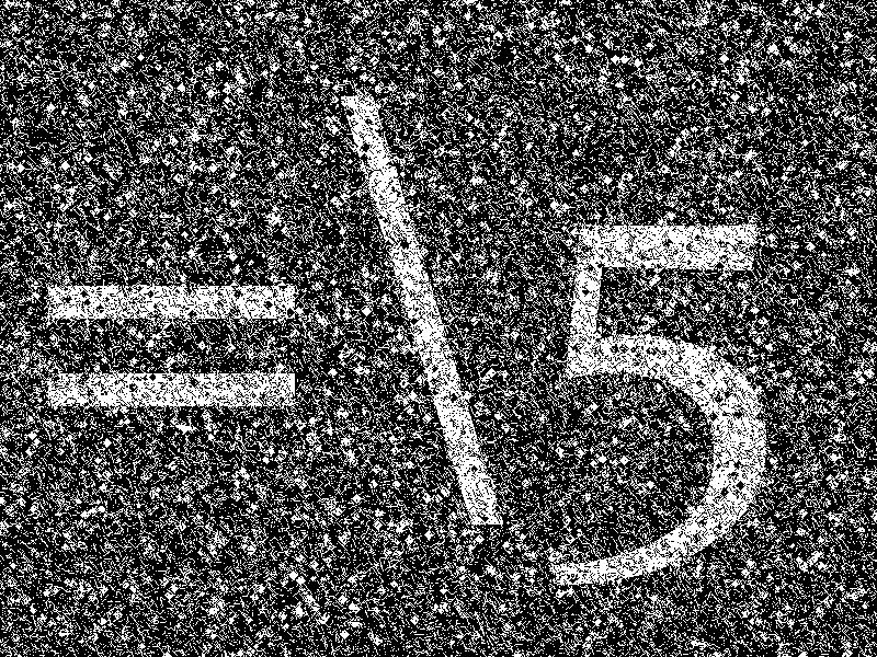
89 (a) (b) (c) (d) (e) (f) (g) (h) (i) (j) (k) (l) (m) (n) (o) (p) (q) (r) (s) (t) Figure 4.15: Sixth dataset considered. Average M SE = 26.90%. 87

90 Figure 4.16: Error versus size of the filter for all sets of noisy images using the operator ASF c. Figure 4.17: Error versus size of the filter for all sets of noisy images using the operator ASF c. 88

91 ASF c ASF c Dataset Error (%) Size Error (%) Size Table 4.1: Summary of the best results of operators ASF c and ASF c datasets. for all ASF ch ASF ch Dataset Error (%) Size Error (%) Size / 2 Table 4.2: Summary of the best results of operators ASF ch and ASF ch all datasets. for erators ASF ch and ASF ch, respectively. The behaviour of the curves is very similar to the operators ASF c and ASF c, but with a faster decrease in the error value. However the minimum value of error obtained by the operator ASF ch is not as low as the values obtained by the operator ASF c. However, the operator ASF ch obtained better error values when compared to the operator ASF c. Table 4.2 shows the best error values obtained by the operators ASF ch and ASF ch for all six datasets. Figures 4.20 and 4.21 show the error versus size of the filter graph for the operators ASF cm and ASF cm for all six datasets. The results are very similar to the results obtained with the operators ASF ch and ASF ch. Similarly, the values obtained by the operator ASF cm are slightly worse than the results of operator ASF c, while the operator ASF cm performs slightly better than the operator ASF c. Table 4.3 shows the error values for the best results obtained with operators ASF cm and ASF cm for all datasets. Figure 4.22 shows the result of the operator ASF þ. For the sixth dataset, the one with most noise, the filter further degrades the image, stabilizing 89

92 Figure 4.18: Error versus size of the filter for all sets of noisy images using the operator ASF ch. Figure 4.19: Error versus size of the filter for all sets of noisy images using the operator ASF ch. 90

93 Figure 4.20: Error versus size of the filter for all sets of noisy images using the operator ASF cm. Figure 4.21: Error versus size of the filter for all sets of noisy images using the operator ASF cm. 91

94 ASF cm ASF cm Dataset Error (%) Size Error (%) Size / 3 Table 4.3: Summary of the best results of operators ASF cm and ASF cm all datasets. for ASF þ ASF þ Dataset Error (%) Size Error (%) Size Table 4.4: Summary of the best results of operators ASF þ and ASF þ datasets. for all with an error value of more than 35%. For the other datasets, the error value was decreased slowly, with one exception to the fifth dataset and size 1 that increased the error before decreasing. Even on the datasets with less noise, the error values were worse than the values obtained by the operator ASF c. On the other hand, the operator ASF þ, illustrated on figure 4.23, presented a behaviour similar to the operators ASF c, ASF ch and ASF cm, but with better error values. The error values of the best obtained results for the operators ASF þ and ASF þ are shown in table 4.4. As we did on the section 4.2, we also processed this set of images using the classical alternating sequential filter, with normal and triple resolution, and the graph ASF introduced by Cousty et. al. [15]. Figures 4.24, 4.25 and 4.26 show the error versus size of the filter graph for these filters. with the classical ASF using triple resolution obtaining the best error values. The best results obtained for each of these operators is shown on table 4.5. The classical ASF presented the same behaviour of the operator ASF þ for the sixth dataset, increasing the error value. Considering the classical ASF 92

95 Figure 4.22: Error versus size of the filter for all sets of noisy images using the operator ASF þ. Figure 4.23: Error versus size of the filter for all sets of noisy images using the operator ASF þ. 93

96 Figure 4.24: Error versus size of the filter for all sets of noisy images using the classic ASF operator. Figure 4.25: Error versus size of the filter for all sets of noisy images using the classic ASF operator and triple resolution. 94

97 Figure 4.26: Error versus size of the filter for all sets of noisy images using the graph ASF [15]. Classic Classic x3 Graph Dataset Error (%) Size Error (%) Size Error (%) Size / / / / / / / / / Table 4.5: Summary of the best results of the classic ASF operator, with normal and triple resolution, and the graph ASF [15] for all datasets. 95

98 with triple resolution, that is, each pixel is divided in nine pixels, without interpolation, the result was considerably better, with better error results than the graph ASF [15]. This was expected because the classical operator with triple resolution has three intermediary sizes and the graph ASF only two. The results of the operator ASF c, considering the sixth dataset, is shown on figure The results for the classical ASF with triple resolution, also for the sixth dataset, is shown on figure Based on the results presented in this section, we conclude that, for binary images containing objects and a great amount of smaller noise, our operator outperforms the operators presented in the literature. 96

99 (a) (b) (c) (d) (e) (f) (g) (h) (i) (j) (k) (l) (m) (n) (o) (p) (q) (r) (s) (t) Figure 4.27: Results of the operator ASF c 6 on the sixth dataset. Average MSE = 1.17%. 97

100 (a) (b) (c) (d) (e) (f) (g) (h) (i) (j) (k) (l) (m) (n) (o) (p) (q) (r) (s) (t) Figure 4.28: Results of the classical ASF with triple resolution and size 7 1 / 3 for the sixth dataset. Average MSE = 1.62%. 98