MASSACHUSETTS INSTITUTE OF TECHNOLOGY DEPARTMENT OF MECHANICAL ENGINEERING CAMBRIDGE, MASSACHUSETTS NUMERICAL FLUID MECHANICS FALL 2011

Transcription

1 MASSACHUSETTS INSTITUTE OF TECHNOLOGY DEPARTMENT OF MECHANICAL ENGINEERING CAMBRIDGE, MASSACHUSETTS NUMERICAL FLUID MECHANICS FALL 2011 QUIZ 2 The goals of this quiz 2 are to: (i) ask some general higher-level questions to ensure you understand broad concepts and are able to discuss such concepts and issues with others familiar with numerical fluid mechanics; (ii) show that you understand and can apply concepts, methods and schemes that you learned; and (iii), show that you are able to read numerical codes and recognize what they accomplish. Partial credit will be given to partial answers. Shorter Concept Questions Problem 1 (25 points) Please provide a brief answer to the following questions (a few words to a few sentences is enough, with or without a few equations depending on the question). a) Provide two limitations of the von Neumann stability analysis. b) Explain how the discretization error and order of accuracy can be estimated numerically, without knowing the true solution. If you find that the estimated order of accuracy is not as expected, what are three possible causes? c) You evaluate the stability of your advection scheme and you find that the Courant-Friedrichs-Lewy condition does not give you the same condition as a von Neumann stability analysis. Which of the two conditions are you going to utilize, if any? Why? d) Briefly state three advantages that Multistep methods have over Runge-Kutta methods and three advantages that Runge-Kutta methods have over Multistep methods. e) The effective wave speeds of numerical representations of advection schemes are usually smaller than the real wave speed and usually dependent on the wavenumber. Briefly explain what this implies for numerical simulations. f) A friend tells you that for your FV scheme, you should always initialize your solution by computing the integral of your initial conditions over each finite volume. Otherwise, she says, your nodal values will not represent the volume average over the cell. Another friend tells you that you can initialize with the initial conditions evaluated at the nodal centers and that you should not bother doing integrals since it will be within the truncation errors. Are both of your friends right or wrong, or is only one of them right? Briefly explain why. g) To simulate a turbulent pipe flow systems with bends and corners, your friend recommends a non-orthogonal shape-following finite-volume grid, with a staggered pressure and velocity arrangements, specifically: pressure at nodal points and Cartesian-coordinate velocities at the boundaries of these pressure finite-volumes. Is this a good idea or not? Briefly explain why. Solution Notes: Some of the answers provided are much more complete than required for full credit. a) Some of the limitations of the von Neumann stability analysis are that in the theoretical sense, it only applies only to periodic BC problems and to linear problems (with constant coefficients). It also assumes that errors can be represented as Fourier series. b) The discretization error and order of accuracy can be estimated numerically, without knowing the true solution, by computing three and two solutions on systematically refined/coarsened grids, p respectively. The true solution u can be expressed either as u u x x R, or p uu2 x '(2 x) R' or u u4 '' (2 ) p x x R''. Assuming the three s and R s are similar, one eliminates u, the s and the R s to obtain: - 1 -

2 u - With three solutions: 2x u 4x p log log 2 u x u2 x u - With two solutions (assuming p is known): x u2x x p 2 1 If the estimated order of accuracy is not as expected, possible causes are: a bug in the code; the finitedifference scheme is not stable (e.g. a CFL condition is not satisfied for some of the solutions); the discretization of the boundary conditions are not of the same order as the order of the interior finitedifferences; the initial and/or boundary conditions are such that nonlinear terms and derivatives are (locally) significant; the resolution is too coarse (for the truncation error term to behave as ( ) ˆ p x x( ) O( x ) for x0); the (linear)-system solver does not converge (or is not applicable) and/or the system is poorly conditioned; the grid refinement is not systematic in complex geometrical cases; or, the round-off errors amplify (which is often less frequent than the other cases). c) If when evaluating the stability of an advection scheme, you find that the CFL condition does not give the same condition as a von Neumann stability analysis, you would utilize the stricter of the two since neither is always sufficient. However, it is very likely that the stricter of the two is the von Neumann condition since it often provides a sufficient condition for stability (in addition to always providing a necessary condition). A von Neumann condition is thus often more restrictive than a CFL condition. However, if the CFL is more restrictive, then one would use the CFL. In general, in multidimensional and multi-scale problems, one may also utilize a combination of (local) stability conditions. This is because: i) different terms in the PDEs can dominate the solution locally (in time or space) and, ii) estimating a stability condition valid everywhere in the domain, for all initial and boundary conditions, is not often feasible in such complex cases. d) To integrate over [t n+1, t n ], advantages of Multistep methods include: i) only one new RHS is needed at each time step; ii) accuracy is increased by adding points at previous time steps (at which the solution and so the RHS have already been computed), hence they are less expensive for a given order than RK methods (RKs are more expensive since the n th order RK requires n evaluations of the RHS, the 1 st derivative); iii) smaller stencils are needed for implicit multistep schemes (only values at t n+1 needed); iv) stores RHS/solutions only at chosen time-steps (not at intermediate steps); iv) can be easier to code. Advantages of RK methods include: i) for a given order, RK methods are more accurate and more stable than multistep methods of same order; ii) high-order multistep methods use derivatives that could be irrelevant to what is going on during [t n+1, t n ] (RKs use derivatives within [t n+1, t n ], a reason why RKs are more stable); iii) RKs are directly started but it is more difficult to start Multistep methods; and, iv) Multistep methods require storing old solutions (at past time steps). e) Since effective wave speeds of numerical representations of advection schemes are usually smaller than the real wave speed and usually dependent on the wavenumber, numerical simulations will lead to waves that travel a slower speeds than in reality and will numerically disperse a given wave (introduce other frequencies). f) Both friends can be right or wrong. If one initializes the solution by computing the integral of the ICs over each FV, the nodal values will represent the volume average over the cell and everything will be consistent. However, if the FV scheme is 2 nd order (e.g. mi-point rule is employed for integrals), then you could initialize with the ICs evaluated at the nodal centers since the mid-point value is equal to the integral-average over the cell at second order, hence differences will be within the truncation errors. Note we assumed in both cases that FVs are cell centered and FVs are sufficiently refined. g) To simulate a turbulent pipe flow systems with bends and corners, the idea of a non-orthogonal shape-following finite-volume grid, with a staggered pressure and velocity arrangements, and pressure at nodal points is good. However, if you utilize Cartesian-coordinate velocities at the boundaries of these pressure finite-volumes, this is likely to lead to velocities that are (quasi)-parallel to the edges some of the FVs. These FVs would be very ill posed: i.e. large variations in velocities and their errors would lead to small variations in the fluxes and their errors, and vice-versa

3 Idealized Computational Problems Problem 2: Local Stability of a Numerical Scheme (30 points) Consider the following one-dimensional temperature diffusion, 2 T T 2 t x and its discretization, n1 n n1 n1 n1 n n n Tj T j Tj 1 2Tj Tj 1 Tj 12Tj T j1 (1 ) 2 2 with0 1 t x x t and define r. 2 x a) Determine the leading term of the local truncation error in terms of r, and temperature derivatives at time n and point j. What are the orders of accuracy of the discretized equation in time and in space? b) Using your result in a) provide an expression for * () r that maximizes these orders of accuracy in time and space for a given r. What are these maximum orders of accuracy? c) Using a von Neumann stability analysis, determine the stability criterion for the discretized equation. 1 1 d) Based on your results in c), discuss 4 cases: 0,, and 1, expressing in 2 2 each case the stability conditions on r. Relate your results to the forward Euler (classic explicit), backward Euler (classic implicit) and Crank-Nicolson schemes. e) How does the cost of the scheme obtained in b) with * () r compare to that of the Crank-Nicolson scheme? f) Using your von Neumann analysis in c-d), provide a condition which guarantees no oscillation of the errors and a condition which guarantees constant signs for discrete temperatures (and their errors). Very briefly discuss the results. g) If you were to utilize the above discretization to determine the steady state temperature, which range of values for would you choose? Why? Can you utilize any values for r? - 3 -

4

5

6

7

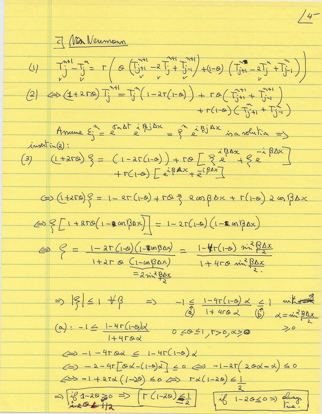
8

9

10

11 Problem 3: Finite Volumes on Triangles. (25 points) Consider the conservative form of a partial differential equation governing the two-dimensional (2D) in space advection-diffusion-reaction of a variable per unit volume (a surface in 2D):.( v).( ) s n t A finite-volume discretization is employed to solve this equation numerically, using equilateral triangles over the given domain. A representative triangle is illustrated on Figure 1: triangles have sides of length L and are fixed in time and space. The finite-volume discretization is node-centered for. Velocities are staggered and defined normal and outward to the edges of each triangle. a) Utilizing a mid-point rule for the surface (volume) integrals, provide the spatial discretization of the time-rate of change term and of the source term for the center triangle P. b) Discretize the convective fluxes for the center triangle P, using a mid-point rule for W sw n w s P n S e n E se Figure 1. Representative equilateral triangle, with center node P and sides of length L. The center nodes of the west, east and south triangles are denoted as W, E and S, respectively. the edge integral and linear interpolation to estimate the center edge values in terms of nodal values. c) Discretize the diffusive fluxes for the center triangle P, using a mid-point rule for the edge integral and linear interpolation of fluxes (centered difference) to estimate the center edge fluxes in terms of nodal values. d) For the given discretizations, do you need to resolve flux discontinuities in b) and/or c) to ensure conservative flux discretizations? If yes, please do so. If not, explain why. e) Combining a)-d), write the resulting finite-volume discretization for center triangle P. f) Should the triangle not be equilateral, what would be the order of accuracy of the spatial discretization obtained in e)? What is the main reason for this result? - 4 -

12 Solution: Consider the integral form of the governing differential equation (Integrate over the control volume V):.( v).( ) s t dv.( v) dv.( ) dv s dv t We are asked to evaluate each of these terms individually using different interpolations and approximations. a. (5 points) Time rate of change term (using a midpoint rule to evaluate volume integrals): d dp T1 dv dv PdV V t t dt dt The control volume in our case is the shaded equilateral triangle of side length L and unit thickness normal to the plane. The area of this equilateral triangle is given by: 3 2 A L 4 Therefore, 3 2 V L 4 We finally, have the approximate spatial discretization of the time rate of change term as: 3 d 2 P T1 L 4 dt The source term is also handled in a similar manner: This gives: T S dv S dv VS 4 P P T4 L S P b. (5 points) The convective term and the diffusive term are a little more complicated to deal with. Convective flux: T2.( v) dv - 5 -

13 Using Gauss theorem, the above volume integral can be transformed into a surface integral as follows: T dv v nds 2.( v). Using a linear interpolation for edge centered values and a mid-point rule for the surface integral, the above expression reduces to: T v. nds L v. n 2 int Since the control volume has three edges, the above term will have three different contributions. e P E 1. Edge n-se: T2 v. nds Lev. n Lve 2 w P W 2. Edge n-sw: T2 v. nds Lwv. n Lvw 2 s P S 3. Edge sw-se: T2 v. nds Lsv. n Lvs 2 Finally, we get: P S P W P E T2 Lvs Lvw Lve c. (5 points) Diffusive Fluxes: These fluxes are handled similar to advective fluxes. We have, T dv nds 3.( ). Using midpoint rule for the edge integrals and linear interpolation for edge centered values we get: d T3. nds L dn Since the CV has three edges, we again get three different contributions to the diffusive fluxes. e d E P 1. Edge n-se: T3 L L 3 E P dn L 3 2 w T 2. Edge n-sw: 3 3 W P s 3. Edge sw-se: T Finally, we get: 3 3 S P - 6 -

14 T3 3 E P 3 W P 3 S P d. (4 points) The advective and diffusive fluxes at the edge of a CV are exactly equal and opposite to the fluxes at the same edge due to the neighboring CV. This means that when the integral form of the equation is solved in the entire domain, the interior fluxes cancel out. Therefore, there is no flux discontinuity at the boundaries of neighboring CVs. e. (2 points) Putting every term of the integral form together, we have the following governing equation: f. (4 points) 3 2 dp P S P W P E L Lvs Lvw Lve 4 dt E P 3W P 3S P LS P 4 When the triangles are not equilateral, the discretization will no longer be second order accurate. This is because the normals from adjacent triangles will not line up in the same direction. When the triangles are equilateral, the cell centers are equidistant, due to which, the first order term in the Taylor series expansion cancels out. This leaves only the second order term as the leading term in the truncation error. When the triangles have different sizes, the centers are no longer equidistant from each other and this leads to a scheme which is only first order accurate

15 Problem 4: Code for solving a PDE (20 points) The MATLAB code for solving a PDE is given below: % MATLAB Code for solving a PDE. clear all,clc,clf, close all; % Initialize constants Nx=21; % Number of grid points x=1; % Length of domain dx=x/(nx-1); % Grid spacing Nt=601; % Total number of time steps t=1; % Final time dt=t/(nt-1); % Time step c=0.5; C = c*dt/(2*dx); % Initial conditions for i=1:nx if (dx*(i-1) >0.5) u(i,1)=1; else u(i,1)=0; end end % Fill in Matrix H: H = zeros(size(u,1),size(u,1)); for ii=3:size(u,1) H(ii,ii) = 1+3*C; H(ii,ii-1) = -4*C; H(ii,ii-2) = C; end H(1,1) = 1+3*C; H(1,end) = -4*C; H(1,end-1) = C; H(2,1) = -4*C; H(2,2) = 1+3*C; H(2,end) = C; % Fill in Matrix L; L=diag(ones(1,Nx)); for i=2:nx-1 L(i,i-1)=-C; L(i,i+1)= C; end L(1,2) = C;L(1,end) = -C; L(end,1) = C;L(end,end-1) = -C; L = inv(l); % Time integration for k = 2:Nt uold = L*u(:,k-1); unew = zeros(nx,1); iter=0; while(norm(unew-uold)>0.0001) if (iter~=0) uold = unew; end - 8 -

16 unew = L*u(:,k-1) + (eye(nx)-l*h)*uold; iter=iter+1; end u(:,k)=unew; end u_dc = u; Answer the following questions: a) Which equation is being solved by the given MATLAB code? What are the initial conditions? What type of boundary condition is implemented? b) Which types of discretization in space and time do the L and H matrices correspond to? c) Which scheme is being implemented in the code? d) Give two reasons why one would want to use this scheme. Solution: a. (6 points) The equation being solved in this code is the Sommerfeld wave equation. u u c 0 t x The initial conditions are as follows: Periodic boundary conditions are implemented. ux ( 0.5) 0 ux ( 0.5) 1 b. (5 points) The L matrix stands for the coefficient matrix obtained by discretizing the equation using a backward difference in time and a central difference in space. You can see this by looking at the structure of the L matrix. It is tri diagonal with minor modifications at the top-right and bottomleft of the matrix to incorporate the periodic boundary conditions. H matrix is obtained by discretizing the equation by using a backward difference in time and a second order backward difference in space. The idea is to call them Lower (L) and Higher (H) because we want to solve the equation without having to invert H, which can possibly be dense. c. (5 points) The scheme implemented in the code is a deferred correction approach. It is an iterative scheme using which one obtains the solution of a higher order method without actually having to invert a large coefficient matrix. Using the solution of a lower order scheme, one can iteratively update the solution until the solution becomes higher order accurate

17 d. (4 points) The main reasons one would use a deferred correction approach is: 1. Reduce oscillations in the solution 2. Avoid inversion of a large H matrix

18 MIT OpenCourseWare Numerical Fluid Mechanics Fall 2011 For information about citing these materials or our Terms of Use, visit: