Solution Methods. Steady State Diffusion Equation. Lecture 04

Transcription

1 Solution Methods Steady State Diffusion Equation Lecture 04 1

2 Solution methods Focus on finite volume method. Background of finite volume method. Discretization example. General solution method. Convergence. Accuracy and numerical diffusion. Pressure velocity coupling. Segregated versus coupled solver methods. Multigrid solver. Summary.

3 Overview of numerical methods Many CFD techniques exist. The most common in commercially available CFD programs are: The finite volume method has the broadest applicability (~80%). Finite element (~15%). Here we will focus on the finite volume method. There are certainly many other approaches (5%), including: Finite difference method (FDM). Finite element method (FEM). Spectral method. Boundary element method (BEM). Vorticity based methods. Lattice gas/lattice Boltzmann. And more!

4 Finite difference method (FDM) Historically, the oldest of the three. Techniques published as early as 1910 by L. F. Richardson. Seminal paper by Courant, Fredrichson and Lewy (1928) derived stability criteria for explicit time stepping. First ever numerical solution: flow over a circular cylinder by Thom (1933). Scientific American article by Harlow and Fromm (1965) clearly and publicly expresses the idea of computer experiments for the first time and CFD is born!! Advantage: easy to implement. Disadvantages: restricted to simple grids and does not conserve momentum, energy, and mass on coarse grids. 4

5 Finite difference: basic methodology The domain is discretized into a series of grid points. A structured (ijk) mesh is required. The governing equations (in differential form) are discretized (converted to algebraic form). First and second derivatives are approximated by truncated Taylor series expansions. The resulting set of linear algebraic equations is solved either iteratively or simultaneously.

6 Taylor Series: central finite difference method Subtract: Central difference formula 2 nd order accurate

7 Finite element method (FEM) Earliest use was by Courant (1943) for solving a torsion problem. Clough (1960) gave the method its name. Method was refined greatly in the 60 s and 70 s, mostly for analyzing structural mechanics problem. FEM analysis of fluid flow was developed in the mid- to late 70 s. Advantages: highest accuracy on coarse grids. Excellent for diffusion dominated problems (viscous flow) and viscous, free surface problems. Disadvantages: slow for large problems and not well suited for turbulent flow.

8 Finite volume method (FVM) First well-documented use was by Evans and Harlow (1957) at Los Alamos and Gentry, Martin and Daley (1966). Advantage: Was attractive because while variables may not be continuously differentiable across shocks and other discontinuities; mass, momentum and energy are always conserved. FVM enjoys an advantage in memory use and speed for very large problems, higher speed flows, turbulent flows, and source term dominated flows (like combustion). Late 70 s, early 80 s saw development of body-fitted grids. By early 90 s, unstructured grid methods had appeared. Advantages: basic FV control volume balance does not limit cell shape; mass, momentum, energy conserved even on coarse grids; efficient, iterative solvers well developed. Disadvantages: false diffusion when simple numerics are used. 7

9 Finite volume: basic methodology Divide the domain into control volumes. Integrate the differential equation over the control volume and apply the divergence theorem. To evaluate derivative terms, values at the control volume faces are needed: have to make an assumption about how the value varies. Result is a set of linear algebraic equations: one for each control volume. Solve iteratively or simultaneously.

10 Cells and nodes Using finite volume method, the solution domain is subdivided into a finite number of small control volumes (cells) by a grid. The grid defines the boundaries of the control volumes while the computational node lies at the center of the control volume. The advantage of FVM is that the integral conservation is satisfied exactly over the control volume. 9

11 Typical control volume The net flux through the control volume boundary is the sum of integrals over the four control volume faces (six in 3D). The control volumes do not overlap. The value of the integrand is not available at the control volume faces and is determined by interpolation. 10

12 The Finite Volume Method for Diffusion Problems

13 Finite Volume method Consider the 1D diffusion (conduction) equation with source term S Another form, where is the diffusion coefficient and S is the source term. Boundary values of at points A and B are prescribed. An example of this type of process, one-dimensional heat conduction in a rod.

14 Step 1: Grid generation The first step in the finite volume method is to divide the domain into discrete control volumes. Place a number of nodal points in the space between A and B. The boundaries (or faces) of control volumes are positioned mid-way between adjacent nodes. Thus each node is surrounded by a control volume or cell. It is common practice to set up control volumes near the edge of the domain in such a way that the physical boundaries coincide with the control volume boundaries. A general nodal point is identified by P and its neighbours in a one-dimensional geometry, the nodes to the west and east, are identified by W and E respectively. The west side face of the control volume is referred to by 'w' and the east side control volume face by e. The distances between the nodes W and P, and between nodes P and E, are identified by x WP and x PE respectively. Similarly the distances between face w and point P and between P and face e are denoted by x wp and x Pe The control volume width is x = x we

15 Step 2: Discretisation The key step of the finite volume method is the integration of the governing equation (or equations) over a control volume to yield a discretised equation at its nodal point P. Integrate over the control volume, from west to east face = 0 Here A is the cross-sectional area of the control volume face, V is the volume and S is the average value of source S over the control volume. It is a very attractive feature of the finite volume method that the discretised equation has a clear physical interpretation. Above equation states that the diffusive flux of leaving the east face minus the diffusive flux of entering the west face is equal to the generation of, i.e. it constitutes a balance equation for over the control volume.

16 Step 2: Discretisation In order to derive useful forms of the discretised equations, the interface diffusion coefficient and the gradient d /dx at east ( e ) and west ('w') are required. The values of the property and the diffusion coefficient are defined and evaluated at nodal points. To calculate gradients (and hence fluxes) at the control volume faces an approximate distribution of properties between nodal points is used. Linear approximations seem to be the obvious and simplest way of calculating interface values and the gradients. This practice is called central differencing. In a uniform grid linearly interpolated values for e and w are given by And the diffusive flux terms are evaluated as

17 Step 2: Discretisation In practical situations, the source term S may be a function of the dependent variable. In such cases the finite volume method approximates the source term by means of a linear form: Therefore, equation become Rearranging, Identifying the coefficients of W and E as A W and A E and the coefficient of P as A P, the above equation can be written as Where, Discretised form of diffusion equation

18 Step 3: Solution of equations Discretised equations of the form above must be set up at each of the nodal points in order to solve a problem. For control volumes that are adjacent to the domain boundaries the general discretised equation above is modified to incorporate boundary conditions. The resulting system of linear algebraic equations is then solved to obtain the distribution of the property at nodal points. Any suitable matrix solution technique may be used Matrix result into tridiagonal systems. TDMA is used.

19 Worked examples: one-dimensional steady state diffusion Consider the problem of source-free heat conduction in an insulated rod whose ends are maintained at constant temperatures of 100 C and 500 C respectively. The onedimensional problem sketched in figure below is governed by equation given below. Calculate the steady state temperature distribution in the rod using Finite Volume Method and compare the results with exact analytical solution. Thermal conductivity k equals 1000 W/m/K, cross-sectional area A is 10 x 10-3 m 2, use dx = 0.1 m (1)

20 Solution Divide the length of the rod into five equal control volumes as shown in Figure below. This gives dx = 0.1 m. The grid consists of five nodes. For each one of nodes 2, 3 and 4 temperature values to the east and west are available as nodal values. Consequently, discretised equations can be readily written for control volumes surrounding these nodes: The thermal conductivity (k e = k w = k), node spacing ( x) and cross-sectional area (A e = A W = A) are constants. Therefore the discretised equation for nodal points 2, 3 and 4 is

21 Solution With, S U and S P are zero in this case since there is no source term in the governing equation Nodes 1 and 5 are boundary nodes, and therefore require special attention. Integration of equation (1) over the control volume surrounding point 1 gives (2) Re-arrange, (3)

22 Solution Comparing equation 3 with equation 4 it can be easily identified that the fixed temperature boundary condition enters the calculation as a source term (S U + S P T P ) with S U = (2kA/ x)t A and Sp = -2kA/ x and that the link to the (west) boundary side has been suppressed by setting coefficient a W to zero. (4) (3) Equation 3 may be cast in the same linear form to yield the discretised equation for boundary node 1: With,

23 Solution The control volume surrounding node 5 can be treated in a similar manner. Its discretised equation is given by Re-arrange, The discretised equation for boundary node 5 is Where,

24 Solution The discretisation process has yielded one equation for each of the nodal points 1 to 5. Substitution of numerical values gives ka/ x = 100 and the coefficients of each discretised equation can easily be worked out. Their values are given in Table The resulting set of algebraic equations for this example is

25 Solution This set of equations can be re-arranged as For T A = 100 and T B = 500 the solution can obtained by using, for example, Gaussian elimination: The exact solution is a linear distribution between the specified boundary temperatures: T = 800x Figure shows that the exact solution and the numerical results coincide.

26 Solution

27 Assignment 5 Page 92, CFD Book by Versteeg Heat conduction with source term Figure shows a large plate of thickness L = 2 cm with constant thermal conductivity k = 0.5 W/m/K and uniform heat generation q = 1000 kw/m 3. The faces A and B are at temperatures of 100 C and 200 C respectively. Assuming that the dimensions in the y- and z-directions are so large that temperature gradients are significant in the x-direction only, calculate the steady state temperature distribution using Finite volume Method. Compare the numerical result with the analytical solution. The governing equation is 1. Solve for 5, 10 and 15 nodes 2. Compare the results

28 Assignment 6 Shown in Figure below is a cylindrical fin with uniform cross-sectional area A. The base is at a temperature of 100 C (Tb) and the end is insulated. The fin is exposed to an ambient temperature of 20 C. One-dimensional heat transfer in this situation is governed by where h is the convective heat transfer coefficient, P the perimeter, k the thermal conductivity of the material and T the ambient temperature. Calculate the temperature distribution along the fin and compare the results with the analytical solution given by where n 2 = hp/(ka), L is the length of the fin and x the distance along the fin. Data: L = 1 m, hp/{ka) = 25 m -2 (note ka is constant). Solve for 5, 10 and 15 nodes Compare the results

29 Finite volume method for two-dimensional diffusion problems The methodology used in deriving discretised equations in the one-dimensional case can be easily extended to two-dimensional problems. Two-dimensional grid used for the discretisation

30 Finite volume method for two-dimensional diffusion problems When the above equation is integrated over the control volume we obtain (5) As before this equation represents the balance of the generation of in a control volume and the fluxes through its cell faces. Using the approximations we can write expressions for the flux through control volume faces:

31 Finite volume method for two-dimensional diffusion problems By substituting the above expressions into equation 5 we obtain When the source term is represented in linearised form S V = S U + S P P, the equation can be re-arranged as

32 Finite volume method for two-dimensional diffusion problems Above equation is now cast in the general discretised equation form for interior nodes: Where,

33 Finite volume method for two-dimensional diffusion problems We obtain the distribution of the property in a given two-dimensional situation by writing above discretised equations at each grid node of the subdivided domain. At the boundaries where the temperatures or fluxes are known the discretised equations are modified to incorporate boundary conditions. The boundary side coefficient is set to zero (cutting the link with the boundary) and the flux crossing the boundary is introduced as a source which is appended to any existing S U and S P terms. Subsequently, the resulting set of equations is solved to obtain the twodimensional distribution of the property.

34 Finite volume method for three-dimensional diffusion problems Steady state diffusion in a three-dimensional situation is governed by A cell or control volume in three dimensions and neighboring nodes

35 Finite volume method for three-dimensional diffusion problems Integration of equation above over the control volume shown gives Putting the values at control faces (as in 2D case), we have

36 Finite volume method for three-dimensional diffusion problems Rearranging the coefficients, we have: where Boundary conditions can be introduced by cutting links with the appropriate face(s) and modifying the source term as described earlier

37 General approach In the previous example we saw how the species transport equation could be discretized as a linear equation that can be solved iteratively for all cells in the domain. This is the general approach to solving partial differential equations used in CFD. It is done for all conserved variables (momentum, species, energy, etc.). For the conservation equation for variable φ, the following steps are taken: Integration of conservation equation in each cell. Calculation of face values in terms of cell-centered values. Collection of like terms. The result is the following discretization equation (with nb denoting cell neighbors of cell P):

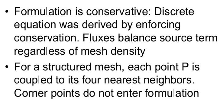
38 Guiding Principles Freedom of choice gives rise to a variety of discretization. As the number of grid points increased, all formulations are expected to give the same solution. However, an additional requirements is imposed that will enable us to narrow down the number of acceptable formulations. We shall require that even the coarse grid solution should always have Physically realistic behavior Overall balance

39 Guiding Principles Physically realistic behavior A realistic behavior should have the same qualitative trend as the exact variation Example: In heat conduction without source no temperature can lie outside the range of temperature established by the boundary temperature Conservation The requirement of overall balance implies integral conservation over the whole calculation domain heat flux, mass flow rates, momentum fluxes must correctly be balanced in overall for any grid size- not just for a finer grid Constraint Constraint of physical realism and overall balance will be used to guide our choices of profile assumptions and related practices-on the basis of these practice we will develop some basic rule that will enable us to discriminate between available formulations and to invent new ones

40 Four Basic Rules-(1/4) Consistency at control volume faces-same flux expression at the faces common to neighboring CVs

41 Four Basic Rules-(2/4) All coefficients must have same sign say positive. Implies that if neighbor goes up, P also goes up If an increase in E must lead to an increase in P, it follows that a E and a P must have same sign

42 Four Basic Rules-(2/4) But there are numerous formulations that frequently violates this rule. Usually, the consequence is a physically unrealistic solution. The presence of a negative neighbor coefficient can lead to the situation in which an increase in a boundary temperature causes the temperature at the adjacent grid point to decrease.

43 Four Basic Rules-(3/4)

44 Four Basic Rules-(4/4)

45 Four Basic Rules-(4/4)

46 End