FHWA-SC Form DOT F (8-72) Technical Report Documentation Page 2. Government Accession No. 3. Recipient's Catalog No. 1. Report No.

Transcription

1 1. Report No. FHWA-SC Technical Report Documentation Page 2. Government Accession No. 3. Recipient's Catalog No. 4. Title and Subtitle Guide for Estimating the Dynamic Properties of South Carolina Soils for Ground Response Analysis 5. Report Date November 13, Performing Organization Code 7. Author(s) Ronald D. Andrus, Jianfeng Zhang, Brian S. Ellis, and C. Hsein Juang 9. Performing Organization Name and Address Clemson University Civil Engineering Department Clemson, SC Sponsoring Agency Name and Address South Carolina Department of Transportation P. O. Box 191 Columbia, SC Performing Organization Report No. 10. Work Unit No. (TRAIS) 11. Contract or Grant No. SC-DOT Research Project No Type of Report and Period Covered Final Report March 14, 2001 to Nov. 13, Sponsoring Agency Code 15. Supplementary Notes 16. Abstract South Carolina is the second most seismically active region in the eastern U.S. The 1886 Charleston earthquake caused about 60 deaths and an estimated $23 million (1886 dollars) in damage. An important step in the engineering design of new and the retrofit of existing structures in earthquakeprone regions is the prediction of strong ground motions. Required inputs for ground response analysis include the small-strain shear wave velocity, the variation of normalized shear modulus with shear strain, and the variation of material damping ratio with shear strain for each soil layer beneath the site in question. Collectively, these inputs are known as the dynamic soil properties. This report presents guidelines for estimating the dynamic properties of South Carolina soils for ground response analysis. Regression equations for estimating small-strain shear-wave velocity from CPT and SPT data are presented in this guide. The regression equations are based on findings in previous studies and 123 penetration-velocity data pairs from South Carolina. Variables in the CPT-velocity equations are: cone tip resistance, soil behavior type index, depth, and geology. In the SPT-velocity equations, variables are: corrected blow count, fines content, depth, and geology. Shear-wave velocity measurements in Pleistocene soils are 20 % to 30 % greater than velocity measurements in Holocene soils with the same penetration resistance. In Tertiary soils, shear-wave velocity measurements are 40 % to 130 % greater than velocity measurements in Holocene soils with the same penetration resistance, and appear to depend on the amount of carbonate in the soils. (Continued) 17. Key Word Cone penetration test; earthquakes; ground motion; material damping; resonant column test; shear modulus; shear-wave velocity; site effects; South Carolina; standard penetration test; surface geology; torsional shear test 19. Security Classif. (of this report) Unclassified 20. Security Classif. (of this page) Unclassified 18. Distribution Statement 21. No. of Pages Price Form DOT F (8-72) Reproduction of completed page authorized

2 16. Abstract (Continued). Predictive equations for estimating normalized shear modulus and material damping ratio are also presented. They are based on a modified hyperbolic model and test results from Resonant Column and Torsional Shear tests on 122 samples. Input variables in the predictive equation for normalized shear modulus are: strain amplitude, confining stress, plasticity index (PI), and geology. In general, the recommended normalized shear modulus curve for Holocene soils with PI = 0 follows the Seed et al. upper range curve for sand, the Idriss curve for sand, and the Stokoe et al. curve for sand. On the other hand, the recommended normalized shear modulus curves for the older soils with PI = 0 generally follow the Seed et al. mean or lower range curves for sand and the Vucetic and Dobry curve for PI = 0 soil. The material damping ratio curves are expressed in terms of normalized shear modulus and minimum material damping ratio. Relationships between minimum damping and PI are developed based only on Torsional Shear test data. In general, the recommended damping curve for Holocene soils with PI = 0 follows the Seed et al. lower range curve for sand and the Idriss curve for sand and clay. The recommended damping curves for the older soils with PI = 0 generally follow the Seed et al. mean curve for sand and the Vucetic and Dobry curve for PI = 0 soils. Additional penetration-velocity data are needed from older soils, particularly the residual soils and saprolites in the Piedmont and natural sediments in the Middle and Upper Coastal Plain. Additional normalized shear modulus and material damping ratio data are needed from all deposit types in South Carolina, particularly the Lower Coastal Plain. The guidelines serve as a resource document for practitioners and researchers involved in predicting ground motions in the southeastern U.S. Form DOT F (8-72) Reproduction of completed page authorized

3 Guide for Estimating the Dynamic Properties of South Carolina Soils for Ground Response Analysis Sponsored by the South Carolina Department of Transportation Final Report November 13, 2003 By: Ronald D. Andrus, Ph.D., Jianfeng Zhang, Brian S. Ellis, and C. Hsein Juang, Ph.D., P.E. Department of Civil Engineering Lowry Hall, Box (864) Department of Civil Engineering College of Engineering and Science Clemson University Clemson, South Carolina USA

4

5 ACKNOWLEDGMENTS The South Carolina Department of Transportation (SCDOT) and the Federal Highway Administration (FHWA) funded this work under SCDOT Research Project No Their support is sincerely appreciated. The implementation committee for this project included: Timothy N. Adams, Lucero E. Mesa, Michael R. Sanders, Jeffery C. Sizemore, Terry L. Swygert, and Eduardo A. Tavera of SCDOT. The authors also thank the many individuals and organizations that generously provided data considered in the development of this guide. Special thanks to: Timothy N. Adams Roy H. Bordon Randy Bowers William M. Camp Ethan Cargill Mark M. Carter Thomas J. Casey Sanjoy Chakraborty Timothy J. Cleary Benjamin Forman Sarah L. Gassman Jack B. Phillips Glenn J. Rix Clay Sams Frank Syms Joseph Wang David Wilson William B. Wright Doug Wyatt SCDOT North Carolina State University South Carolina State Ports Authority S&ME, Inc. S&ME, Inc. Santee Cooper Wright Padgett Christopher Wilbur Smith Associates Gregg In Situ U.S. Army Corps of Engineers, Savannah District University of South Carolina U.S. Army Corps of Engineers, Savannah District Georgia Institute of Technology LawGibbs Bechtel Savannah River, Inc. Parsons-Brinckerhoff Geotrack Technologies, Inc. (formerly with Trigon Engineering Consultants) Wright Padgett Christopher Bechtel Savannah River, Inc. Finally, the authors thank the staff at Clemson University for their administrative support of this project. The following students assisted with compiling the data: Nicolas Giacomini, Russell Charles, and Cedric Fairbanks. v

6 vi

7 TABLE OF CONTENTS ACKNOWLEDGMENTS... TABLE OF CONTENTS... LIST OF TABLES... v vii xi LIST OF FIGURES... xv CHAPTER 1 INTRODUCTION BACKGROUND PURPOSE REPORT OVERVIEW... 5 CHAPTER 2 ESTIMATING IN SITU SHEAR-WAVE VELOCITY FROM PENETRATION DATA DATA FROM SOUTH CAROLINA General Characteristics of the Compiled Data Standard Penetration Test Blow Count Cone Penetration Test Tip and Sleeve Resistances Shear-Wave Velocity CPT-VELOCITY EQUATIONS Earlier Equations for Holocene-Age Soils Recommended Equations for South Carolina Sands SPT-VELOCITY EQUATIONS Earlier Equations for Holocene-Age Soils Recommended Equations for South Carolina Sands SUMMARY vii

8 CHAPTER 3 ESTIMATING NORMALIZED SHEAR MODULUS AND MATERIAL DAMPING RATIO FROM SITE CHARACTERISTICS FACTORS AFFECTING NORMALIZED SHEAR MODULUS AND MATERIAL DAMPING RATIO LABORATORY DATA FROM SOUTH CAROLINA AND SURROUNDING STATES NORMALIZED SHEAR MODULUS Earlier General Curves Recommended Values of γ r and α for South Carolina Soils Comparison of Recommended and Earlier General Curves MATERIAL DAMPING RATIO Earlier General Curves Recommended Values of D min and f(g/g max ) for South Carolina Soils Comparison of Recommended and Earlier General Curves SUMMARY CHAPTER 4 APPLICATION OF THE RECOMMENDED PROCEDURES FOR ESTIMATING THE DYNAMIC PROPERTIES OF SOUTH CAROLINA SOILS NEW COOPER RIVER BRIDGE AND EXAMPLE SITE PREDICTED SHEAR-WAVE VELOCITY FROM CPT DATA Age Scaling Factor Soil Behavior Type Index Predicted and Design V S PREDICTED G/G max FROM SITE CHARACTERISTICS PREDICTED DAMPING FROM SITE CHARACTERISTICS SUMMARY CHAPTER 5 SUMMARY AND RECOMMENDATIONS SUMMARY FUTURE STUDIES APPENDIX A REFERENCES viii

9 APPENDIX B SYMBOLS AND NOTATION APPENDIX C SUMMARY OF FIELD V S, CPT AND SPT DATA FROM SOUTH CAROLINA COMPILED FOR THIS STUDY APPENDIX D SELECTED PENETRATION-VELOCITY EQUATIONS FROM EARLIER STUDIES APPENDIX E SUMMARY OF CPT-V S AND SPT-V S REGRESSION EQUATIONS DEVELOPED FOR THIS STUDY APPENDIX F SUMMARY OF COMPILED LABORATORY SHEAR MODULUS AND MATERIAL DAMPING DATA FROM SOUTH CAROLINA AND SURROUNDING STATES ix

10 x

11 LIST OF TABLES Table Page 2.1 Site and references of field data used to develop the penetration-velocity predictive equations Corrections to SPT (modified from Skempton, 1986) as listed by Robertson and Wride (1998) Boundaries of soil behavior type and zones (after Robertson, 1990) Recommended CPT-V S equations for use in ground response studies in South Carolina Age scaling factors and statistical characteristics for the recommended CPT-V S equations SPT-V S equations by Piratheepan and Andrus (2002) recommended for use in ground response studies in South Carolina Age scaling factors and statistical characteristics for the recommended SPT-V S equations Relative importance of various factors on G/G max and D of soils (after Darendeli, 2001) Sites and references of laboratory data the G/G max and D predictive equations Recommended values of γ r1, α, k and D min1 for South Carolina soils Generalized soil/rock model for the DS-1 site, new Cooper River Bridge Design values of γ r, α, k and D min for the DS-1 site C.1 Summary of shear-wave velocity and penetration test data xi

12 Table Page C.2 Summary of characteristics of the selected layer D.1 Selected earlier SPT-V S equations proposed for Holocene sands D.2 Selected earlier CPT-V S equations proposed for Holocene sands D.3 Selected earlier CPT-V S equations proposed for Holocene clays D.4 Selected earlier CPT-V S equations proposed for all Holocene soils E.1 Developed CPT-V S regression equations based on measurements in all Holocene soil types and from South Carolina, California, Canada, and Japan E.2 Developed CPT-V S regression equations based on measurements in sandy and clayey Holocene soils and from South Carolina, California, Canada, and Japan E.3 Developed CPT-V S regression equations based on stress-corrected measurements Holocene soils and from South Carolina, California, Canada, and Japan E.4 Selected CPT-V S regression equations based on uncorrected measurements Holocene soils with calculated age scaling factors for Pleistocene soils in the South Carolina Coastal Plain E.5 Selected CPT-V S regression equations based on uncorrected measurements Holocene soils with calculated age scaling factors for all Tertiary soils in the South Carolina Coastal Plain E.6 Selected CPT-V S regression equations based on uncorrected measurements Holocene soils with calculated age scaling factors for Tertiary soils in the South Carolina Coastal Plain grouped by geologic formation E.7 Selected CPT-V S regression equations based on stress-corrected measurements Holocene soils with calculated age scaling factors for Pleistocene and Tertiary soils in the South Carolina Coastal Plain grouped by geologic formation xii

13 Table Page E.8 Selected SPT-V S regression equations developed by Piratheepan and Andrus (2002) with reported s and R 2 values for Holocene soils from California, Japan and Canada grouped by fines content E.9 Selected SPT-V S regression equations developed by Piratheepan and Andrus (2002) for Holocene soils with calculated age scaling factors for Pleistocene soils in the South Carolina Coastal Plain E.10 Selected SPT-V S regression equations developed by Piratheepan and Andrus (2002) for Holocene soils with calculated age scaling factors for Teriary soils in the South Carolina Coastal Plain E.11 Example calculations of age scaling factor (ASF) and residual standard deviation (s) F.1 Dynamic laboratory test samples from Charleston, South Carolina F.2 Dynamic laboratory test samples from Savannah River Site, South Carolina F.3 Dynamic laboratory test samples from Richard B. Russell Dam, South Carolina F.4 Dynamic laboratory test samples from North Carolina F.5 Dynamic laboratory test samples from Opelika, Alabama xiii

14 xiv

15 LIST OF FIGURES Figure Page 1.1 Stress-strain curve showing G max and G Typical normalized shear modulus reduction curve Hysteresis loop for one cycle of loading Typical relationship between material damping ratio and shear strain Map of South Carolina showing general locations of V S and penetration test sites for the compiled data Characteristics of the compiled penetration-v S data from South Carolina Normalized CPT soil behavior type chart by Robertson (1990) Simplified CPT soil behavior type chart (modified from Robertson, 1990) with data compiled for this study grouped by USCS soil type Simplified CPT soil behavior type chart (modified from Robertson, 1990) with data compiled for this study grouped by geologic age Comparison of q c versus V S measurements from South Carolina grouped by providing organization and inferred geologic age Comparison of earlier CPT-V S1 equations for Holocene sandy soils along with data from Holocene soils with I c < Comparison of earlier CPT-V S equations for Holocene clayey soils along with data from Holocene soils with I c > Comparison of measured and predicted V S as a function of q c, I c, and depth for Holocene data primarily from South Carolina and California xv

16 Figure Page 2.10 Comparison of the recommended CPT-V S relationship for Holocene soils and data primarily from South Carolina and California Comparison of measured and predicted V S as a function of q c, I c, and depth for Pleistocene data from South Carolina Comparison of the recommended CPT-V S relationship for Pleistocene soils and data from South Carolina Comparison of measured and predicted V S as a function of q c, I c, and depth for Tertiary data from South Carolina Comparison of the recommended CPT-V S relationship for Tertiary soils and data from South Carolina Comparison of N 60 versus V S measurements from South Carolina grouped by providing organization and inferred geologic age Comparison of earlier SPT-V S equations for Holocene sandy soils Comparison of earlier SPT-V S1 equations for Holocene sandy soils along with data from soils with FC = 10 % to 33 % Comparison of measured and predicted V S as a function of N 60 for data from South Carolina with fines content less than 40 % Comparison of the recommended SPT-V S relationships with the compiled data Map of South Carolina showing general sample locations for compiled dynamic laboratory test data Characterisitics of the complied dynamic laboratory data Comparison of selected earlier general normalized shear modulus curves Comparison of measured and predicted G/G max for the compiled data xvi

17 Figure Page 3.5 Comparison of compiled data and recommended G/G max log γ curves for Holocene-age soils with curves proposed by Vucetic and Dobry (1991) Comparison of compiled data and recommended G/G max log γ curves for Pleistocene-age soils with curves proposed by Vucetic and Dobry (1991) Comparison of compiled data and recommended G/G max log γ curves for the Tertiary-age Ashley Formation and stiff Upland soils with curves proposed by Vucetic and Dobry (1991) Comparison of compiled data and recommended G/G max log γ curves for all Tertiary-age soils at SRS except stiff Upland soils with curves proposed by Vucetic and Dobry (1991) Comparison of compiled data and recommended G/G max log γ curves for Piedmont residual soils with curves proposed by Vucetic and Dobry (1991) Comparison of selected earlier general material damping ratio curves Relationship between D min1 and PI based on TS test results by UTA Relationship between G/G max and D minus D min Comparison of measured and predicted D for the compiled data Comparison of compiled data and recommended D log γ curves for Holoceneage soils with curves proposed by Vucetic and Dobry (1991) Comparison of compiled data and recommended D log γ curves for Pleistocene-age soils with curves proposed by Vucetic and Dobry (1991) Comparison of compiled data and recommended D log γ curves for the Tertiary-age Ashley Formation and stiff Upland soils with curves proposed by Vucetic and Dobry (1991) xvii

18 Figure Page 3.17 Comparison of compiled data and recommended D log γ curves for all Tertiary-age soils at SRS except the stiff Upland soils with curves proposed by Vucetic and Dobry (1991) Comparison of compiled data and recommended D log γ curves for Piedmont residual soils with curves proposed by Vucetic and Dobry (1991) Seismic CPT measurements from the DS-1 investigation site, new Cooper River Bridge (S&ME, 2000) Predicted V S from CPT measurements at DS Comparison of measured and predicted V S profiles for the DS-1 site Base design (a) normalized shear modulus and (b) material damping ratio curves for the Holocene and Pleistocene soils at the DS-1 site Base design (a) normalized shear modulus and (b) material damping ratio curves for the Ashley Formation at the DS-1 site Base design (a) normalized shear modulus and (b) material damping ratio curves for soils beneath the Ashley Formation at the DS-1 site xviii

19 CHAPTER 1 INTRODUCTION 1.1 BACKGROUND Earthquake hazards are a major concern for the state of South Carolina. The 1886 Charleston earthquake (moment magnitude, M w 7.3) was the strongest historic earthquake to occur in the eastern U. S., causing about 60 deaths and an estimated $23 million (1886 dollars) in damage. Paleoliquefaction evidence suggests that at least five other large earthquakes have occurred in South Carolina during the last 2000 to 5000 years (Obermier et al., 1985; Talwani and Cox, 1985; Amick and Gelinas, 1991). In a recent study by Talwani and Schaeffer (2001), they estimate the earthquakes prior to 1886 near Charleston occurred about and years ago. This evidence has lead the U. S. Geological Survey (Frankel et al., 2000; to map significantly higher expected ground shaking levels than indicated on previous maps for South Carolina. Thus, future large earthquakes in the state are expected, and property damage during these future events will likely exceed several billion dollars (FEMA, 2000). Required inputs for earthquake ground motion and site response analysis include stiffness and material damping information for each soil layer at the site in question. Soil stiffness is represented by either shear-wave velocity or shear modulus. Small-strain shearwave velocity, V S, is directly related to small-strain shear modulus, G max, by: 2 max = S (1.1) G ρv where ρ is the mass density of soil (total unit weight of the soil divided by the acceleration of gravity). Illustrated in Figure 1.1 is the relationship between G max, shear strain, γ, and shear stress, τ. At moderate to high strains, the secant modulus, G, is used to represent the average stiffness. It is common in engineering practice to normalize G by dividing by G max. A plot showing the variation of G/G max with shear strain is called a normalized modulus reduction curve, and is illustrated in Figure

20 Shear Stress, τ 1 G max 1 τ G = γ Shear Strain, γ Figure 1.1 Stress-strain curve showing G max and G. 1.0 Normalized Shear Modulus, G/Gmax Shear Strain, γ, % Figure 1.2 Typical normalized shear modulus reduction curve. 2

21 Material damping ratio, D, represents the energy dissipated by the soil and is related to the stress-strain hysteresis loops generated during cyclic loading. Mechanisms that contribute to material damping are friction between soil particles, strain rate effect, and nonlinear soil behavior. Hysteretic damping can be defined by: W D = D (1.2) 4πWS where W D is the energy dissipated in one cycle of loading, and W S is the maximum strain energy stored during the cycle. A hysteresis loop is shown in Figure 1.3. The area inside the loop is W D. The area of the triangle is W S. A typical curve representing the variation of material damping with shear strain for soil is illustrated in Figure 1.4. Theoretically, there should be no dissipation of energy at the linear elastic behavior stage. However, even at very low strain levels, there is always some energy dissipation measured in the laboratory testing and the material damping ratio of soils never goes to zero. In the linear range, the damping ratio is a constant value and is referred to as the small-strain material damping, D min. At higher strains, nonlinearity in the stress-strain relationship (see Figure 1.1) leads to an increase in material damping with increasing strain amplitude. The field V S, the shear modulus reduction curve, and the damping versus shear strain curve are collectively referred in this document as the dynamic soil properties that are required for earthquake ground motion and site response analysis. 1.2 PURPOSE The current state of practice for determining the dynamic soil properties for ground response analysis involves 1) measuring or estimating the field V S, and 2) measuring or estimating the modulus reduction and material damping versus strain curves. While good direct measurements are always preferred, it is often not economically feasible to make these measurements for all locations and soil layers. In addition, measurements for the modulus reduction and damping curves are particularly expensive to make, and are usually made for only critical projects. This guide addresses the need for procedures for estimating the dynamic properties of soils in South Carolina that can be used to improve current earthquake ground motion and site response maps of the state, as well as provide inputs for site-specific response analysis. The procedures recommended in this guide are based on a review of earlier general procedures proposed for soils worldwide and a statistical analysis of existing data. 3

22 Shear Stress, τ 1 τ G = γ W S Shear Strain, γ W D WD D = 4πW S Figure 1.3 Hysteresis loop for one cycle of loading. 20 Material Damping Ratio, D, % D min Shear Strain, γ, % Figure 1.4 Typical relationship between material damping ratio and shear strain. 4

23 1.3 REPORT OVERVIEW Following this introduction, procedures for estimating V S from penetration measurements are discussed in Chapter 2. Procedures for estimating the variation of G/G max and material damping with shear strain are discussed in Chapter 3. In Chapter 4, an application of the recommended procedures using a case study from the new Cooper River Bridge in Charleston, South Carolina is presented. And, in Chapter 5, the recommended procedures are summarized and issues that remain to be resolved are identified. Six appendixes are included to assist the reader, and to provide information used in the development of the guidelines. A list of references cited in the guidelines is presented in Appendix A. A list of Symbols and Notation is presented in Appendix B. The compiled field V S and penetration data from South Carolina are summarized in Appendix C. Selected earlier penetration-v S equations are summarized in Appendix D. Tables summarizing CPT-V S and SPT-V S regression equations derived for this study are presented in Appendix E. Finally, the compiled dynamic laboratory test data from South Carolina and surrounding states are summarized in Appendix F. 5

24 6

25 CHAPTER 2 ESTIMATING IN SITU SHEAR-WAVE VELOCITY FROM PENETRATION DATA Empirical equations for estimating the small-strain shear-wave velocity, V S, of South Carolina soils from the Cone Penetration Test (CPT) and Standard Penetration Test (SPT) are presented in this chapter. The equations are particularly useful for regional seismic ground response hazard mapping, where it is not economically feasible to measure V S at all desired locations. They may be also useful for preliminary site-specific response analysis. However, V S should be measured directly for final site-specific response analysis. The empirical equations are based on statistical analysis of existing field data from primarily South Carolina. 2.1 DATA FROM SOUTH CAROLINA The existing SPT blow counts, CPT tip and sleeve resistances, and V S measurements are compiled for this study from various published and unpublished sources. The general locations of V S and penetration test sites are shown on the map in Figure 2.1 and summarized in Table 2.1. From the compiled data, 123 penetration and V S data pairs from South Carolina soil deposits are obtained. A detailed listing of the 123 penetration-v S data pairs is given in Appendix C. The general criteria used for selecting the penetration-v S data pairs are as follows: 1) Measurements are from below the groundwater table where reasonable estimates of effective stress can be made. 2) Measurements are from thick, uniform soil layers identified using CPT measurements. A distinct advantage of the CPT is that a nearly continuous profile of penetration resistance is obtained for detailed soil layer determination. By requiring V S and penetration resistance data to be from only thick, uniform soil layers, scatter in the data due to soil variability is minimized. When no CPT measurements are available, exceptions to Criterion 2 are allowed if there are several V S and SPT measurements within the layer that follow a consistent trend. 3) Penetration test locations are within 6 m of velocity test locations. 4) At least two V S measurements, and the corresponding test intervals, are within the uniform layer. 5) Time history records used for V S determination exhibit easy-to-pick shear-wave arrivals. Thus, values of V S determined from difficult-to-pick wave arrivals are not used. When time history records are not available, exceptions to Criterion 5 are allowed if there are at least 3 V S measurements within the selected layer above 20 m, or at least 5 V S measurements below 20 m. 7

26 lueridgepiedmonupercoamidstadlelowlplacoastalplainercoastalplain# BFall Line W N E ins Savannah River Site tsavannah Georgetown Charleston km Beaufort Figure 2.1 Map of South Carolina showing general locations of V S and penetration test sites for data compiled for this study Table 2.1 Sites and references of field data used to develop the penetration-velocity predictive equations. Counties Site Reference Charleston Cooper River Bridge; Maybank S&ME ( ) Highway (SC Highway 700); Ashley Phosphate/I-26 Interchange Charleston, Berkeley, SC Highway 170; various areas WPC ( ) Beaufort, and Jasper; Savannah, Ga. Charleston and Georgetown Ten Mile Hill, Gapway, Sampit Talwani et al. (2002); Hu et al. (2002) Aiken and Barnwell Savannah River Site WSRC (2000) 8

27 2.1.1 General Characteristics of the Compiled Data Distributions of the compiled data pairs with respect to average measurement depth, depth to water table, soil type, and inferred geologic age are presented in Figure 2.2. Of the 123 data pairs, about 98 % correspond to average measurement depths less than 28 m (Figure 2.2a). These depths correspond to calculated average values of σ ' v ranging from 36 kpa to 343 kpa, with only 6 average values from the Savannah River Site exceeding 300 kpa. The thickness of the selected layer vary from 2 m to 18 m, with 70 % less than 7 m. Nearly all the data pairs are from sites where the water table is between the ground surface and a depth of 14 m (Figure 2.2b). The Unified Soil Classification System (USCS) soil type is known for 26 % of the data pairs, and ranges from clean sand to organic clay (Figure 2.2c). Concerning the inferred geologic age of the deposits, 17 % are Holocene in age (< 10,000 years), 42 % are Pleistocene in age (10,000 to 1.8 million years), 36 % are Tertiary in age (1.8 to 65 million years), and 5 % are of unknown age (Figure 2.2d). The geologic ages of the selected soil layers are inferred from information provided in reports, maps produced by the South Carolina Geological Survey and U.S. Geological Survey, and communications with the investigator(s). The majority of the Holocene data are from the Charleston area. The Pleistocene and Tertiary data are from the lower and upper coastal plain areas in South Carolina. For the Pleistocene data, the distinguishable formations are the Wando and Ten Mile Hill. For the Tertiary data, the distinguishable formations are the Ashley (locally known as the Cooper Marl) in Charleston, and the Tobacco Road and Dry Branch at the Savannah River site. The influence that geologic age and formation have on the SPT-V S and CPT-V S equations will be discussed later in this chapter Standard Penetration Test Blow Count As specified in ASTM D , the SPT involves driving a 51-mm (2.0-inch) outside diameter, split-barrel sampler 0.46 m (18 inches) into the ground using a kN (140-lb) hammer dropped from a height of 0.76 m (30 inches). The number of blows to penetration the last 0.3 m (12 inches) is called the blow count or N-value. One distinct advantage of the SPT is that it provides a sample. Because there are many variations of SPT equipment and procedures, it is recommended that the measured blow count (N m ) be corrected to reference test conditions by the following equation (Youd et al., 2001): N = N 60 mcecbcrcs (2.1) 9

28 10

29 where N 60 is the equipment-corrected blow count, C E is the correction for hammer energy ratio (ER), C B is the correction factor for borehole diameter, C R is the correction for rod length, and C S is the correction for samplers with or without liners. Approximate values for C E, C B, C R, and C S are listed in Table 2.2. An ER of 60 % is commonly assumed as the average for U.S. testing practice and a reference value for the energy correction (C E = ER/60). Youd et al. (2001) recommend that hammer energy measurements be made at each site where the SPT is used. Where energy measurements cannot be made, the values listed in Table 2.2 may be used to approximate C E. For this study, the corrections factors listed in Table 2.2 are generally used to correct the compiled N m values. Energy measurements reported for several SPT drill rigs employed during the new Cooper River Bridge field investigations are used directly to correct those data. Where no energy measurements were reported, the average values listed in Table 2.2 are assumed based on the type of hammer used. Detailed borehole diameter, rod length, and sampling method information are typically not included in the project reports. Therefore, additional information was requested from the engineer in charge. Based on the additional information provided by the engineer, reasonable assumptions are made. Estimates of borehole diameters ranged from 100 mm to 150 mm. Rod lengths are assumed equal to the measurement depth plus 1 m. The value of C S is assumed 1.0 for all measurements (i.e., all samplers are assumed to have a constant inside diameter of 34.9 mm). Table 2.2 Corrections to SPT (modified from Skempton, 1986) as listed by Robertson and Wride (1998). Factor Term Equipment Variable Correction Energy ratio C E Donut hammer Safety hammer Automatic-trip donut type hammer Borehole diameter C B mm 150 mm 200 mm Rod length C R <3 m 3-4 m 4-6 m 6-10 m m Sampling method C S Standard sampler Sampler without liners

30 For some applications, SPT blow counts are further corrected to a reference overburden stress using the following equation: ( N ) N60CN 1 = (2.2) 60 where the correction factor C N is commonly calculated by the following equation (Liao and Whitman, 1986): C N P ' a = σ v 0.5 (2.3) where σ ' v is the effective vertical or overburden stress, and P a is a reference stress of 100 kpa (or 1 atm). Equation 2.3 is an approximation to the original correction curve proposed by Seed and Idriss (1982), and is limited to a maximum value of 1.7. Youd et al. (2001) endorse the use of Equation 2.3 for overburden pressures up to 300 kpa. For pressures greater than 300 kpa, they recommend that Equation 2.3 not be applied Cone Penetration Test Tip and Sleeve Resistances As specified in ASTM D , the CPT consists of measuring the load on the tip of a cone with an apex angle of 60 o and the skin friction over a short length of rod above the tip during penetration through soil deposits. Tip and sleeve resistances are typically recorded every 1 cm, providing a nearly continuous profile of subsurface stratigraphy. In addition, other measurements such as pore pressure and V S can be made at the same time (Lunne et al., 1997). Because samples are usually not collected during cone testing, CPT data are grouped in this study using a simplified version of the soil behavior type chart developed by Robertson (1990) shown in Figure 2.3. The value on the vertical axis represents a dimensionless cone tip resistance (Q) defined by (Robertson and Wride, 1998): q c v Pa Q σ = P a σ ' v n (2.4) 12

31 Figure 2.3 Normalized CPT soil behavior type chart by Robertson (1990). Table 2.3 Boundaries of soil behavior type and zones (after Robertson, 1990). Zone Soil Behavior Type Soil Behavior Type Index I c 1 Sensitive, fine grained Organic soils--peats I c > Clays--silty clay to clay 2.95 < I c < Silt mixtures--clayey silt to silty clay 2.60 < I c < Sand mixtures--silty sand to sandy silt 2.05 < I c < Sands--clean sand to silty sand 1.31 < I c < Gravelly sand to sand I c < Very stiff sand to clayey sand* Very stiff, fine grained* *Heavily overconsolidated or cemented 13

32 where q c is the measured cone tip resistance, σ v is the total overburden stress in the same units as q c and P a, and n is an exponent ranging from 0.5 to 1.0. The value on the horizontal axis represents normalized friction ratio (F) defined by (Wroth, 1988): F = q c f s 100% σ v (2.5) where f s is the measured cone sleeve friction in the same units as q c. The boundaries separating soil behavior type zones 2 to 7 shown in Figure 2.3 can be approximated as concentric circles, with the radius of each circle, term the soil behavior type index (I c ) defined by: 2 2 [( 3.47 logq) + ( 1.22 log F ) ] 0. 5 I c = + (2.6) General soil behavior type descriptions and corresponding I c values for each zone are given in Table 2.3. To select the suitable value of n for Equation 2.4, the iterative procedure by Robertson and Wride (1998) is followed. The first step is to calculate I c assuming n = 1.0. If the I c calculated with n = 1.0 is greater than 2.6, then 1.0 is selected for n. If the calculated I c is less than 2.6, it is recalculated using n = 0.5. If the recalculated I c is less than 2.6, then 0.5 is selected for n and the recalculated I c is used to group the data. However, if the recalculated I c is greater than 2.6, I c is again recalculated using n = 0.7 for the final value to be used in grouping the data. A simplified version of the soil behavior type chart by Robertson (1990) is shown in Figure 2.4. The vertical axis of this simplified chart is based on normalized cone tip resistance expressed by (Robertson and Wride, 1998): q c1n q = P c a C Q q = P c a Pa σ ' v n (2.7) where q c1n is the normalized cone tip resistance. Similar to the SPT, a maximum value of C Q of 1.7 is applied at shallow depths. The parameter I c defining the radius of the circles plotted in Figure 2.4 is calculated using Equation 2.6. Also plotted in Figure 2.4 are the compiled data grouped by soil type, as determined by USCS. The chart accurately predicts the soil type for the plotted data, with 6 exceptions. 14

33 Normalized Cone Tip Resistance, q c1n CL,CH,OH 4 10 ML,MH 3 SM,SC SP,SW,SP-SM,SP-SC Normalized Friction Ratio, F (%) Figure 2.4 Simplified CPT soil behavior type chart (modified from Robertson, 1990) with data compiled for this study grouped by USCS soil type. Normalized Cone Tip Resistance, q c1n Holocene 3 Pleistocene Tertiary Normalized Friction Ratio, F (%) Figure 2.5 Simplified CPT soil behavior type chart (modified from Robertson, 1990) with data compiled for this study grouped by geologic age. 15

34 Dividing the zones 2 to 7 in the soil behavior type charts shown in Figures 2.3 and 2.4 is a normally consolidated region that trends diagonally downward from left to right. According to Robertson (1990), data plotting above the normally consolidated region tend to indicate soils that are over-consolidated and older. Below the normally consolidated region, soils generally tend to exhibit higher sensitivity. Plotted in the chart shown in Figure 2.5 are the compiled data grouped by inferred geologic age. It can be seen that many of the data from Holocene deposits plot within the normally consolidated region. However, there are several Holocene data points above the normally consolidated region. Also contrary to expected behavior, the data from Pleistocene and Tertiary deposits plot in all areas of the chart Shear-Wave Velocity The field V S can be measured by several seismic test methods including seismic crosshole, seismic downhole, seismic cone penetrometer (SCPT), suspension logger, and Spectral-Analysis-of-Surface-Waves (SASW). General reviews of these methods are given in Woods (1994) and Ishihara (1996). All of the V S measurements in the 123 penetration-v S data pairs compiled for this study were determined by the SCPT method and calculated by the psuedo-interval method (Pantel, 1981; Campanella and Stewart, 1992). Following the traditional procedures for correcting penetration resistance to a reference overburden stress, V S is often corrected using the following equation (Sykora, 1987; Robertson et al., 1992): V S1 = V S C vs = V S P ' a σ v 0.25 (2.8) where V S1 is the stress-corrected shear-wave velocity, and σ ' v and P a are in the same units. Similar to the equations for correcting penetration resistance, Equation 2.8 implicitly assumes a constant coefficient of earth pressure at rest, K ' 0. Also implicitly assumed is that V S is measured with both the directions of particle motion and wave propagation polarized along principal stress directions and that one of those directions is vertical (Stokoe et al., 1985). Similar to the SPT and CPT, a maximum value of C vs of 1.4 is applied at shallow depths (Andrus and Stokoe 2000). 16

35 2.2 CPT-VELOCITY EQUATIONS The CPT-V S equations are considered first because more CPT-V S data pairs are available than SPT-V S data pairs. All of the 123 penetration-v S data pairs from South Carolina include CPT measurements. The compiled data with known geologic age are plotted in Figure 2.6. The plotted data are grouped by the providing organization and geologic age. The providing organizations include: S&ME, Inc. (S&ME), University of South Carolina (USC), WrightPadgettChristopher (WPC), and Westinghouse Savannah River Company (WSRC). It can be seen in the figure that V S generally increases with age for a given cone tip resistance. Because the data from Holocene-age soils are limited, the recommended equations are based, in part, on the compiled data and, in part, on earlier CPT-V S studies Earlier Equations for Holocene-Age Soils The relationship between CPT resistances and V S has been studied since about 1983, as reviewed in Piratheepan and Andrus (2002). A listing of selected earlier equations for Holocene-age sands, clays, and all soils is given in Appendix D. For comparison, several of these equations are plotted in Figures 2.7 and 2.8. Also plotted are data from South Carolina, along with data from California and Japan compiled by Piratheepan and Andrus (2002). 17

36 18

37 In Figure 2.7, earlier equations based on normalized cone tip resistance, as well as data for Holocene-age sands, are plotted. There is good agreement between the data from California and Japan compiled by Piratheepan and Andrus (2002) and equations proposed by Robertson et al. (1992), Hegazy and Mayne (1995), Andrus et al. (1999), and Piratheepan and Andrus (2002). On the other hand, the relationships by Rix and Stokoe (1991) and Fear and Robertson (1995) plot significantly above most of the data and other proposed relationships. The relationship by Baldi et al. (1986) plots between these two groups. Also, 6 of the 7 data points for South Carolina plot on high side of the data compiled by Piratheepan and Andrus (2002). It is likely that aging processes increased the velocities associated with the South Carolina data, because they are from natural soil deposits where the geologic age could be early Holocene. In Figure 2.8, earlier equations based on uncorrect cone tip resistances, as well as data for Holocene-age clays, are plotted. The equation by Hegazy and Mayne (1995) indicates that f s is somewhat of a significant parameter. However, based on the regression analysis by Piratheepan and Andrus (2002) and this study, I c appears to be a more significant parameter than f s. Thus, the equation by Piratheepan and Andrus (2002) based on q c, f s, and I c is plotted. As noted in Figure 2.8, when I c is introduced into the regression equation the exponent on f s becomes very small (-0.004), indicating that most of the variability can be explained by q c and I c. The relationship by Hegazy and Mayne (1995) for clays appears to be most appropriate for soils with I c of about 3.3, which corresponds to silty clay to clay soil behavior according to Robertson s (1990) chart. The plotted data from South Carolina and California are in good agreement with the plotted equations. Based on this review, the significant variables affecting CPT-V S relationships are: cone tip resistance, confining stress (or depth), soil type (or I c ), and geologic age. Considering these variables and combining the data from South Carolina with data from California, Canada and Japan, several new regressions are derived (Ellis, 2003). These new regression equations are listed in Appendix E Recommended Equations for South Carolina Soils Listed in Table 2.4 are the recommended CPT-V S equations for use in ground response studies in South Carolina. These equations are based on regression analysis of Holocene data from South Carolina, California, Canada, and Japan. They are recommended because they include all the significant variables identified in the previous section. Also, they provide some of the highest values of coefficient of multiple determination and lowest values of residual standard deviation of the equations listed in Appendix E. Equations that predict uncorrected V S are preferred because it is V S, and not V S1, that is needed for ground response analysis. 19

38 Table 2.4 Recommended CPT-V S equations for use in ground response studies in South Carolina. Soil Behavior Type, I c Equation for Predicting V a S, m/s Equation All values V S c c = 4.63q I Z ASF 2.9 b < 2.05 VS = 8.27qc Ic Z ASF 2.10 c > 2.60 VS = 0.208qc Ic Z ASF 2.11 c a q c in kpa, and Z is depth in meters. b Equation 2.9 is the simplest equation recommended for estimating V S for all soil types. c Somewhat better predictions of V S may be obtained using Equations 2.10 and 2.11 for soils with I c < 2.05 and I c > 2.60, respectively. For 2.05 < I c < 2.60, use Equation 2.9. Table 2.5 Age scaling factors and statistical characteristics for the recommended CPT-V S equations Location and Geologic Age of Deposit Soil Behavior Type, I c Age Scaling Factor, ASF 2 R Residual Standard Deviation, s, m/s No. of Samples, j Range of V, m/s S South Carolina Coastal Plain Holocene All values < a a > a South Carolina Coastal Plain Pleistocene All values < b ---- b > b South Carolina Coastal Plain Tertiary-age Ashley Formation (or Cooper Marl ) All values a South Carolina Coastal Plain Tertiary-age Tobacco Road Formation All values > b b South Carolina Coastal Plain Tertiary-age Dry Branch Formation All values < b b a Data from California, Canada and Japan. b R 2 not calculated. 20

39 Age scaling factors and statistical characteristics for the recommended equations are given in Table 2.5. The age scaling factor (ASF) is an adjustment to the reference model (equations for Holocene soils) for use in the older aged soils. It is defined as the measured V S divided by the predicted V S using the equation for Holocene-age soils. The residual standard deviation (s) is defined as the square root of [ (measured V S predicted V S ) 2 ]/(j-2), where j is the number of samples. It reflects how much the data fluctuate from the developed equation. Example calculations of ASF and s are given in Table E.11 of Appendix E. The coefficient of multiple determination (R 2 ) is the ratio of the deviation due to regression to the total variation in the dependent variable, which is velocity. The closer R 2 is to 1, the more the regression equation is said to explain the total variation. Predictions of V S outside the ranges indicated in Table 2.5 should be used with greater care. A plot of measured and predicted V S for the Holocene data using Equation 2.9 with ASF = 1.0 is shown in Figure 2.9. It can be seen in the figure that the V S measurements compiled for this study and V S measurements compiled by Piratheepan and Andrus (2002) are equally well predicted by Equation 2.9. The value of s associated with the plotted data and Equation 2.9 is 25 m/s. Considering that soil variability also contributes to scatter in the data, this s value is not unreasonable for ground response analysis. Even good V S measurements generally have errors of 5 %. Somewhat better predictions of V S can be achieved using Equations 2.10 and 2.11 for soils with I c < 2.05 and I c > 2.6, respectively. Presented in Figure 2.10 is a direct comparison the Holocene CPT-V S data pairs and Equation 2.9, using the average depth of the measurements of 7 m. Despite the fact that two of the variables are fixed in the plotted curves (i.e., Z = 7 m and q c = values between 1.4 and 3.9), the plotted data compare will with the curves. Shown in Figure 2.11 is a plot of measured and predicted V S for the Pleistocene data using Equation 2.9 with ASF = The ASF value of 1.23 suggests that V S is, on average, 23 % higher in Pleistocene soils of the South Carolina Coastal Plain than in Holocene soils with similar cone resistances. A comparison of the Pleistocene CPT-V S data pairs and Equation 2.9 using the average depth for the measurements of 7 m is presented in Figure The value of s associated with the plotted data and Equation 2.9 is 37 m/s. An s value of 37 m/s is about 1.5 times as large as the value determined for the Holocene data, indicating greater fluctuation about the equation. When Equations 2.10 and 2.11 are considered, the values of ASF and s are similar to values associated with Equation

40 22

41 23

42 A plot of measured and predicted V S for the Tertiary data using Equation 2.9 is shown in Figure The calculated ASF values for the Ashley, Tobacco Road, and Dry Branch Formations are on the order of 2.29, 1.65 and 1.38, respectively. These values are significantly higher than ASF values calculated for the Pleistocene soils. They suggest that, on average, V S is 38 % to 129 % higher in Tertiary soils than in Holocene soils with similar cone resistances. Equation 2.9 is plotted in Figure 2.14 using average values of depth, ASF and I c for the Ashley and Dry Branch Formations. Also plotted in Figure 2.14 are the Tertiary data grouped by geologic age and I c. The fluctuation of the plotted data about Equation 2.9 is characterized with s values of 64, 48 and 32 for the Ashley, Tobacco Road and Dry Branch Formations, respectively. It is interesting to note that all three Tertiary formations are similar in age. The Ashley Formation dates at about 30 million years before present (Weems and Lemon, 1993; Raymond A. Christopher, personal communication, November 2002), and is a deep marine deposit with an overconsolidation ratio (OCR) of about 3 to 7 and a calcium carbonate content of 60 to 70 %. The Tobacco Road and Dry Branch Formations date at about 25 to 29.5 million years and 34 to 36 million years, respectively (Raymond A. Christopher, personal communication, November 2002). According to the description given in WSRC (2000), the Tobacco Road Formation is a shallow marine deposit with OCR of 1 to 3 and contains some calcium carbonate. The Dry Branch Formation is a near shore and bay deposit. It is characterized as having an OCR of 1 to 3 and consisting of primarily quartz sand. The higher OCR associated with the Ashley Formation only partially explains the higher ASF, because the Tobacco Road and Dry Branch Formations have similar OCR values but different ASF values. On the other hand, the concentration of carbonate might explain the difference in calculated values of ASF. The Ashley Formation, having the highest amount, has the largest ASF value; and the Dry Branch Formation, having the lowest amount, has the smallest ASF value. Calcium carbonate is relatively easy to dissolve and re-crystallize. Its presence often suggests at least some weak cementing of soil particles. Based on these observations, it is likely that ASF is also dependent on the concentration of natural cementing agents, such as calcium carbonate, in addition to age. 2.3 SPT-VELOCITY EQUATIONS Twenty-six SPT-V S data pairs from South Carolina are available for this study. The reason for this small number is because SPTs are usually not performed close to CPTs. Of the 26 data pairs, 1 is for Holocene sands, 6 are for Holocene clays, 9 are for Pleistocene soils, and 10 are for Tertiary soils. The compiled data are plotted in Figure The data are grouped by the providing organization and inferred geologic age. Similar to the CPT-V S data, it can be seen that V S generally increases with age for a given SPT blow count. Given the limited amount of data, the recommend equations are based primarily on earlier SPT-V S studies. 24

43 25

44 2.3.1 Earlier Equations for Holocene-Age Soils Several investigators have studied SPT-V S relationships, since about Most of the relationships are for sandy soils. Relationships for clays are not common, likely because the blow count in soft clay is close to zero. General reviews of the earlier relationships are given in Sykora (1987) and Piratheepan and Andrus (2002). A listing of selected equations for Holocene sands that consider both corrected blow count and confining stress (or depth) is given in Appendix D. For comparison, several of the equations are plotted in Figures 2.16 and Also plotted are data from South Carolina, California, Canada, and Japan. In Figure 2.16, earlier equations for Holocene sands based on energy-corrected SPT blow count and depth are plotted, using a depth value of 10 m. As can be seen in the figure, there is fairly good agreement between equations despite the fact that the equation by Ohta and Goto (1978) is based on field data from Japan and the equation by Piratheepan and Andrus (2002) is based on field data from primarily California. The effect of grain size is unclear, however. The Ohta and Goto (1978) curves suggest that V S increases with increasing grain size for a given blow count, although the fine sand and medium sand curves are not consistent with this trend. On the other hand, the Piratheepan and Andrus (2002) curves suggest that V S increases with increasing fines content for a given blow count. 26

45 27

46 In Figure 2.17, earlier equations for Holocene sands based on energy- and stresscorrected SPT blow count are compared graphically. Also plotted in the figure are data from South Carolina, California, Canada, and Japan soils with fines content of 10 % to 33 %. The relationships by Piratheepan and Andrus (2002), Andrus and Stokoe (2000), Fear and Robertson (1995) for Ottawa sand, and Yoshida et al. (1988) for fine sand compare well. On the other hand, the relationships by Seed et al. (1986) for granular soils, Yoshida et al. (1988) for fine to coarse sand, and Fear and Robertson (1995) for Alaska sand suggest higher values of V S1 than the other relationships for the same blow count. The plotted data from California, Canada and Japan were used by Piratheepan and Andrus (2002) to derive their relationship for soils with fines content of 10 % to 35 %. The one data point from South Carolina (with FC = 28 %) plots on the high side of the other data. It is interesting to note that the relationships by Piratheepan and Andrus (2002) plotted in Figures 2.16 and 2.17 are based on the same data set. Seed et al. (1986) derived their relationship by assuming the Ohta and Goto (1978) equation for sandy gravel, which would plot above the curve for coarse sand shown in Figure This observation suggests that the assumption made by Seed et al. (1986) resulted in a relationship that predicts V S (or G max ) on the high side for many Holocene soils. The relationships by Yoshida et al. (1988) are based on calibration chamber tests. Fear and Robertson (1995) described Alaska sand as tailings composed of large amount of carbonate shell material and suggested that the shell material significantly increased its compressibility, which resulted in lower penetration resistances. An alternative hypothesis is that the high concentration of carbonate resulted in a weakly cemented soil skeleton having significantly higher V S measurements. Predicting V S on the high side may not be the best approach for ground response analysis. Earthquake records and analytical studies indicate that soft, low V S, soil deposits subjected to low accelerations, less than about 0.4 g, can amplify the bedrock motion (Idriss, 1990). Thus, the relationships by Ohta and Goto (1978), Yoshida et al. (1988) for fine sand, Fear and Robertson (1995) for Ottawa sand, Andrus and Stokoe (2000), and Piratheepan and Andrus (2002) are suggested as better general equations for predicting V S in uncemented, Holocene-age sands. Using the equations proposed by Piratheepan and Andrus (2002) and the available data, age scaling factors are derived for various soils in the South Carolina Coastal Plain (Ellis, 2003). These age scaling factors along with the associated statistics are listed in Appendix E. 28

47 2.3.2 Recommended Equations for South Carolina Sands Listed in Table 2.6 are the recommended SPT-V S equations for use in ground response analyses. The recommended equations are those derived by Piratheepan and Andrus (2002) using data from Holocene soils in California, Canada, and Japan. These equations are recommended because they 1) include all the significant parameters identified in the previous section (i.e., blow count, depth, fines content, and geologic age), 2) provide some of the highest values of R 2 and lowest values of s for the compiled data (see Appendix E), 3) predict V S (and not V S1 ), the required parameter for ground response analysis, and 4) provide a reasonable fit for the two data pairs from South Carolina. In addition, the results of the regression analysis given in Appendix E show that equations based on uncorrected and stress-corrected have similar values of R 2 and s associated with them. Age scaling factors and statistical characteristics for the recommended SPT-V S equations are given in Table 2.7. Similar to the CPT-V S equations, the ASF is equal to 1.0 for Holocene soils. The computed ASF for the 8 Pleistocene SPT-V S data pairs and Equation 2.12 is 1.23, which is practically the same as the computed ASF for the Pleistocene CPT-V S data pairs (see Table 2.5). The age scaling factors listed for Tertiary soils are tentative and should be used cautiously, because they are based on few SPT-V S data pairs. It is possible that the age scaling factors listed in Table 2.5 for Tertiary soils may be more representative. Nevertheless, the limited data provide a greater ASF for the Ashley Formation than for the Dry Branch Formation. These findings generally agree with the CPT-V S age scaling factors and suggest that aging processes may affect both SPT blow count and CPT tip resistance similarly. Presented in Figure 2.18 is a comparison of measured and predicted V S for the SPT-V S data pairs from South Carolina. The two Holocene data points fall within 25 m/s of the measured=predicted line. This generally agrees with the s value of 16 m/s associated with Equation 12 and Holocene soils with fines content less than 40 % (see Table 2.7). The value of s associated with the plotted Pleistocene data plotted in Figure 2.18 is 50 m/s. These values of s are similar to s values calculated for the Holocene and Pleistocene CPT-V S data (see Table 2.5). Somewhat lower s values are expected if Equations 2.13 and 2.14 are used for soils with fines content < 10 % and %, respectively. Predictions of V S outside the ranges indicated in Table 2.7 should be used with greater care. Presented in Figure 2.19 is a direct comparison the SPT-V S data pairs and Equation 2.12, using the average depth of the measurements of 5 m, 15 m, or 18 m. It can be seen that the few data plot fairly well about the predicting curves. 29

48 Table 2.6 SPT-V S equations by Piratheepan and Andrus (2002) recommended for use in ground response studies in South Carolina. Fines Content, FC, % Equation for Predicting V a S, m/s < ( N ) Z ASF Equation V S = b V S = c < ( N ) Z ASF V S = c 10 to ( N ) Z ASF a N 60 in blows/0.3 meter, and Z is depth in meters. b Equation 2.12 is the simplest equation recommended for estimating V S for soils with FC < 40 %. c Somewhat better predictions may be obtained using Equations 2.13 and 2.14 for soils with FC < 10 % and FC = 10 % to 30 %, respectively. Table 2.7 Age scaling factors and statistical characteristics for the recommended SPT-V S equations Location and Geologic Age of Deposit Fines Content, FC, % Age Scaling Factor, ASF 2 R Residual Standard Deviation, s, m/s No. of Samples, j Range of V, m/s S South Carolina Coastal Plain Holocene < 40 < a a 16 a 15 a 81 a 25 a a a 10 to a 8 a 10 a a South Carolina Coastal Plain Pleistocene < 40 < b ---- b to c ---- b ---- d South Carolina Coastal Plain Tertiary-age Ashley Formation (or Cooper Marl ) < to c b 1.71 c ---- b ---- d d South Carolina Coastal Plain Tertiary-age Dry Branch Formation < to c b 1.48 c ---- b ---- d d a Data from California, Canada and Japan. b R 2 not calculated. c Tentative ASF based on few measurements. ASF based on CPT data may be more representative. d At least 3 data pairs or samples needed to calculate s. 30

49 31

50 2.4 SUMMARY Guidelines and procedures for estimating V S of South Carolina Coastal Plain soils from CPT and SPT data were presented in this chapter. The recommended procedure for estimating V S from CPT data can be summarized in the following five steps: 1. Identify the major geologic units beneath the site in question. This involves determining the approximate age (e.g., Holocene, Pleistocene, Tertiary) and/or formation of each major geologic unit. 2. Calculate the soil behavior type index for each measurement depth in the CPT profile following the iterative procedure described in Section If necessary, convert the CPT tip resistances and depths to kpa and meters, respectively. 4. Calculate V S for each measurement depth using Equation 2.9 and the appropriate age scaling factors listed in Table 2.5. Note that Equation 2.9 was the simplest regression equation recommended for all soil types. Somewhat better estimates of V S may be obtained using Equation 2.10 for I c < 2.05, Equation 2.9 for 2.05 < I c < 2.60, and Equation 2.11 for I c > Plot the profile of calculated V S values. At locations where V S measurements have been made in close proximity to CPT measurements, compare the measured and predicted values of V S to verify the accuracy of the CPT-V S equations and age scaling factors. The recommended procedure for estimating V S from SPT data can be summarized in the following five steps: 1. Identify the major geologic units beneath the site in question. This involves determining the approximate age and/or formation of each major geologic unit. 2. Determine the fines content for each measurement depth. 3. Correct the measured blow count, N m, to the equipment-correct blow count, N 60, for each measurement depth following the procedures summarized in Section

51 4. Calculate V S for each measurement depth using Equation 2.12 and the appropriate age scaling factors listed in Table 2.7. Note that Equation 2.12 was the simplest regression equation recommended for soils with fines content < 40 %. Somewhat better estimates of V S may be obtained using Equation 2.13 for soils with fines content < 10 %, and Equation 2.14 for soils with fines content between 10 and 35. Also, note that age scaling factors listed in Table 2.7 are tentative for the older formations because they are based on limited data. 5. Plot the profile of calculated V S values. At locations where V S measurements have been made in close proximity to SPT measurements, compare the measured and predicted values of V S to verify the accuracy of the SPT-V S equations and age scaling factors. Based on both CPT and SPT data, age scaling factors are 1.00 for Holocene soils and 1.2 to 1.3 for Pleistocene soils. For Tertiary soils, computed age scaling factors range from 1.4 to 2.3, and appear to depend on the amount of carbonate in the soil. Residual standard deviations for the recommended equations are about 15 m/s to 25 m/s for the Holocene soils, 40 m/s to 50 m/s for the Pleistocene soils, and 20 m/s to 60 m/s for the Tertiary soils. Greater care should be exercised with using the recommended equations outside the ranges of V S listed in Tables 2.5 and 2.7. More data are needed to further validate the recommended equations for South Carolina soils, particularly the SPT-V S equations. Additional data are needed before equations can be recommended for soils of the Piedmont physiographic province. 33

52 34

53 CHAPTER 3 ESTIMATING NORMALIZED SHEAR MODULUS AND MATERIAL DAMPING RATIO FROM SITE CHARACTERISTICS Equations for estimating normalized shear modulus and material damping ratio from site characteristics are presented in this chapter. The equations are particularly useful for regional seismic ground response hazard mapping and preliminary site-specific response analysis in South Carolina. They may also be useful for final site-specific response analysis of non-critical structures. For final site-specific analysis involving critical structures, however, direct measurements should be made. The recommended equations are based on a review of earlier relationships and a statistical analysis of available laboratory test data. 3.1 FACTORS AFFECTING NORMALIZED SHEAR MODULUS AND MATERIAL DAMPING RATIO Many studies have been conducted to characterize the factors that affect normalized shear modulus and material damping ratio of soils (e.g., Seed and Idriss, 1970; Hardin and Drnevich, 1972a; Lee and Finn, 1978; Zen et al., 1978; Iwasaki et al., 1978; Kokusho et al., 1982; Ni, 1987; Sun et al., 1988; Vucetic and Dobry, 1991; Ishibashi and Zhang, 1993; Stokoe et al., 1995; Rollins et al., 1998, Vucetic et al. 1998, Stokoe et al., 1999; Darendeli, 2001). A summary of the relative importance of various factors is given in Table 3.1. The most important factors that affect normalized shear modulus, G/G max, are: strain amplitude, confining pressure, and soil type and plasticity. Other factors that affect G/G max, but are of less importance, include: number of loading cycles, frequency of loading, over-consolidation ratio, void ratio, degree of saturation, and grain characteristics. In general, G/G max curves degrade more slowly with shear strain as confining pressure and plasticity index (PI) increase. Iwasaki et al. (1978) and Kokusho et al. (1982) found that lower plasticity soils are more affected by effective confining pressure than higher plasticity soils. Other studies like Ishibashi and Zhang (1993) and Stokoe et al. (1999) showed that G/G max decreases generally less with increasing shear strain as confining pressure increases. Concerning material damping ratio, D, the most important influencing factors are: strain amplitude, confining pressure, soil type and plasticity, number of loading cycles, and frequency of loading. With increase of confining pressure, D tends to decrease for all strain amplitudes. The effect of soil plasticity on D is complex, however. EPRI (1993), Stokoe et al. (1994) and Vucetic et al. (1998) found that values of small-strain damping, D min, increase with 35

54 increasing PI, while values of D at high strains decrease with increasing PI. Earlier studies like Seed et al. (1986) and Vucetic and Dobry (1991) did not show this complex effect of PI on damping. As explained by Stokoe et al. (1999), one problem with laboratory D measurements lies in the identification of equipment-related energy loss. This effect must be quantified and deducted from the measured values to obtain the correct D. In addition, it has been suggested that D should be measured at frequencies and number of loading cycles similar to those of the anticipated cyclic loadings, to account for the effects of these factors. Considerations for the most important factors affecting G/G max and D are made in the development of the predictive equations. Table 3.1 Relative importance of various factors on G/G max and D of soils (after Darendeli, 2001). Parameter Importance on G/G max Importance on D Strain Amplitude Very Important Very Important Confining Pressure Very Important Very Important Soil Type and Plasticity Very Important Very Important Number of Loading Cycles Less Important Very Important Frequency of Loading Less Important Important Over-Consolidation Ratio Less Important Less Important Void Ratio Less Important Less Important Degree of Saturation Less Important Less Important Grain Characteristics, Size, Shape, Gradation, Mineralogy Less Important Less Important 3.2 LABORATORY DATA FROM SOUTH CAROLINA AND SURROUNDING STATES The available laboratory G/G max and D data from South Carolina and surrounding states are compiled from various published and unpublished sources, as summarized in Table 3.2. They include Resonant Column (RC) and Torsional Shear (TS) test data for 78 samples taken from three general areas in South Carolina: Charleston, Savannah River Site (SRS), and Richard B. Russell Dam (RBRD). In addition, RC and TS data for 44 samples taken from North Carolina and Alabama are included in the database. Locations of the Charleston, SRS and RBRD areas are plotted on the map of South Carolina shown in Figure 3.1. Because of the extensive earthquake hazard study conducted at SRS, laboratory results for 64 RC and 15 TS tests are available from that area. Lesser amounts of test data are available from the other areas. Although Cyclic Triaxial test data are also available, they are not considered in this report because of equipment-related concerns raised during an earlier evaluation of the SRS data set (Stokoe et al., 1995; Lee, 1996). Test results for samples from Charleston are available 36

55 lueridgepiedmontupercoamidstadlelowlplacoastalplainercoastalplaintable 3.2 Sites and references of laboratory data used to develop the G/G max and D predictive equations. Location Physiographic Province No. of Tests Reference Charleston, SC- Mark Clark Expressway; Daniel Island Terminal Savannah River Site, SC Richard B. Russell Dam, SC Seven sites (A to G) sampled by the North Carolina Department of Transportation Spring Villa NGES, Opelika, Alabama Lower Coastal Plain Upper Coastal Plain Piedmont Piedmont Piedmont 6 RC 3 TS 64 RC 15 TS 8 RC 5 RC 27 TS 12 RC S&ME (1993, 1998) Stokoe et al. (1995); Lee (1996); Hwang (1997) USACE (1973, 1979) Borden et al. (1994, 1996) Hoyos and Macari (1999) # BFall Line W N E ns irichard B. Russell Dam: 8 RC Savannah River Site: 64 RC and 15 TS km Charleston: 6 RC and 3 TS Figure 3.1 Map of South Carolina showing general sample locations for compiled dynamic laboratory test data. 37

56 in tabular format. For samples from North Carolina, all shear modulus data and damping data for 5 RC and 3 TS tests are available in tabular format. Damping data for an additional 24 TS tests on samples from North Carolina are available in graphical form, but are difficult to read. Therefore, these data are not considered in this report. Test results for samples from other locations are read from plots of shear modulus and damping versus shear strain. Results for six deep samples from SRS are not used in this study because they do not follow the general trend displayed by other samples (Stokoe et al., 1995). A detailed listing of the laboratory data is given in Appendix F. General characteristics of the data are described below. The Charleston and SRS areas lie in the Lower Coastal Plain and Upper Coastal Plain, respectively (see Figure 3.1). The other three areas lie in the Piedmont physiographic province. The Coastal Plain physiographic province generally consists of soft Quaternary soils to relatively stiff Tertiary soils, with depth to hard rock increasing from near zero at the western boundary of the Upper Coastal Plain, called the Fall Line, to about 1 km at the coast (S&ME, 2000; Wheeler and Cramer, 2000). Above the Fall Line lie the Piedmont and Blue Ridge physiographic provinces (see Figure 3.1), which consist largely of shallow zones of residual soils and saprolites overlying hard rock. Distributions of the 122 test samples with respect to the organization performing the test, sample depth, plasticity index, and geologic unit are presented in Figure 3.2. As shown in Figure 3.2(a), the RC and TS tests were performed by eight different laboratories. Of the 122 test samples: 3 were tested by Fugro-McClelland, Inc. (Fugro), 22 by GEI Consultants, Inc. (GEI), 14 by Law Engineering and Environmental Services, Inc. (Law), 13 by Purdue University (Purdue), 8 by the U.S. Department of the Army, South Atlantic Division Laboratory (SADEN-FL), 18 by The University of Texas at Austin (UTA), 32 by the North Carolina State University at Raleigh (NCSU), and 12 by the Georgia Institute of Technology (GT). The test samples were collected from depths ranging from 0.6 m to 326 m. As shown in Figure 3.2(b), 50 % of the samples are from depths less than 10 m. About 72 % are from depths less than 30 m. Most samples were tested at mean confining pressures similar to the estimated in-situ mean effective confining pressures. Some were tested at several different confining pressure levels to reflect the confining pressure range that soils at the site were expected to experience. Values of PI are known for 101 of the 122 test samples, ranging from 0 to 132. As illustrated in Figure 3.2(c), non-plastic (PI = 0) samples make up at least 35 % of the compiled samples. At least 73 % of the samples have PI values less than 30. Only about 10 % of the samples have PI values greater than 30, with just one sample having PI greater than

57 (a) Test Performing Organization (b) Sample Depth (c) Plasticity Index (d) Geologic Unit Figure Characteristics of the compiled dynamic laboratory data. 39

58 Geologic unit distribution for the test samples is shown in Figure 3.2(d). Of the 122 test samples, 6 are Holocene in age, 2 are Pleistocene in age, and 66 are Tertiary in age or even older. The other 48 samples are from residual soils and saprolites. Residual soils are clay-rich earths that are the remains of completely weathered rock. Saprolites are highly decomposed rock without the clay accumulation. Generally, no parent rock structure can be found in residual soils, while saprolites retain the relict structure of the original rock but have soil texture. Among the 6 Holocene-age samples, 2 are from Charleston and 4 are from embankment soil at the RBRD site. Two of the Tertiary-age samples are from the Ashley Formation beneath Charleston. The 64 samples from SRS are from various formations of Tertiary age or older. Most test samples were described as undisturbed, except for three samples from SRS that were described as somewhat disturbed (see Appendix F). 3.3 NORMALIZED SHEAR MODULUS Earlier General Curves A comparison of selected earlier general normalized shear modulus curves is presented in Figure 3.3. As can be seen, the Vucetic and Dobry (1991) curve for PI = 0 soil is similar to the Seed et al. (1986) mean curve for sand. This similarity suggests that the Vucetic and Dobry (1991) curves may be applicable to both fine- and coarse-grained soils. The curve proposed by Idriss (1990) for sand is practically identical to the Seed et al. (1986) upper range curve for sand. The Idriss (1990) curve for clay lies close to the Vucetic and Dobry (1991) curve for PI = 50 soil. The curve by Stokoe et al. (1999) for PI = 0 soil and depths (Z) = m lies between the Seed et al. (1986) mean and upper range curves for sand, and their curve for PI = 2-26 soils and Z = m lies above the Seed et al. (1986) upper range curve for sand. Hardin and Drnevich (1972a and 1972b) made one of the early attempts to develop mathematical equations to predict the G/G max curve using a hyperbolic model. The hyperbolic model assumes that the stress-strain curve of soil under cyclic loading can be represented by a hyperbola asymptotic to the maximum shear stress, τ max, and is expressed as: 1 G / Gmax = (3.1) γ 1+ γ where γ is the shear strain, and γ r is the reference strain (= G max /τ max ). One limitation of Equation 3.1 is its poor fit to some laboratory measurements because it involves only one fitting parameter, γ r. r 40

59 Normalized Shear Modulus, G/Gmax Stokoe et al. (1999) PI = 2-36; Z = m Seed et al. (1986) Mean curve and range for sand Idriss (1990) Sand Idriss (1990) Clay Stokoe et al. (1999) Sand; PI = 0; Z = m Vucetic and Dobry (1991) PI = Shear Strain, γ, % Figure 3.3 Comparison of selected earlier general normalized shear modulus curves Predicted G/Gmax Holocene Pleistocene Tertiary Residual Soil and Saprolite Measured = Predicted Predicting Equation: 1 G / Gmax = 1 + γ / γ ( ) α r Measured G/G max Figure Comparison of measured and predicted G/G max for the compiled data. 41

60 Improved fits to laboratory test data can be obtained using a modified hyperbolic model expressed as (Stokoe et al., 1999): 1 G / Gmax = (3.2) α γ 1+ γ r where α is an exponent called the curvature coefficient. Darendelli (2001) proposed an average α value of for all soils. Equation 3.2 is adopted in this study to model the variation of G/G max with shear strain for South Carolina soils Recommended Values of γ r and α for South Carolina Soils Values of γ r and α that provide the best fits to Equation 3.2 are determined for each RC or TS test series. It is found that values of γ r can vary greatly from one geologic unit to another, and generally increase with increasing plasticity and effective confining pressure. Assuming α is independent of confining pressure, calculated values of α are 1.00 for soils in SRS, but vary considerably for soils in Charleston and in the Piedmont. Listed in Table 3.3 are reference strains at a mean effective confining pressure of 100 kpa, γ r1, and corresponding α for various geologic units and PI values. As noted in the table, some of these values have been extrapolated from the range of available laboratory data and should be used with greater care. For values of PI other than those listed, interpolation between listed values is acceptable. For converting values of γ r1 listed in Table 3.3 to mean effective confining pressures other than 100 kpa, the following relationship is suggested (Stokoe et al., 1995): γ r γ r1 ( σ' / P ) k = (3.3) where σ' m is the mean effective confining pressure at the depth in question in kpa, P a is a reference pressure of 100 kpa, and k is an exponent that varies with geologic formation and PI. Suggested values for k are also listed in Table 3.3. The mean effective pressure is calculated by: m a 1+ 2K σ ' = ' 0 m σ v (3.4) 3 where σ' v is the vertical effective pressure, and Κ' 0 is the coefficient of effective earth pressures at rest. The coefficient Κ' 0 is defined as the horizontal effective pressure, σ' h, divided by σ' v. Procedures for estimating Κ' 0 can be found in most soil mechanics textbooks. Based on evaluations of laboratory data and analytical studies, Stokoe et al. (1995) suggested that actual σ' m should be within ±50 % range of the estimated values. This suggestion is also supported by the fact that σ' m (or depth) has been largely ignored in the earlier general G/G max curves. 42

61 Table 3.3 Recommended values of γ r1, α, k and D min1 for South Carolina soils. 43 Geologic Unit (Formation) No. of Samples Holocene 6 Pleistocene (Wando) Tertiary (Ashley or Cooper Marl ) Tertiary (stiff Upland soils) Tertiary (All soils at SRS except stiff Upland soils) Location Variable Soil Plasticity Index, PI COV for Ln (γ r1 ) Charleston γ r1, % a -- and α a -- Richard B. k a -- Russell Dam D min1, % a -- γ r1, % α k D min1, % γ r1, % -- c a a α a a k a a D min1, % a,b 1.52 b 2.49 a,b Charleston 2 Charleston 2 50 Savannah River Site Savannah River Site γ r1, % a α a k a D min1, % a γ r1, % a % α a k a D min1, % a R 2 G/G max : Damping: G/G max : Damping: G/G max : Damping: G/G max : Damping: G/G max : Damping: a Tentative values; extrapolated from the range of available laboratory test data. b Approximate; no Torsional Shear damping measurements available. c Little or no data available.

62 Table 3.3 Recommended values of γ r1, α, k and D min1 for South Carolina soils (Cont d). 44 Geologic Unit (Formation) Tertiary (Tobacco Road, Snapp) Tertiary (soft Upland soils, Dry Branch, Santee, Warley Hill, Congaree) Residual Soil and Saprolite No. of Samples Location Savannah River Site Savannah River Site 48 Piedmont Variable Soil Plasticity Index, PI COV for Ln (γ r1 ) γ r1, % a -- c 11.7 % α a k a D min1, % a γ r1, % a % α a k a D min1, % a γ r1, % a % α a k a D min1, % 0.56 b 0.85 b 1.14 b 1.52 a,b R 2 G/G max : Damping: G/G max : Damping: G/G max : Damping: a Tentative values; extrapolated from the range of available laboratory test data. b Approximate; no Torsional Shear damping measurements available. c Little or no data available.

63 Values of G/G max predicted using Equations 3.2, 3.3, and 3.4 for the compiled data are compared with measured G/G max values in Figure 3.4. As noted in Table 3.3, calculated values of R 2 range from to One point to keep in mind when interpreting the R 2 values is that most of the data are concentrated between G/G max values from 0.8 to 1.0, where error is inherently small because of normalization. Thus, the R 2 values probably do not reflect the goodness-of-fit of the model at lower values of G/G max. Perhaps more weight should be assigned to the G/G max values smaller than 0.8. Nevertheless, the plotted data in Figure 3.4 are fairly evenly distributed about the Measured = Predicted line. For geologic units where enough data exist, statistical variability of the compiled data is also provided in Table 3.3 in terms of coefficient of variation (COV) for reference strain. COV is defined as the standard deviation divided by the mean value, and is a measure of relative dispersion. Values of γ r1 for a certain geologic unit are found to be log-normally distributed and the COV values presented in the table are for Ln (γ r1 ) Comparison of Recommended and Earlier General Curves In Figures 3.5 through 3.9, the recommended G/G max curves are grouped by geologic unit and compared with the Vucetic and Dobry (1991) curves. Only the recommended curves for σ' m of 100 kpa are shown for simplicity. Also shown in these figures are the compiled laboratory test data, which are converted to equivalent values with σ' m = 100 kpa here through the correction of γ r using Equations 3.3. In Figure 3.5, the recommended curves for Holocene-age soils in Charleston and at RBRD are shown. As can be seen, the recommended curves for PI = 0 to 100 soils span a range narrower than the corresponding Vucetic and Dobry (1991) curves. The recommended curve for PI = 0 soils lies near the Vucetic and Dobry (1991) curve for PI = 15, where is also the position of the Seed et al. (1986) upper range curve for sand, the Idriss (1990) curve for sand, and the Stokoe et al. (1999) curve for sand (see Figure 3.3). The recommended curve for Holocene soils with PI = 100 lies between the Vucetic and Dobry (1991) curves for PI = 50 and 100. Recommended curves for Pleistocene-age soils with PI = 0 to 150 are shown in Figure 3.6. They cover a range similar to the Vucetic and Dobry (1991) curves, but lie at lower positions compared to their counterparts, especially at medium to high strains. The difference between the recommended curves and the corresponding Vucetic and Dobry (1991) curves become increasingly greater with increasing PI. The recommended curve for PI = 0 soils would plot close to the Seed et al. (1986) lower range curve for sand (see Figure 3.3). 45

64 1.2 Normalized Shear Modulus, G/Gmax PI = 0 RC TS PI = Holocene 2 Soils PI = 2, TS PI = 0 PI = 24PI = 2 PI = 79PI = 24 PI = 79, PI TS = 79 Recommended Curves (This Study) σ ' m = 100 kpa PI = 0 15 Vucetic and Dobry (1991) Shear Strain, γ, % PI = 0 Figure Comparison of compiled data and recommended G/G max - log γ curves for Holocene-age soils with curves proposed by Vucetic and Dobry (1991). 1.2 Normalized Shear Modulus, G/Gmax PI = 2 RC TS Pleistocene Soils PI = 132 PI = 2 PI = 132, TS PI = 132 PI = 0 Recommended Curves (This Study) σ ' m = 100 kpa Vucetic and Dobry (1991) Shear Strain, γ, % PI = 0 Figure Comparison of compiled data and recommended G/G max - log γ curves for Pleistocene-age soils with curves proposed by Vucetic and Dobry (1991). 46

65 Normalized Shear Modulus, G/Gmax RC TS Ashley Fm. Soils PI = 47 PI = 47 PI = 59 PI = 19 PI = 59 PI = Stiff 19, TS Upland Soils PI = 31 PI = 19 PI = 31, TS PI = 31 Recommended Curve for Ashley Formation Soils (This Study) PI = 50; σ ' m = 100 kpa Recommended Curve for Stiff Upland Soils (This Study) PI = 30; σ ' m = 100 kpa Vucetic and Dobry (1991) Shear Strain, γ, % PI = 0 Figure Comparison of compiled data and recommended G/G max - log γ curves for the Tertiary-age Ashley Formation and stiff Upland soils with curves proposed by Vucetic and Dobry (1991). 1.2 Normalized Shear Modulus, G/Gmax RC TS All Soils at SRS except PI = 0-7Stiff Upland Soils PI = 0-7, TS PI = 8-22 PI = 0-7 PI = PI = 8-22 PI = 23-40, TS PI = PI = PI = 53, TS PI = PI = 0 Recommended Curves (This Study) σ ' m = 100 kpa Vucetic and Dobry (1991) Shear Strain, γ, % PI = 0 Figure Comparison of compiled data and recommended G/G max - log γ curves for all Tertiary-age soils at SRS except stiff Upland soils with curves proposed by Vucetic and Dobry (1991). 47

66 1.2 Normalized Shear Modulus, G/Gmax RC TS North Carolina PI = 0-6 PI = 8-22 PI = PI = 0-6, TS PI = South 8-14 Carolina PI = 8-22, PI = TS0-6 PI = 27-31, TS PI = 0-6 PI = 29 PI = 29Alabama + PI = 0-5PI = 0-5 PI = PI = Recommended Curves (This Study) σ ' m = 100 kpa Vucetic and Dobry (1991) PI = Shear Strain, γ, % PI = 0 Figure Comparison of compiled data and recommended G/G max - log γ curves for Piedmont residual soils and saprolites with curves proposed by Vucetic and Dobry (1991). Shown in Figure 3.7 are the recommended curves for the Ashley Formation soils with PI = 50 and the stiff Upland soils with PI = 30. The recommended curve for the Ashley Formation appears between the Vucetic and Dobry (1991) curves for PI = 15 and 30 at small to medium strains and approaches the Vucetic and Dobry (1991) curve for PI = 0 at high strains. Unexpectedly, the recommended curve for the stiff Upland soils with PI = 30 generally follows the Vucetic and Dobry (1991) curve for PI = 0. Presented in Figure 3.8 are the recommended curves for Tertiary-age soils at SRS with PI = 0 to 50, except the stiff Upland soils. The recommended PI = 0 curve follows the Vucetic and Dobry (1991) curve for PI = 15 soils at small strains, but is close to the Vucetic and Dobry (1991) curve for PI = 0 soils at high strains. The recommended PI = 50 curve is close to the Vucetic and Dobry (1991) curve for PI = 30 soils and falls below it at strains greater than 0.1 %. Somewhat improved predictions can be obtained if the specific formation at SRS is known, as noted in Table 3.3. The recommended curves for Piedmont residual soils and saprolites are presented in Figure 3.9. They are based on samples from South Carolina, North Carolina, and Alabama. The recommended curve for PI = 0 is much flatter than the corresponding Vucetic and Dobry 48

67 (1991) curve. It plots lower than the Vucetic and Dobry (1991) curve for PI = 0 at small strains and rises above it with increasing strain amplitudes. The recommended curve for PI = 15 is similar to the Vucetic and Dobry (1991) curve for PI = 15. The recommended curve for PI = 30 generally follows the corresponding Vucetic and Dobry (1991) curve, except for high strains. 3.4 MATERIAL DAMPING RATIO Earlier General Curves A comparison of selected earlier general material damping ratio curves is presented in Figure As can be seen in the figure, the Seed et al. (1986) mean curve for sand plots above the Vucetic and Dobry (1991) curve for PI = 0 soil. The Idriss (1990) curve for sand and clay is almost identical to the Seed et al. (1986) lower range curve for sand. Both the Seed et al. (1986) lower range curve and the Idriss (1990) curve follow the Vucetic and Dobry (1991) curve for PI = 200 soil at strains around %, but increase rapidly with increasing strain and merge with the Vucetic and Dobry (1991) curve for PI = 15 soil at strains greater than 0.3 %. The Vucetic and Dobry (1991) curves only show the trend for damping at medium to high strains, and no clear trend is established between PI and D min. Later research found that D min increases with increasing PI and damping curves for soils of different PI values cross over each other at a certain strain range (EPRI, 1993; Stokoe et al., 1994; Vucetic et al., 1998). One approach to modeling D is relating it to G/G max. The advantage of such a relationship is it makes use of the better-understood G/G max results to calculate D, which is usually more difficult to obtain. Relationships between D and G/G max have been studied by several researchers. Hardin and Drnevich (1972b) assumed that D is proportional to 1-G/G max. Others, such as Ishibashi and Zhang (1993) and Borden et al. (1996), associated D with G/G max using a polynomial expression. None of these models, however, reflect the complex relationship between PI and D. Pyke (1993) developed a computer program to calculate D based on γ r fitted from the hyperbolic model and D min measured in laboratory. Darendeli (2001) modeled the hysteretic damping assuming Masing behavior and an adjusting function, then adding a D min term to obtain the total damping. The general damping equation adopted for this study is expressed as: D = f ( G / G + D (3.5) max ) where f(g/g max ) is a function of the normalized shear modulus. min 49

68 25 PI = 0 Material Damping Ratio, D, % Seed et al. (1986) Mean curve and range for sand Idriss (1990) Sand and Clay Vucetic & Dobry (1991) Shear Strain, γ, % Figure 3.10 Comparison of selected earlier general material damping ratio curves. Dmin at σ'm = 100 kpa, Dmin1, % ? Holocene (a a = 0.014, b = 1.09) Pleistocene (a a = 0.005, b = 0.59) Tertiary: stiff Upland soils (a a = 0.022, b = 0.30) Tertiary: all SRS soils except stiff Upland soils (a a = 0.017, b = 0.68) No TS data available for Pleistocene soils. Estimated from data of other geologic units. Fitting Equation: D min1 = a *PI +b Soil Plasticity Index, PI, % Figure 3.11 Relationship between D min1 and PI based on TS test results by UTA. 50

69 3.4.2 Recommended Values of D min and f(g/g max ) for South Carolina Soils As shown in Figure 3.11, approximately linear relationships are observed between PI and the small-strain damping at σ' m of 100 kpa, D min1, for various geologic units. These linear relationships can be defined as (simplified from Darendeli, 2001): D min 1 = a( PI) + b (3.6) where a and b are fitting parameters. Values of a and b determined for four geologic units are given in Figure Only TS data from Charleston and SRS are used in developing Equation 3.6 because they are measured at frequencies and number of loading cycles similar to typical earthquake loadings. The RC data are usually obtained at much higher frequency and number of loading cycles. No TS tests were conducted on samples from RBRD and Alabama. Although Borden et al. (1996) conducted TS test on samples from North Carolina, most of their TS damping data are in graphical form and are difficult to read off the published plots. Only data for 3 of their 27 TS test samples are available in tabular form. Recommended values of D min1 calculated from Equation 3.6 are presented in Table 3.3 for various geologic units at selected PI values. Similar to Equation 3.3, the following equation is used to obtain D min at σ' m values other than 100 kpa (modified from Stokoe et al. 1995): where k is the same exponent used in Equation 3.3. D min min / 2 1( ' ) k m / Pa = D σ (3.7) In Figure 3.12, the compiled data for D minus D min and G/G max by UTA are plotted. Also shown in the figure is the best-fit equation for the plotted data, which is defined by: 2 min max max max + D D = f ( G / G ) = 12. 2( G / G ) 34. 2( G / G ) (3.8) When the value of G/G max is 1 at small strains, f(g/g max ) = 0 and D = D min. Equation 3.8 is based on data from Charleston and SRS. Equations 3.5, 3.6, 3.7 and 3.8 along with the factors listed in Table 3.3 represent the recommended damping relationships for South Carolina soils. Material damping values predicted for the compiled data using these equations are compared with the measured values in Figure Values of R 2 range from to Because most of the damping data are concentrated between 0 % and 5 %, the R 2 values probably do not reflect the goodness-of-fit of the model at higher values of D. Perhaps more weight should be assigned to damping of higher values. No statistical variability analyses are performed on the damping because there are not enough TS test data. 51

70 15 TS Data RC Data All data from UTA D minus Dmin, % 10 5 Fitting Equation: D -D min =12.2(G/G max ) G/G max Normalized Shear Modulus, G/G max Figure 3.12 Relationship between G/G max and D minus D min. Predicted Damping Ratio, D, % Holocene Pleistocene Tertiary Residual Soil and Saprolite Predicting Equation: Measured = Predicted 0 D =12.2(G/G max ) G/G max D min Measured Damping Ratio, D, % Figure Comparison of measured and predicted D for the compiled data. 52

71 3.4.3 Comparison of Recommended and Earlier General Curves Comparisons of the recommended D curves by geologic unit with the Vucetic and Dobry (1991) curves are shown in Figures 3.14 through For simplicity, only the recommended curves corresponding to σ' m of 100 kpa are shown. At small strains, D values of the recommended curves are estimated from the TS data only, which are much smaller than the RC data shown in the figures. The small-stain D values of TS test are much smaller than those of RC test because the cyclic loading frequencies applied in the TS test are much lower than those of the RC test. Also shown in these figures are the compiled data converted to a σ' m of 100 kpa. The damping data are converted using Equation 3.5, the G/G max values at σ' m = 100 kpa, and Equation 3.7. In Figure 3.14, the recommended damping curves for Holocene-age soils from Charleston and RBRD are shown. Similar to the G/G max curves, the recommended damping curves for PI = 0 to 100 soils cover a range narrower than the corresponding Vucetic and Dobry (1991) damping curves. The recommended curve for PI = 0 soils lies much lower than the Vucetic and Dobry (1991) curve for PI = 0, and generally follows the Seed et al. (1986) lower range curve for sand and the Idriss (1990) curve for sand and clay (see Figure 3.10). The recommended curve for PI = 100 soils lies above the Vucetic and Dobry (1991) curve for PI = 100 soils, with the most significant difference at high strains. Recommended damping curves for Pleistocene-age soils with PI = 0 to 150 are shown in Figure They are similar to the corresponding curves proposed by Vucetic & Dobry (1991) at medium strains but generally rise above them at higher strains. In addition, the difference between the recommended curves and the corresponding Vucetic and Dobry (1991) curves becomes increasingly greater with increasing PI. The recommended curve for PI = 0 soils, however, plots close to the Seed et al. (1986) mean curve for sand (see Figure 3.11). Shown in Figure 3.16 are the recommended damping curves for the Ashley Formation soils with PI = 50 and the stiff Upland soils with PI = 30. Similar to the curves for Pleistoceneage soils, the recommended curve for the Ashley Formation soils with PI = 50 follows the Vucetic & Dobry (1991) curve for PI = 50 at low to medium strains, but rapidly increases above it with increasing strain. The recommended curve for stiff Upland soils with PI = 30 generally follows the Vucetic and Dobry (1991) curve for PI = 0 and lies below the Seed et al. (1986) mean curve for sand at most strain levels (see Figure 3.10). Presented in Figure 3.17 are the recommended damping curves for Tertiary- age soils at SRS with PI = 0 to 50, except the stiff Upland soils. The recommended curves lie generally lower than the corresponding Vucetic and Dobry (1991) curves at small to medium strains, but rapidly increase close to or above them with increasing shear strain. Furthermore, the 53

72 Material Damping Ratio, D, % RC PI TS = 0Holocene Soils PI = 2 PI = 0 PI = 2, TS PI = 24 PI = 2 PI = 79 PI = 79 TS PI = 24 PI = 79 Recommended Curves (This Study) σ ' m = 100 kpa PI = PI = Vucetic and Dobry (1991) Shear Strain, γ, % Figure Comparison of compiled data and recommended D - log γ curves for Holoceneage soils with curves proposed by Vucetic and Dobry (1991). Material Damping Ratio, D, % RC PI TS = 2Pleistocene Soils PI = 132 PI = 2 PI = 132, TS PI = 132 Recommended Curves (This Study) σ ' m = 100 kpa PI = 0 PI = Shear Strain, γ, % Vucetic and Dobry (1991) Figure Comparison of compiled data and recommended D - log γ curves for Pleistoceneage soils with curves proposed by Vucetic and Dobry (1991). 54

73 Material Damping Ratio, D, % RC TS Ashley Fm. Soils PI = 47 PI = 47 PI = 59 PI = 19 PI = 59 PI = Stiff 19, TS Upland Soils PI = 31 PI = 31, PI TS= 19 PI = 31 Recommended Curve for Stiff Upland Soils (This Study) PI = 30; σ ' m = 100 kpa Recommended Curve for Ashley Formation Soils (This Study) PI = 50; σ ' m = 100 kpa PI = Vucetic and Dobry (1991) Shear Strain, γ, % Figure Comparison of compiled data and recommended D - log γ curves for the Tertiary-age Ashley Formation and stiff Upland soils with curves proposed by Vucetic and Dobry (1991). Material Damping Ratio, D, % RC TS PI = All 0-7Soils at SRS except PI = 0-7, Stiff TSUpland Soils PI = 8-22 PI = 23-40, TS PI = 0-7 PI = PI = 8-22 PI = PI = 53, TS PI = PI = Recommended Curves (This Study) σ ' m = 100 kpa 15 PI = PI = Shear Strain, γ, % Vucetic and Dobry (1991) Figure Comparison of compiled data and recommended D - log γ curves for all Tertiaryage soils at SRS except the stiff Upland soils with curves proposed by Vucetic and Dobry (1991). 55

74 Material Damping Ratio, D, % RC TS North Carolina PI = 8-14 PI = 8-14 PI = South 10, TSCarolina PI = 0-6PI = 0-6 PI = 29PI = 29 PI = 0-5Alabama + PI = PI = 0-5 PI = Recommended Curves (This Study) σ ' m = 100 kpa PI = PI = Vucetic and Dobry (1991) Shear Strain, γ, % Figure Comparison of compiled data and recommended D - log γ curves for Piedmont residual soils and saprolites with curves proposed by Vucetic and Dobry (1991). differences between the recommended curves and the corresponding Vucetic and Dobry (1991) curves become greater with increasing shear strain and soil plasticity. Just like the G/G max predicting curves, somewhat improved predictions can be obtained if the specific formation at SRS is known, as noted in Table 3.3. Presented in Figure 3.18 are the recommended damping curves for Piedmont residual soils and saprolites. The recommended curve for PI = 0 lies below the Vucetic and Dobry (1991) curve for PI = 0. However, it is still within the lower range proposed by Seed et al. (1986) for sand. The recommended curves for PI = 15 and 30 also plot lower than the corresponding Vucetic and Dobry (1991) curves at medium strain, but rise close to or above them at greater strains. 3.5 SUMMARY In this chapter, procedures for estimating normalized shear modulus and material damping ratio of South Carolina soils were developed using existing Resonant Column and Torsional Shear test data for 122 samples and assuming a modified hyperbolic model. The recommended procedures can be summarized in the following eight steps: 56

75 1. Identify the major geologic units beneath the site in question. This involves determining the age (e.g., Holocene, Pleistocene, Tertiary) and/or formation (e.g., Ashley, Tobacco Road, Dry Branch) of each soil/rock layer. 2. From available subsurface data, develop profiles of soil type, average PI, and soil density. Subdivide major geologic units to reflect significant changes in PI and soil density. Also, identify the depth of the ground water table, noting any seasonal fluctuations and artesian pressures. 3. Assuming reasonable values of Κ' 0, calculate the average σ' m and determine the corresponding ±50 % range of the σ' m for each major geologic unit. 4. For each major geologic unit, calculate σ' m for each layer within it. If the values of σ' m for each layer is within ±50 % range of that geologic unit determined in Step 3, then the average σ' m of the geologic unit is assigned to all layers within it. Otherwise, the major geologic unit needs to be subdivided and more than one average value of σ' m should be used for the geologic unit to ensure the actual σ' m of each layer is within ±50 % range of the assigned value. 5. Select the appropriate values of γ r1, α, k and D min1 from Table 3.3 for each layer according to the geologic unit and PI. These values may be picked by rounding to the nearest listed PI value, or by interpolating between listed PI values. 6. Using Equations 3.3 and 3.7, convert the values of γ r1 and D min1 obtained in Step 5 to values of γ r and D min that correspond to the average σ' m values assigned in Step Determine the design G/G max curve for each layer by substituting γ r and α into Equation Determine the design D curve for each layer by substituting Equation 3.8, G/G max and D min into Equation 3.5. The design curves determined in Steps 7 and 8 were considered mean curves based on the available data. Generally, the design curves model the data well at small to medium strains. At high strains, the curves appeared to slightly under predict G/G max and over predict D in some cases. Thus, a range of possible curves should be considered in the design. The calculated values of COV for Ln (γ r1 ) were about 12 % for all Tertiary-age soils at SRS, except stiff Upland soils and about 15 % for Piedmont residual soils and saprolites. The COV values provided an indication of the uncertainty of the design curves. More data are needed before COV values can be calculated for the other geologic units. 57

76 Greater care should be exercised with using the curves for Pleistocene-age and Tertiaryage soils in the Charleston area, because they were determined using only four test specimens. More data are needed from all areas of the state, particularly from the Lower Coastal Plain area, to further validate the recommended curves. In general, the Holocene soils exhibited more linearity than the older soils with similar PI. The recommended G/G max curve for Holocene soils with PI = 0 follows the Seed et al. (1986) upper range curve for sand, the Idriss (1990) curve for sand, and the Stokoe et al. (1999) curve for sand. On the other hand, the recommended G/G max curves for the older soils with PI = 0 generally follow the Seed et al. (1986) mean or lower range curve for sand and the Vucetic and Dobry (1991) curve for PI = 0 soils. The recommended D curve for Holocene soils with PI = 0 follows the Seed et al. (1986) lower range curve for sand and the Idriss (1990) curve for sand and clay. The recommended D curves for the older soils with PI = 0 generally follow the Seed et al. (1986) mean curve for sand and the Vucetic and Dobry (1991) curve for PI = 0 soils. 58

77 CHAPTER 4 APPLICATION OF THE RECOMMENDED PROCEDURES FOR ESTIMATING THE DYNAMIC PROPERTIES OF SOUTH CAROLINA SOILS To illustrate the application of the procedures recommended in Chapters 2 and 3 for estimating the dynamic properties of South Carolina soils, an example site from the geotechnical investigations for the new Cooper River Bridge, South Carolina, is considered in this chapter. 4.1 NEW COOPER RIVER BRIDGE AND EXAMPLE SITE When completed, the new Cooper River Bridge will be North America s longest cablestay span bridge, connecting the City of Charleston and the Town of Mount Pleasant ( It is being built to replace the existing Grace Memorial and Silas N. Pearman bridges, which were completed in 1929 and 1966, respectively. Geotechnical investigations for the new bridge involved numerous field tests, including SPTs, CPTs and V s measurements. The example site is the cone sounding designated as DS-1, which is located near the edge of the Cooper River on the Mount Pleasant side (S&ME, 2000). The ground surface elevation at DS-1 is 2.9 m above mean sea level. Presented in Figure 4.1 are the seismic CPT measurements made at DS-1. Cone tip resistances are shown in Figure 4.1(a). Higher tip resistances indicate denser or stiffer soil. Cone friction ratios, defined as the sleeve resistance divided by the tip resistance, are shown in Figure 4.1(b). Low friction ratios (say < 0.5 %) indicate little or no silt and clay (fines). High friction ratios (say > 1.5 %) indicate significant fines. Pore pressure measurements are shown in Figure 4.1(c). They depend on the soil-cone behavior and the ground water table location. The ground water table lies near the ground surface at a depth of about 0.5 m. Values of V s are shown in 4.1(d), and are a direct measure of small-strain soil stiffness. For site response analysis, the profile of V s and the variations of G/G max and D with shear strain for each soil layer are needed. The step-by-step process for selecting these dynamic soil properties is described in the following sections. 59

78 Cone Tip Resistance, q c (MPa) Cone Friction Ratio, FR (%) Cone Pore Cone Pressure, Pore Pressure, u (MPa) u (MPa) Measured M Shear-Wave V s (m/s) Velocity, V S (m/s) Depth (m) (a) (b) (c) (d) Figure 4.1 Seismic CPT measurements from the DS-1 investigation site, new Cooper River Bridge (S&ME, 2000).

79 4.2 PREDICTED SHEAR-WAVE VELOCITY FROM CPT DATA Although V s measurements are available at DS-1 and can be used directly for site response analysis, values of V s are predicted from CPT data to illustrate the procedure. Based on the findings in Chapter 2, V s can be estimated from CPT measurements in all soil types using the following equation (Equation 2.9): V s c c = 4.63q I Z ASF (4.1) where V s is the predicted shear-wave velocity in m/s, q c is the cone tip resistance in kpa, I c is the soil behavior type index, Z is the depth in m, and ASF is an age scaling factor. The values of q c and Z are measured directly during CPT testing, and no special corrections are needed for them. On the other hand, additional information and calculation are required for ASF and I c Age Scaling Factor Shown in Figure 4.2 are the CPT measurements and major geologic units at the DS-1 site. The geologic units are inferred from the geologic map by Weems and Lemon (1993) and the CPT measurements. The Tertiary-age Ashley Formation, locally known as the Cooper Marl, is characterized by: 1) fairly uniform cone tip resistances that do not project to 0.0 MPa at the ground surface, as observed in Figure 4.2(a); 2) fairly uniform friction ratios, as seen in Figure 4.2(b); and 3) high cone pore pressures, as observed in Figure 4.2(c). In the Holoceneand Pleistocene-age sediments, particularly the granular sediments, cone pore pressures are typically much lower than in the Ashley Formation and often follow the static pore-water pressure line (= unit weight of water multiplied by depth below the ground water table), as seen in Figure 4.2(c). One characteristic that can sometimes be used to distinguish between Holocene- and Pleistocene-age soils in uniform clay layers below the ground water table is the trend of cone tip resistances. The profile of cone tip resistance in saturated Holocene-age clays often projects to a tip resistance near 0.0 MPa at the ground surface, as observed in the clayey layer between 2 m and 3.5 m. In Pleistocene-age clays, however, the profile of cone tip resistance often projects back to a value greater than 0.0 MPa at zero depth, but less than the projected value for the Ashley Formation. From Table 2.5, when using Equation 4.1 in the Charleston area, appropriate values of ASF are: 1.00 for Holocene-age soils, 1.23 for Pleistocene-age soils, and 2.29 for the Tertiaryage Ashley Formation. 61

80 Cone Tip Resistance, qq c c (MPa) Cone Friction Ratio, FR (%) Cone Pore Cone Pressure, Pore Pressure, u (MPa) u (MPa) Inferred Geologic Unit Assumed Unit Weight (kn/m 3 ) 3 ) Soil Behavior Predicted Shear-Wave Type Index, I V c Velocity, V s S (m/s) Holocene Pleistocene Depth (m) Tertiary, Ashley Formation (a) (b) (c) (d) (e) (f) (g) Figure 4.2 Predicted V s from CPT measurements at DS-1.

81 4.2.2 Soil Behavior Type Index As discussed in Section 2.1.3, the soil behavior type index, I c, is calculated using the following equation (Equation 2.6): where c 2 2 [( ) ( ) ] log Q log F 5 I = + (4.2) q Q = c F = q c σ v P a P a σ ' v f s σ v n 100% (4.3) (4.4) and σ v and σ' v are total and effective vertical pressures, respectively, P a is a reference pressure of 100 kpa, and f s is sleeve resistance. The units of q c, f s, σ v, σ' v and P a are all the same. The values of n and I c are determined through an iterative procedure. The iterative procedure begins by assuming n = 1.0 and calculating I c. If the calculated I c is greater than 2.6, then this is the final value of I c. Otherwise, I c is recalculated using n = 0.5. If the recalculated I c is less than 2.6, then I c based on n = 0.5 is the final value. However, if the recalculated I c is greater than 2.6, I c is again recalculated using n = 0.7 for the final value. To illustrate this iterative procedure, CPT measurements from DS-1 at the depth of 4.99 m are considered. The cone measurements at this depth are: q c = 5545 kpa, and f s = 14 kpa. Values of σ v and σ' v at a depth of 4.99 m are about 94 kpa and 50 kpa, respectively, assuming the unit weights listed in Figure 4.2(e). The assumed unit weights are based on penetration measurements, as well as soil descriptions given in the boring logs. Assuming n = 1.0, the computed values of Q, F and I c are 109, 0.26 % and 1.56, respectively. Because I c is less than 2.6, Q and I c are recalculated assuming n = 0.5. For n = 0.5, the computed Q is 77 and I c is The I c value of 1.70 is the final value because it is less than 2.6 when n of 0.5 is assumed. Final calculated values of I c for the entire DS-1 CPT profile are plotted in Figure 4.2(f) Predicted and Design V s Using Equation 4.1, the predicted V s at the depth of 4.99 m is calculated as follows: ( 5545) ( 1.70) ( 4.99) ( 1.23) = 181 V = 4.63 m/s (4.5) s The calculation shown in Equation 4.5 can be repeated for all depths of the DS-1 CPT profile to generate the predicted V s profile shown in Figure 4.2(g). 63

82 A comparison of the predicted and measured V s profiles is presented in Figure 4.3. Some of the scatter observed in the measured V s profile could be the result of difficult picks of the shear-wave arrivals, particularly at the greater depths where the source-to-receiver distances are fairly large in seismic cone testing. On the other hand, some of the scatter in V s measurements in the Ashley Formation could be due to the variation in carbonate content. Nevertheless, both V s profiles agree reasonably well, validating the accuracy of Equation 4.1 and age scaling factors. Also plotted in Figure 4.3 is the base V s profile selected for input into site response analysis. The base input, or design, V s profile is obtained as follows: For each layer, average values for the measured V s profile and predicted V s profile are calculated first. Then, the mean value of these two averages is taken as the base design V s for the layer. The resulting base design V s profile reflects major changes in the stratigraphy and provides average values for each layer (see Figure 4.2). Tabulated values of the base design V s profile are given in Table 4.1. Below a depth of 36.5 m, values of V s are based on downhole seismic measurements near DS-1 to a depth of about 100 m (S&ME, 2000) and estimates used in previous studies (Wheeler and Cramer, 2000; URS et al., 2001). The design V s profile extends to a depth of 808 m where the top of Pre-Cretaceous basement bedrock is assumed to be. The base design V s profile is used to begin the site response analysis. It is suggested that variation to the base design V s profile also be considered in the analysis, particularly variations that bound the measured and predicted V s values. 4.3 PREDICTED G/G max CURVE FROM SITE CHARACTERISTICS As discussed in Chapter 3, the variation of G/G max with shear strain can be predicted using the following modified hyperbolic model (Equation 3.2): 1 G / Gmax = (4.6) α γ 1+ γ r where γ is the shear strain, γ r is the reference strain, and α is the curvature coefficient. Values of α and γ r at a mean effective confining pressure, σ' m, of 100 kpa are selected from Table 3.3 based on the geology and PI of the soil at the depth in question. 64

83 Shear-wave Velocity, V s (m/s) Measured Predicted Base Design Holocene Pleistocene 10 Depth, (m) 20 Tertiary, Ashley Formation Figure 4.3. Comparison of measured and predicted V s profiles for the DS-1 site. 65

84 Table 4.1 Generalized soil/rock model for the DS-1 site, new Cooper River Bridge. Layer No. Bottom of Layer Depth (m) Base Design V s (m/s) * All soils at SRS except stiff Upland soils. Total Unit Weight (kn/m 3 ) USCS Soil Type Geology SP-SC Holocene CH Holocene SP-SC Pleistocene SP-SC Pleistocene SC-SM Pleistocene SC-SM Pleistocene CH Ashley Fm SC Ashley Fm SC Ashley Fm MH Ashley Fm ML Ashley Fm ML Ashley Fm MH Ashley Fm ML Ashley Fm ML Ashley Fm ML Ashley Fm ML Ashley Fm ML Ashley Fm CH Ashley Fm CH Ashley Fm CH Ashley Fm CL,ML Ashley Fm SC-SM Ashley Fm CL,ML Ashley Fm SM,ML Ashley Fm Limestone SRS All* Limestone SRS All* Limestone SRS All* Silt, Sand SRS All* Clayey Silt SRS All* Clayey Silt SRS All* Clayey Silt SRS All* 30 Thickness (m) Sand SRS All* Sand SRS All* 15 Pre- 35 Base Cretaceous Rock PI Average σ' m (kpa)

85 The inferred geology and approximate values of PI and σ' m for each soil/rock layer beneath DS-1 are listed in Table 4.1. Values of PI are based on USCS soil types reported in the logs for nearby boreholes and are rounded to the nearest values listed in Table 3.3. Values of σ' m are calculated assuming a coefficient of effective earth pressures at rest, Κ' 0, of 0.5 for all geologic units. Ideally, σ' m should be calculated for each layer. However, this would mean having a unique curve for each layer, requiring more data entry time. Stokoe et al. (1995) suggested that σ' m should be within ±50 % of the actual value. The approach used in this example is to calculate σ' m at the center of each major geologic unit and compare that calculated value with the σ' m value calculated for each layer within the unit. If the σ' m for each layer is within ±50 % range of the calculated value for the geologic unit, then the σ' m at the center of the major geologic unit is assigned to all layers within it. Otherwise, the geologic unit is subdivided and different σ' m values are used for each subgroup. For example, two σ' m values are used for the Ashley Formation unit because the unit is fairly thick and σ' m values of layers change significantly through the unit (see Table 4.1). To illustrate the procedure for selecting the G/G max design curve, Layer 1 in Table 4.1 is used as an example. Layer 1 is 1.5 m thick and Holocene in age. Soil in Layer 1 exhibits PI values around 15. Thus, from Table 3.3, γ r1 = 0.114, α = 0.96 and k = For a σ' m of 15 kpa, the average value for the Holocene unit, γ r is calculated as (Equation 3.3): 15kPa γ r = = (4.7) 100kPa Substituting α and γ r into Equation 4.6 leads to the following equation: G / G max 1 = γ Equation 4.8 defines the G/G max design curve for Layer 1 and is plotted in Figure 4.4(a). The above procedure for selecting G/G max design curve for Layer 1 is repeated for Layers 2 through 34. The resulting base design curves for these layers are plotted in Figures 4.4(a), 4.5(a) and 4.6(a). Because no G/G max test data are available for geologic units beneath the Ashley Formation in Charleston, curves for similar units at SRS are assumed. The variables defining the G/G max base design curves are summarized in Table 4.2. It should be pointed out that the G/G max base design curves presented here are based on best-estimate values of available laboratory data and are considered as mean curves only. To accommodate uncertainty in material properties and design at different levels of risk, the base design curves can be varied using the corresponding COV values of Ln (γ r1 ) (see Table 3.3) (4.8) 67

86 1.2 (a) Normalized Shear Modulus, G/Gmax Holocene: PI = 15, σ' CP m = 15 kpa PI = 70, σ' CP m = 15 kpa Pleistocene: PI = 15, σ' CP m = 50 kpa Shear Strain, γ, % Material Damping Ratio, D, % Holocene: PI = 15, σ' CP m = 15 kpa PI = 70, σ' CP m = 15 kpa Pleistocene: PI = 15, σ' CP m = 50 kpa (b) Shear Strain, γ, % Figure 4.4. Base design (a) normalized shear modulus and (b) material damping ratio curves for the Holocene and Pleistocene soils at the DS-1 site. 68

87 1.2 (a) Normalized Shaer Modulus, G/Gmax Ashley Formation: PI = 30, σ' CP m = 150 kpa PI = 30, σ' CP m = 400 kpa PI = 50, σ' CP m = 150 kpa PI = 50, σ' CP m = 400 kpa Shear Strain, γ, % Material Damping Ratio, D, % Ashley Formation: PI = 30, σ' CP m = 150 kpa PI = 30, σ' CP m = 400 kpa PI = 50, σ' CP m = 150 kpa PI = 50, σ' CP m = 400 kpa (b) Shear Strain, γ, % Figure 4.5. Base design (a) normalized shear modulus and (b) material damping ratio curves for the Ashley Formation at the DS-1 site. 69

88 1.2 (a) Normalized Shaer Modulus, G/Gmax All soils at SRS except stiff Upland soils: PI = 15, σ' CP m = 900 kpa PI = 30, σ' CP m = 2500 kpa PI = 15, σ' CP m = 5000 kpa Shear Strain, γ, % Material Damping Ratio, D, % All soils at SRS except stiff Upland soils: PI = 15, σ' CP m = 900 kpa PI = 30, σ' CP m = 2500 kpa PI = 15, σ' CP m = 5000 kpa (b) Shear Strain, γ, % Figure 4.6. Base design (a) normalized shear modulus and (b) material damping ratio curves for soils beneath the Ashley Formation at the DS-1 site. 70

89 Table 4.2. Base design values of γ r, α, k, and D min for the DS-1 site. Geologic Age (Formation) Holocene Pleistocene (Wando) Tertiary (Ashley) Tertiary and Cretaceous (All soils at SRS except stiff Upland soils) Variable Soil Plasticity Index, PI γ r1, % α k D min1, % γ r 15 kpa, % D min 15 kpa, % γ r1, % α 1.02 k D min1, % 0.66 γ r 50 kpa, % D min 50 kpa, % 0.76 γ r1, % α k D min1, % γ r 150 kpa, % D min 150 kpa, % γ r 400 kpa, % D min 400 kpa, % γ r1, % α k D min1, % γ r 900 kpa, % D min 900 kpa, % 0.72 γ r 2500 kpa, % D min 2500 kpa, % 0.85 γ r 5000 kpa, % D min 5000 kpa, %

90 4.4 PREDICTED DAMPING FROM SITE CHARACTERISTICS where From Chapter 3, the material damping can be predicted by (Equation 3.5): f ( G / G D = f ( G / G + D (4.9) max ) min 2 max max max + ) = 12. 2( G / G ) 34. 2( G / G ) (4.10) The value of D min at σ' m of 100 kpa, D min1, is selected from Table 3.3 according to geology and PI of the considered soil. Considering Layer 1 in the generalized model for the DS-1 site (see Table 4.1), the value of D min1 listed in Table 3.3 for Holocene soil with PI = 15 and σ' m = 100 kpa is This value is adjusted to a σ' m of 15 kpa by (Equation 3.7): D / 2 min = 15kPa = kPa (4.11) Substituting D min of 1.57 and Equation 4.8 into Equation 4.9 leads to the following predictive equation: 1 D = γ γ Equation 4.12 defines the damping design curve for Layer 1 and is plotted in Figure 4.4(b). (4.12) The above procedure for selecting the damping design curve for Layer 1 is repeated for Layers 2 through 34. The resulting damping design curves are plotted in Figures 4.4(b), 4.5(b) and 4.6(b). Because no material damping test data are available for geologic units beneath the Ashley Formation in Charleston, curves for similar units at SRS are assumed. The variables defining the damping design curves are summarized in Table 4.2. Due to the scarcity of TS test results, the uncertainty in D min is not characterized in this study. It is reasonable to assume that the uncertainty in D min is similar to or even higher than that of γ r. However, this uncertainty is only important in the small-strain range. In the medium- and high-strain ranges, the contribution of D min for total damping is not significant. 72

91 4.5 SUMMARY Procedures described in Chapter 2 and 3 for estimating the dynamic properties of South Carolina soils were applied in this chapter to the DS-1 site of the new Cooper River Bridge project. Predicted values of V s compare well with V s values measured at DS-1 by the seismic CPT. A base design V s profile for DS-1 was presented in Figure 4.3. This base design V s profile was based on values measured by the seismic CPT test and results predicted by the CPT-V s equation recommended in Chapter 2 for all soil types. It was suggested variations to the base design V s profile, particularly variations that bound the measured and predicted V s values, also be considered in the site response analysis. Base design G/G max and D curves for each layer beneath the DS-1 site were presented in Figures 4.4, 4.5 and 4.6. These curves were based on the geology, PI and σ' m information summarized in Table 4.1. Confining pressures for each layer were within ±50 % of the assigned value used to establish these curves, as suggested by Stokoe et al. (1995). Variations to the base design curves should also be considered in the site response analysis to account for the uncertainty in dynamic material properties. 73

92 74

93 CHAPTER 5 SUMMARY AND RECOMMENDATIONS 5.1 SUMMARY Presented in this report are guidelines for estimating the dynamic properties of South Carolina soils for ground response analysis. The guidelines include recommended procedures for estimating the field V S from penetration measurements, as well as the normalized shear modulus and material damping ratio curves from site characteristics. The recommended CPT-V S and SPT-V S regression equations for Holocene-age soils are listed in Tables 2.4 and 2.6, respectively. Recommended age scaling factors were 1.2 to 1.3 for Pleistocene-age soils. For Tertiary-age soils, recommended age scaling factors ranged from 1.4 to 2.3 and appeared to depend on the amount of carbonate in the soil. Residual standard deviations associated with the recommended regression equations were about 15 m/s to 25 m/s for the Holocene equations, 40 m/s to 50 m/s for the Pleistocene equations, and 20 m/s to 60 m/s for the Tertiary equations. The equations and age scaling factors were based on previous studies and 123 penetration-velocity data pairs from South Carolina s Coastal Plain. Greater care should be exercised with using the recommended equations outside the range of the compiled V S data noted in Tables 2.5 and 2.7. Normalized shear modulus, G/G max, and material damping ratio, D, of South Carolina soils were investigated using existing Resonant Column and Torsional Shear test data. These dynamic soil properties were evaluated with respect to the most important influencing factors identified in the literature strain amplitude, confining pressure, and plasticity index. In addition, geology was used to group the data. The recommended G/G max base design curves were defined by the modified hyperbolic model given in Equation 3.2 and the curve-fitting parameters listed in Table 3.3. In general, the recommended G/G max base design curve for Holocene soils with PI = 0 followed the Seed et al. (1986) upper range curve for sand, the Idriss (1990) curve for sand, and the Stokoe et al. (1999) curve for sand. On the other hand, the recommended base design curves for the older soils with PI = 0 generally followed the Seed et al. (1986) mean or lower range curves for sand and the Vucetic and Dobry (1991) curve for PI = 0 soil. The recommended base design curves modeled the compiled data well at small to medium strains. At high strains, the recommended base design curves appeared to slightly under 75

94 predict the G/G max data in some cases. When applying the curves in design, the uncertainty in soil properties should be taken into account by considering a range of possible curves. The recommended D base design curves were expressed in terms of D min and f(g/g max ). Equations 3.6 and 3.7 were suggested for estimating D min, and were established using Torsional Shear data only. The best-fit equation for f(g/g max ) was given by Equation 3.8. In general, the recommended D base design curve for Holocene soils with PI = 0 follow the Seed et al. (1986) lower range curve for sand and the Idriss (1990) curve for sand and clay. The recommended base design curves for the older soils with PI = 0 generally followed the Seed et al. (1986) mean curve for sand and the Vucetic and Dobry (1991) curve for PI = 0 soil. Use of the recommended D and G/G max base design curves developed in this report is encouraged over the earlier general curves because they provided better fits to the data from South Carolina. 5.2 RECOMMENDATIONS FOR FUTURE STUDIES The following future studies are recommended: 1. The database of dynamic properties (i.e., V S, G/G max, and D) of South Carolina soils compiled for this study should be updated and expanded to include new data that is being generated each day. The South Carolina Department of Transportation is currently involved in several large construction projects across the state that included significant geotechnical investigations. The results of these geotechnical investigations should be cataloged and preserved. Such a database would be a valuable resource for the Department of Transportation, the State of South Carolina, and other organizations working in the State to reduce seismic hazards and improve construction practices. 2. Additional study is needed to better characterize the age scaling factors associated with the CPT-V S and SPT-V S equations for older soils, particularly soils in the Piedmont physiographic province. The residual soils and saprolites of the Piedmont may display characteristics quite different from the Coastal Plain sediments analyzed in this study. Also, the SPT data from Tertiary sediments available for this study were limited, making the age scaling factors for the SPT-V S equations tentative until additional data can be analyzed. 3. More data are needed to better establish some of the G/G max and D curves. The availability of high-quality low- to high-strain data is severely lacking for all areas of the State, except the SRS area. Additional data is particularly needed from the Charleston and other Lower Coastal Plain areas. More Torsional Shear tests, or similar laboratory measurements, for D at low frequency are needed to match the frequency characteristics of possible ground motion. The effect of PI on D min needs to be better quantified in all soil types and geologic units. Also, more testing is needed to better quantify D at high stains. 76

95 4. Additional study is needed to quantify the effects of overconsolidation ratio, fines content, grain characteristics, microstructure of the soil, and other factors on the G/G max and D curves. In this study, the effect of overconsolidation was implicitly included in the grouping of the data by geologic unit. The accuracy of the recommended curves may be improved if the effect of overconsolidation could be explicitly considered. Also, a consideration for fine content and microstructure of the soil could lead to more fully understanding of the mechanism through which PI or soil type affect the soil dynamic behavior. The necessity of such a consideration is justified by the fact that sometimes soils do not follow the trend of increasing linearity with increasing PI. 5. Additional work is needed to quantify the uncertainty of the recommended curves. In this report, the uncertainty concerning the compiled data was expressed in terms of COV for log γ r1 for soils at SRS and in the Piedmont. The model uncertainties associated with G/G max and D were not considered. That is, it was assumed the actual soil behavior would follow a modified hyperbolic model. However, this assumption was less robust at high strains, as noted in Chapter 3, and this part of the uncertainty cannot be accounted for by COV for log γ r1. 77

96 78

97 APPENDIX A REFERENCES Amick, P., and Gelinas, R. (1991). The Search for Evidence of Large Prehistoric Earthquakes along the Atlantic Seaboard, Science, Vol. 251, Andrus, R. D., and Stokoe, K. H., II (2000). Liquefaction Resistance of Soils from Shear-Wave Velocity, Journal of Geotechnical and Geoenvironmental Engineering, ASCE, Vol. 126, No. 11, Andrus, R. D., Stokoe, K. H., II, and Chung, R. M. (1999). Draft Guidelines for Evaluation Liquefaction Resistance Using Shear Wave Velocity Measurements and Simplified Procedures, NISTIR 6277, National Institute of Standards and Technology, Gaithersburg, MD. Assimaki, D., Kausel, E., and Whittle, A. (2000). Model for Dynamic Shear Modulus and Damping for Granular Soils, Journal of Geotechnical and Geoenvironmental Engineering, ASCE, Vol. 126, No. 10, Baldi, G., Bellotti, R., Ghionna, V., Jamiolkowski, M., and Lo Presti, D. C. F. (1989). Modulus of Sands from CPTs and DMTs, Proceedings, 12 th International Conference on Soil Mechanics and Foundation Engineering, Vol. 1, Rio de Janeiro, Balkema, Rotterdam, Borden, R. H., Shao, L., and Gupta, A. (1994). Construction related vibrations, Rep. No. FHWA/NC/94-007, Fed. Hwy. Admin., Washington, D.C. Borden, R. H., Shao, L., and Gupta, A. (1996). Dynamic Properties of Piedmont Residual Soils, Journal of Geotechnical Engineering, ASCE, Vol. 122, No. 10, Campanella, R. G., and Stewart, W. P. (1982). Seismic Cone Analysis Using Digital Signal Processing for Dynamic Site Characterization, Canadian Geotechnical Journal, Vol. 29,

98 Darendeli, M. B., (2001). Development of a New Family of Normalized Modulus Reduction and Material Damping Curves, Ph.D. Dissertation, The University of Texas at Austin, Austin, TX. EPRI (1993). Guidelines for Determining Design Basis Ground Motions, Final Report, TR , Electric Power Research Institute, Palo Alto, CA. Ellis, B. S. (2003). Regression Equations for Estimating Shear-Wave Velocity in South Carolina Sediments Using Penetration Test Data, M.S. Thesis, Clemson University, Clemson, SC. Fear, C. E., and Robertson, P. K. (1995). Estimating the Undrained Strength of Sand: A Theoretical Framework, Canadian Geotechnical Journal, Vol. 32, FEMA (2000). HAZUS 99 Estimated Annualized Earthquake Losses for the United States, FEMA 366, Federal Emergency Management Agency, Washington, D.C. Frankel, A. D., Mueller, C. S., Barnhard, T. P., Leyendecker, E. V., Wesson, R. L., Harmsen, S. C., Klein, F. W., Perkins, D. M., and Dickman, N. C. (2000). USGS National Seismic Hazard Maps, Earthquake Spectra, EERI, Vol. 16, No. 1, Fugro-McClelland (Southwest), Inc. (1992). Report , test report for S&ME, Inc. Geovision (2000). Cooper River Bridge Borehole Velocities, Boreholes MP-2 and MP- 5, Report , report to S&ME, Inc., Corona, CA Hardin, B. O., and Drnevich, V. P. (1972a). Shear Modulus and Damping in Soils: Measurement and Parameter Effects, Journal of Soil Mechanics and Foundation Engineering Division, ASCE, Vol. 98, No. SM6, Hardin, B. O., and Drnevich, V. P. (1972b). Shear Modulus and Damping in Soils: Design Equations and Curves, Journal of Soil Mechanics and Foundation Engineering Division, ASCE, Vol. 98, No. SM7, Hegazy, Y. A., and Mayne, P. W. (1995). Statistical Correlations between V s and Cone Penetration Data for Different Soil Types, Proceedings of the International Symposium on Cone Penetration Testing, CPT 95, Linkoping, Sweden, Vol. 2, Swedish Geotechnical Society,

99 Hoyos, L., Jr., and Macari E. J. (1999). Influence of In Situ Factors on Dynamic Response of Piedmont Residual Soils, Journal of Geotechnical and Geoenvironmental Engineering, ASCE, Vol. 125, No. 4, Hu, K., Gassman, S. L., and Talwani, P. (2002). In-situ Properties of Soils at Paleoliquefaction Sites in the South Carolina Coastal Plain, Seismological Research Letters, Vol. 73, No. 6, November/December, Hwang, S. K. (1997). Dynamic Properties of Natural Soils, Ph.D. Dissertation, The University of Texas at Austin, Austin, TX. Idriss, I. M. (1990). Response of Soft Soil Sites during Earthquake, Proceedings of the H. Bolton Seed Memorial Symposium, Vol. 2, Ishibashi, I., and Zhang, X. J. (1993). Unified Dynamic Shear Moduli and Damping Ratios of Sand and Clay, Soils and Foundations, Japanese Society of Soil Mechanics and Foundation Engineering, Vol. 33, No. 1, Ishihara, K. (1996). Soil Behavior in Earthquake Geotechnics, Oxford University Press, New York, NY. Iwasaki, T., Tatsuoka, F., and Takagi, Y. (1978). Shear Moduli of Sands under Cyclic Torsional Shear Loading, Soils and Foundations, Japanese Society of Soil Mechanics and Foundation Engineering, Vol. 18, No. 1, Kim, D.-S. and Choo, Y. (2001). Deformation Characteristics of Hydraulic-filled Cohesionless Soils in Korea, Proceedings, 4 th International Conference on Recent Advances in Geotechnical Earthquake Engineering and Soil Dynamics And Symposium in Honor of Prof. W. D. Liam Finn, Edited by S. Prakash, San Diego, California, Paper No Kokusho, T., Yoshida, Y., and Esashi, Y. (1982). Dynamic Properties of Soft Clay for Wide Strain Range, Soils and Foundations, Japanese Geotechnical Society, Vol. 22, No. 4, Lanzo, G., and Vucetic, M. (1999). Effect of Soil Plasticity on Damping Ratio at Small Cyclic Strains, Soils and Foundations, Japanese Geotechnical Society, Vol. 39, No. 4,

100 Lee M. K. W. and Finn W. D. L. (1978). DESRA-2, Dynamic Effective Stress Response Analysis of Soil Deposits with Energy Transmitting Boundary Including Assessment of Liquefaction Potential, Soil Mechanics Series No. 38, University of British Columbia, Vancouver, Canada. Lee, R. C. (1996). Investigations of Nonlinear Dynamic Soil Properties at the Savannah River Site (U), WSRC-TR , Westinghouse Savannah River Company, Aiken, SC. Liao, S. S. C., and Whitman, R. V. (1986). Overburden Correction Factors for SPT in Sands, Journal of Geotechnical Engineering, ASCE, Vol. 112, No. 3, Lunne, T., Robertson, P. K., and Powell, J. J. M. (1997). Cone Penetration Testing in Geotechnical Practice, E & FN Spon, Routledge, 352 p. Mayne, P. W., and Rix, J. G. (1995). Correlations between Shear Wave Velocity and Cone Tip Resistance in Natural Clays, Soils and Foundations, Japanese Society of Soil Mechanics and Foundation Engineering, Vol. 35, No. 2, Ni, S.-H. (1987). Dynamic Properties of Sand under True Triaxial Stress States from Resonant Column/Torsional Shear Tests, Ph.D. Dissertation, The University of Texas at Austin, Austin, TX. Obermeier, S. F., Gohn, G. S., Weems, R. E., Gelinas, R. L., and Rubin, M. (1985). Geologic Evidence for Recurrent Moderate to Large Earthquakes near Charleston, South Carolina, Science, Vol. 227, Ohta, Y., and Goto, N. (1978). Empirical Shear Wave Velocity Equations in Terms of Characteristic Soil Indexes, Earthquake Engineering and Structural Dynamics, Vol. 6, Pantel, N. S. (1981). Generation and Attenuation of Seismic Waves in Downhole Testing, Geotechnical Engineering Thesis GT81-1, Department of Civil Engineering, The University of Texas at Austin, Austin, TX, 411 p. Piratheepan, P., and Andrus, R. D. (2002). Estimating Shear-Wave Velocity from SPT and CPT Data, final report to U.S. Geological Survey, Award Number 01HQR0007, Clemson University, Clemson, SC. 82

101 Pyke, R. M. (1993). Modeling of Dynamic Soil Properties, Appendix 7.A in Guidelines for Determining Design Bases Ground Motions, Electric Power Research Institute, J. F. Schneider EPRI Project Manager, 7.A-1-7.A-90. Rix, G. J., and Stokoe, K. H., II (1991). Correlation of Initial Tangent Modulus and Cone Penetration Resistance, Proceedings of the First International Symposium on Calibration Chamber Testing/ ISOCCT1, Postdam, New York, Edited by An-bin Huang, Robertson, P. K. (1990). Soil Classification Using the Cone Penetration Test, Canadian Geotechnical Journal,Vol. 27, No. 1, Robertson, P. K., Woeller, D. J., and Fin, W. D. L. (1992). Seismic CPT for Evaluating Liquefaction Potential, Canadian Geotechnical Journal, Vol. 29, Robertson, P. K., and Wride (Fear), C. E. (1998). Cyclic Liquefaction and Its Evaluation Based on the SPT and CPT, Proceedings of the National Center for Earthquake Engineering Research (NCEER) Workshop on Evaluation of Liquefaction Resistance of Soils, Salt Lake City, Utah, January 1996, Edited by T. L. Youd and I. M. Idriss, NCEER Report NCEER , Rollins, K. M., Evans, M. D., Diehl, N. B., and Daily, W. D., III (1998). Shear Modulus and Damping Relationships for Gravels, Journal of the Geotechnical and Geoenvironmental Engineering, ASCE, Vol. 124, No. 5, S&ME ( ). Various unpublished project reports by S&ME, Inc. from , Mount Pleasant, SC. (Project numbers listed in Table C.1) S&ME. (1993). Seismic Soil Pile Interaction Analyses - Mark Clark Expressway/Stono River Crossings, Charleston, South Carolina, Mount Pleasant, SC. S&ME. (1998). Second Report of Seismic Analysis - Daniel Island terminal, Charleston, South Carolina, S&ME Job No , Mount Pleasant, SC. S&ME (2000). Phase II Geotechnical Data Summary Report - Cooper River Bridge Replacement Project, Charleston, South Carolina, S&ME Job No , Mount Pleasant, SC. 83

102 Seed, H. B., and Idriss, I. M. (1970). Soil Moduli and Damping Factors for Dynamic Response Analysis, Report EERC 70-10, Earthquake Engineering Research Institute, Berkeley, CA. Seed, H. B., and Idriss, I. M. (1982). Ground Motions and Soil Liquefaction during Earthquakes, Earthquake Engineering Research Institute, Berkeley, CA, 134 p. Seed, H. B., Wong, R. T., Idirss, I. M., and Tokimatsu, K. (1986). Moduli and Damping Factors for Dynamic Analysis of Cohesionless Soils, Journal of the Geotechnical Engineering Division, ASCE, Vol. 112, No. 11, Skempton, A. K. (1986). Standard Penetration Test Procedures and the Effects in Sands of Overburden Pressure, Relative Density, Particle Size, Aging, and Overconsolidation, Geotechnique, Vol. 36, No. 3, Stokoe, K. H., II, Lee, S. H. H., and Knox, D. P. (1985). Shear Moduli Measurements under True Triaxial Stresses, Proceeding, Advances in the Art of Testing Under Cyclic Conditions, ASCE, Stokoe, K. H., II, Hwang, S. K., Lee, N. J., and Andrus, R. D. (1994). Effects of Various Parameters on the Stiffness and Damping of Soils at Small to Medium Strains, Proceedings, International Symposium on Prefailure Deformation Characteristics of Geomaterials, Vol. 2, Japanese Society of Soil Mechanics and Foundation Engineering, Sapporo, Japan, Stokoe, K. H., II, Hwang, S. K., Darendeli, M. B., and Lee, N. J. (1995). Correlation Study of Nonlinear Dynamic Soils Properties, final report to Westinghouse Savannah River Company, The University of Texas at Austin, Austin, TX. Stokoe, K. H., II, Moulin, B. S., and Darendeli, M. B. (1998). Laboratory Evaluation of the Dynamic Properties of Intact Soil Specimens from Daniel Island Terminal, South Carolina, Geotechnical Engineering Report GR98-2, The University of Texas at Austin, Austin, TX. Stokoe, K. H., II, Darendeli, M. B., Andrus, R. D., and Brown, L. T. (1999). Dynamic Soil Properties: Laboratory, Field and Correlation Studies, Proceedings, 2 nd International Conference on Earthquake Geotechnical Engineering, Vol. 3, Lisbon, Portugal,

103 Sun, J. I., Goleskorkhi, R., and Seed, H. B. (1988). Dynamic Moduli and Damping Ratios for Cohesive Soils, Report UCB/EERC-88/15, University of California at Berkeley, Berkeley, CA. Sykora, D. W. (1987). Examination of Existing Shear Wave Velocity and Shear Modulus Correlation in Soils, Miscellaneous Paper GL-87-22, U.S. Army Engineer Waterways Experiment Station, Vicksburg, MS. Talwani, P., and Cox, J. (1985). Paleoseismic Evidence for Recurrence of Earthquakes near Charleston, South Carolina, Science, Vol. 229, Talwani, P., and Schaeffer, W. T. (2001). Recurrence Rates of Large Earthquakes in the South Caroline Coastal Plain Based on Liquefaction Data, Journal of Geophysical Research, Vol. 106, Talwani, P., Gassman, S. L., and Hu, K. (2002). Magnitudes of Prehistoric Earthquakes from a Study of Paleoliquefaction Features, final report to the U.S. Geological Survey, Grant No. 00HQAG0032. URS Corporation, Durham Technologies, Inc., ImageCat, Inc., Pacific Engineering & Analysis, and S&ME, Inc (2001). Comprehensive Seismic Risk and Vulnerability Study for the State of South Carolina, final report to the South Carolina Emergency Preparedness Division, Columbia, SC. USACE (1973). Dynamic Test Report Sheets on Soil Samples for Richard B. Russell Dam, Report EN-FS-77-84, U. S. Army Corps of Engineers, Laboratory South Atlantic. USACE (1979). Design Memorandum 17, Richard B. Russell Dam and Lake, Savannah River, Georgia and South Carolina, Appendix VIII of Volume IV: Earth Embankments, U. S. Army Corps of Engineers, Savannah District. Vucetic, M., and Dobry, R. (1991). Dynamic Effect of Soil Plasticity on Cyclic Response, Journal of Geotechnical Engineering, ASCE, Vol. 117, No. 1, Vucetic, M., Lanzo, G., and Doroudian, M. (1998). Damping at Small Strains in Cyclic Simple Shear Test, Journal of Geotechnical and Geoenvironmental Engineering, ASCE, Vol. 124, No. 7,

104 Weems, R. E., and Lemon, E. M., Jr. (1993). Geology of the Cainhoy, Charleston, Fort Moultrie, and North Charleston Quadrangles, Charleston and Berkley Counties, South Carolina, U.S. Geological Survey Miscellaneous Investigation Map I-1935, scale 1:24,000. Department of the Interior, U.S. Geological Survey, Reston, VA. Wheeler, R. L., and Cramer, C. H. (2000). Preliminary Estimate of the Amplification of Possible Earthquake Ground Motion at a Site in Charleston County, South Carolina, U.S. Geological Survey Open-File Report Woods, R. D. (1994). Geophysical Characterization of Site, A. A. Balkema, Rotterdam, Netherlands. WPC ( ). Various unpublished project reports by WrightPadgettChristopher from , Mount Pleasant, SC. (Project numbers listed in Table C.1) Wroth, C. P. (1988). Penetration Testing A More Rigorous Approach to Interpretation, Proceedings, 1 st International Symposium on Penetration Testing, Penetration Testing 1988, ISOPT-1, Vol. 1, Orlando, Edited by J. D. Ruiter, WSRC (2000). Commercial Light Water Reactor Tritium Extraction Facility Geotechncial Summary Report (U), K-ESR-H-00010, Rev. 2., Westinghouse Savannah River Company, Aiken, SC. Yoshida, Y., Ikemi, M., and Kokusho, T. (1988). Empirical Formulas of SPT Blow Counts for Gravelly Soils, Proceeding, 1 st International Symposium on Penetration Testing, Penetration Testing 1988, ISOPT-1, Vol. 2, Orlando, Edited by J. D. Ruiter, Youd, T. L., Idriss, I. M., Andrus, R. D., Arango, I., Castro, G., Christian, J. T., Dobry, R., Finn, W. D. L., Harder, L. F., Jr., Hynes, M. E., Ishihara, K., Koester, J. P., Liao, S. S. C., Marcuson, W. F., III, Martin, G. R., Mitchell, J. K., Moriwaki, Y., Power, M. S., Robertson, P. K., Seed, R. B., and Stokoe, K. H., II (2001). Liquefaction Resistance of Soils: Summary Report from the 1996 NCEER and 1998 NCEER/NSF Workshops on Evaluation of Liquefaction Resistance of Soils, Journal of Geotechnical and Geoenvironmental Engineering, Vol. 127, No. 10, Zen, K., Umehara, Y., and Hamada, K. (1978). Laboratory Tests and In Situ Seismic Survey on Vibratory Shear Modulus of Clayey Soils with Various Plasticities, Proceedings, 5 th Japanese Earthquake Engineering Symposium,

105 APPENDIX B SYMBOLS AND NOTATION The following symbols and notation are used in this report: ASF = age scaling factor for penetration-velocity equations; a = fitting parameter; b = fitting parameter; COV = coefficient of variation; C B = borehole diameter correction factor; C E = hammer correction for energy ratio (ER); C N = overburden stress correction factor for SPT; C Q = overburden stress correction factor for CPT; C R = rod length correction factor; C S = sampler liner correction factor; C u = coefficient of uniformity; C VS = overburden stress correction factor for V S ; D = material damping ratio; D min = small-strain material damping ratio; D min1 = small-strain material damping ratio at a mean effective confining pressure of 100 kpa; D 50 = median grain size; ER = hammer energy ratio; F = dimensionless cone sleeve friction; FC = fines content; FR = cone friction ratio (= f s /q c ); f s = measured cone sleeve friction; f(g/g max ) = function of normalized shear modulus; G = shear modulus; G max = small-strain shear modulus; G/G max = normalized shear modulus; I c = soil behavior type index; j = number of samples; k = an exponent used in determining γ r and D min at confining pressure other than 100 kpa; K = coefficient of earth pressures at rest; ' 0 87

106 LL = liquid limit; M w = moment magnitude; W D = energy dissipated in one cycle of loading; W S = maximum strain energy stored in one cycle of loading; n = an exponent used in normalizing cone tip resistance; N j = measured SPT blow count in Japanese practice; N m = measured blow count in SPT; N 60 = equipment-corrected blow count; (N 1 ) 60 = equipment- and energy-corrected blow count; OCR = overconsolidation ratio; PI = plasticity index; P a = a reference stress of 100 kpa; Q = dimensionless cone tip resistance; q c = measured cone tip resistance; q c1n = normalized cone tip resistance; R 2 = coefficient of multiple determination; s = residual standard deviation; u = measured cone pore pressure; V S = measured small-strain shear-wave velocity; V S1 = stress-corrected shear-wave velocity; Z = depth; α = curvature coefficient of normalized shear modulus curve; γ = shear strain; γ r = reference strain; γ r1 = reference strain at a mean effective confining pressure of 100 kpa; ρ = mass density of soil; σ' h = horizontal effective pressure; σ' m = mean effective confining pressure; σ v = total vertical or overburden stress; σ ' v = effective vertical or overburden stress; τ = shear stress; and τ max = maximum shear stress. 88

107 APPENDIX C SUMMARY OF FIELD V S, CPT AND SPT DATA FROM SOUTH CAROLINA COMPILED FOR THIS STUDY A summary of the field V S, CPT and SPT data compiled from South Carolina by Ellis (2003) for this study is presented in this appendix. Table C.1 is a summary of V S and penetration data for the selected layers. Table C.2 is a summary of the characteristics of the selected layer. 89

108

109

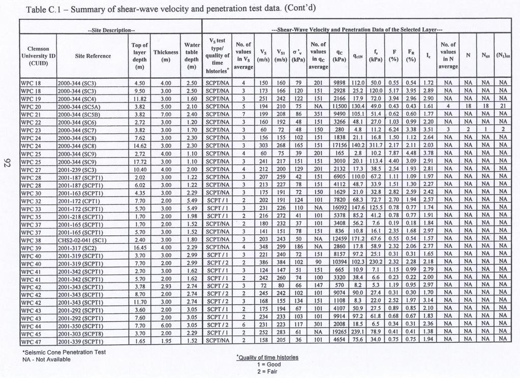
110

111

112

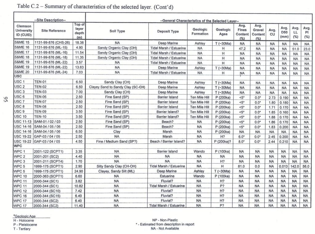
113

114

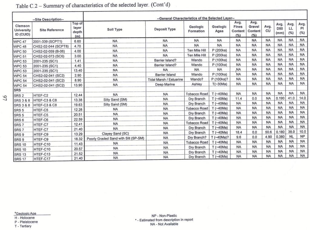
115