Regression with limited dependent variables. Professor Bernard Fingleton

Transcription

1 Regresson wth lmted dependent varables Professor Bernard Fngleton

2 Regresson wth lmted dependent varables Whether a mortgage applcaton s accepted or dened Decson to go on to hgher educaton Whether or not foregn ad s gven to a country Whether a job applcaton s successful Whether or not a person s unemployed Whether a company expands or contracts

3 Regresson wth lmted dependent varables In each case, the outcome s bnary We can treat the varable as a success (Y = 1) or falure (Y = 0) We are nterested n explanng the varaton across people, countres or companes etc n the probablty of success, p = prob( Y =1) Naturally we thnk of a regresson model n whch Y s the dependent varable

4 Regresson wth lmted dependent varables But the dependent varable Y and hence the errors are not what s assumed n normal regresson Contnuous range Constant varance (homoscedastc) Wth ndvdual data, the Y values are 1(success) and 0(falure) the observed data for N ndvduals are dscrete values 0,1,1,0,1,0, etc not a contnuum The varance s not constant (heteroscedastc)

5 Bernoull dstrbuton probablty of a success ( Y = 1) s p probablty of falure ( Y = 0) s 1- p = q EY ( ) = p var( Y) = p(1 p) as p vares for = 1,...,N ndvduals then both mean and varance vary EY ( ) = p var( Y ) = p (1 p ) regresson explans varaton n EY ( ) = p as a functon of some explanatory varables EY ( ) = f( X,..., X ) 1 K but the varance s not constant as EY ( ) changes whereas n OLS regresson, we assume only the mean vares as X vares, and the varance remans constant

6 The lnear probablty model ths s a lnear regresson model Y = b + b X +... b X + e K K Pr( Y = 1 X,..., X ) = b + b X +... b X b 1 1 K K K s the change n the probablty that Y = 1 assocated wth a unt change n X, holdng constant X.... X, etc Ths can be estmated by OLS but 1 2 Note that snce var( Y ) s not constant, we need to allow for heteroscedastcty n tf, tests and confdence ntervals K

7 The lnear probablty model 1996 Presdental Electon 3,110 US Countes bnary Y wth 0=Dole, 1=Clnton

8 The lnear probablty model Ordnary Least-squares Estmates R-squared = Rbar-squared = sgma^2 = Durbn-Watson = Nobs, Nvars = 3110, 2 *************************************************************** Varable Coeffcent t-statstc t-probablty Constant prop-gradprof prop-gradprof = pop wth grad/professonal degrees as a proporton of educated (at least hgh school educaton)

9 The lnear probablty model 1.5 Clnton Dole prop-gradprof = pop wth grad/professonal degrees as a proporton of educated (at least hgh school educaton)

10 The lnear probablty model Dole_Clnton_1 versus prop_gradprof (wth least squares ft) 1 Y = X 0.8 Dole_Clnton_ prop_gradprof

11 The lnear probablty model Lmtatons The predcted probablty exceeds 1 as X becomes large Y ˆ = X f X > then Yˆ > 1 X = 0 gves Yˆ = f X < 0 possble, then X < gves Yˆ < 0

12 Solvng the problem We adopt a nonlnear specfcaton that forces the dependent proporton to always le wthn the range 0 to 1 We use cumulatve probablty functons (cdfs) because they produce probabltes n the 0 1 range Probt Uses the standard normal cdf Logt Uses the logstc cdf

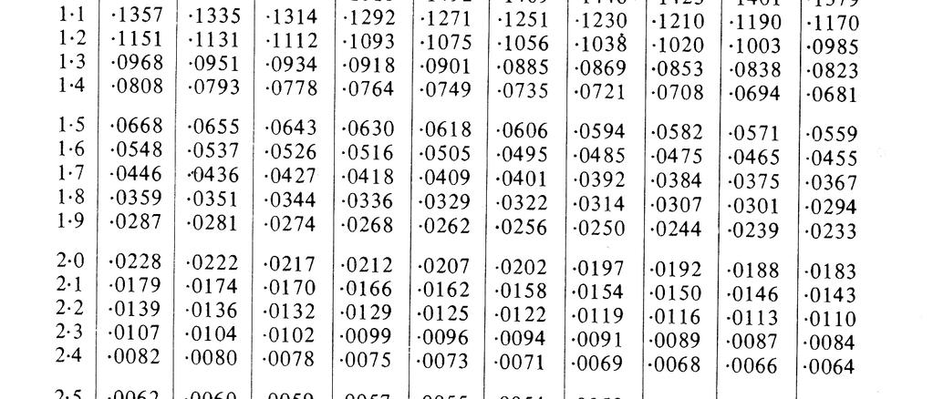
13 Probt regresson Φ ( z) = area to left of z n standard normal dstrbuton Φ ( 1.96) = Φ (0) = 0.5 Φ (1) = 0.84 Φ (3.0) = we can put any value for z from - to +, and the outcome s 0 < p = Φ ( z) < 1

14

15 Probt regresson Pr( Y = 1 X, X ) =Φ ( b + b X + b X ) eg b = 1.6, b = 2, b = 0.5 X = 0.4, X = 1 z = b + b X + b X = x x1 = Pr( Y = 1 X, X ) =Φ( 0.3) =

16 Probt regresson Model 9: Probt estmates usng the 3110 observatons Dependent varable: Dole_Clnton_1 VARIABLE COEFFICIENT STDERROR T STAT SLOPE (at mean) const prop_gradprof log_urban prop_hghs

17 Probt regresson Actual and ftted Dole_Clnton_1 versus prop_gradprof 1 ftted actual 0.8 Dole_Clnton_ prop_gradprof

18 Probt regresson Interpretaton The slope of the lne s not constant As the proporton of graduate professonals goes from 0.1 to 0.3, the probablty of Y=1 (Clnton) goes from 0.5 to 0.9 As the proporton of graduate professonals goes from 0.3 to 0.5 the probablty of Y=1 (Clnton) goes from 0.9 to 0.99

19 Probt regresson Estmaton The method s maxmum lkelhood (ML) The lkelhood s the jont probablty gven specfc parameter values Maxmum lkelhood estmates are those parameter values that maxmse the probablty of drawng the data that are actually observed

20 Probt regresson Pr( Y = 1) condtonal on X,..., X s p =Φ ( b + b X +... b X ) 1 K K K Pr( Y = 0) condtonal on X,..., X s 1- p = 1 Φ ( b + b X +... b X ) 1 K K K y s the value of Y observed for ndvdual for 'th ndvdual, Pr( Y y = y ) s p (1 p ) y for = 1,.., n, jont lkelhood s L=Π Pr( Y = y ) =Π p (1 p ) y [ ] [ ] L= Π Pr( Y = y ) =Π Φ ( b + b X +... b X ) 1 Φ ( b + b X +... b X ) log lkelhood s = { Φ + + } + (1 y )ln { 1 Φ ( b + b X +... b X } 1 y K K K K K K K K ln L yln ( b b X... b X 0 1 we obtan the values of b, b,..., b that gve the maxmum value of ln L K 1 y 1 y

21 Hypothetcal bnary data success X

22 Iteraton 0: log lkelhood = Iteraton 1: log lkelhood = Iteraton 2: log lkelhood = Iteraton 3: log lkelhood = Iteraton 4: log lkelhood = Iteraton 5: log lkelhood = Iteraton 6: log lkelhood = Iteraton 7: log lkelhood = Convergence acheved after 8 teratons Model 3: Probt estmates usng the 24 observatons 1-24 Dependent varable: success VARIABLE COEFFICIENT STDERROR T STAT SLOPE (at mean) const X

23 Model 3: Probt estmates usng the 24 observatons 1-24 Dependent varable: success VARIABLE COEFFICIENT STDERROR T STAT SLOPE (at mean) const X If X = 6, probt = Φ ( *6) =Φ ( ) = 0.45

24 Actual and ftted success versus X 1 ftted actual success X

25 Logt regresson Based on logstc cdf Ths looks very much lke the cdf for the normal dstrbuton Smlar results The use of the logt s often a matter of convenence, t was easer to calculate before the advent of fast computers

26 Logstc functon f(z) EPRO z logt

27 Z e z 1 Prob success = = 1+ e Z 1+ e Z Z Z e 1+ e e 1 Prob fal = 1- = = = Z Z Z Z 1+ e 1+ e 1+ e 1+ e Z Z Prob success e 1+ e Z odds rato = = = e Z Prob fal 1+ e 1 log odds rato = z e z 1 z = b0+ b1x1+ b2x bkx k

28 Logstc functon p = b + b X 0 1 p plotted aganst X s a straght lne wth p <0 and >1 possble p p = exp( b0 + b1x) 1 + exp( b + b X) 0 1 plotted aganst X gves s-shaped logstc curve so p > 1 and p < 0 mpossble equvalently p ln = b0 + b X 1 1 p ths s the equaton of a straght lne, so p ln plotted aganst X s lnear 1 p

29 Estmaton - logt X s fxed data, so we choose b, b, hence p p exp( b0 + b1x) = 1 + exp( b + b X) so that the lkelhood s maxmzed

30 Logt regresson z = b + b X +... b X K K Pr( Y = 1) condtonal on X,..., X s p = [1 + exp( z)] 1 K Pr( Y = 0) condtonal on X,..., X s 1- p = 1 [1 + exp( z)] 1 K y s the value of Y observed for ndvdual for 'th ndvdual, y Pr( Y = y ) s p (1 p ) y for = 1,.., n, jont lkelhood s L=Π Pr( Y = y ) =Π p (1 p ) 1 y 1 1 y 1 L= Π Pr( Y = y) =Π [1 + exp( z)] 1 [1 + exp( z)] log lkelhood s 1 ln L= yln {[1 + exp( z)] } + (1 y)ln{ 1 [1 + exp( ( z)] 1 } we obtan the values of b, b,..., b that gve the maxmum value of ln L K 1 y 1 y

31 Estmaton maxmum lkelhood estmates of the parameters usng an teratve algorthm

32 Estmaton Iteraton 0: log lkelhood = Iteraton 1: log lkelhood = Iteraton 2: log lkelhood = Iteraton 3: log lkelhood = Iteraton 4: log lkelhood = Iteraton 5: log lkelhood = Iteraton 6: log lkelhood = Convergence acheved after 7 teratons Model 1: Logt estmates usng the 24 observatons 1-24 Dependent varable: success VARIABLE COEFFICIENT STDERROR T STAT SLOPE (at mean) const X

33 VARIABLE COEFFICIENT STDERROR T STAT SLOPE (at mean) const X If X = 6, logt = *6 = = ln(p/(1-p) P = exp( )/{1+exp( )} = 1/(1+exp(0.5654)) =

34 Actual and ftted success versus X 1 ftted actual success X

35 Modellng proportons and percentages

36 The lnear probablty model consder the followng ndvdual data for Y and Y = 0,0,1,0,0,1,0,1,1,1 X = 1,1, 2, 2,3,3, 4, 4,5,5 constant = 1,1,1,1,1,1,1,1,1,1 X Yˆ = X s the OLS estmate Notce that the X values for ndvduals 1 and 2 are dentcal, lkewse 3 and 4 and so on If we group the dentcal data, we have a set of proportons p = 0/2, 1/2, 1/2, 1/2, 1 = 0, 0.5, 0.5, 0.5, 1 X = 1,2,3,4,5 pˆ = X s the OLS estmate

37 The lnear probablty model When n ndvduals are dentcal n terms of the varables explanng ther success/falure Then we can group them together and explan the proporton of successes n n trals Ths data format s often mportant wth say developng country data, where we know the proporton, or % of the populaton n each country wth some attrbute, such as the % of the populaton wth no schoolng And we wsh to explan the cross country varatons n the %s by varables such as GDP per capta or nvestment n educaton, etc

38 Regresson wth lmted dependent varables Wth ndvdual data, the values are 1(success) and 0(falure) and p s the probablty that Y = 1 the observed data for N ndvduals are dscrete values 0,1,1,0,1,0, etc not a contnuum Wth grouped ndvduals the proporton p s equal to the number of successes Y n n trals (ndvduals) So the range of Y s from 0 to n The possble Y values are dscrete, 0,1,2,,n, and confned to the range 0 to n. The proportons p are confned to the range 0 to 1

39 Modellng proportons Proporton (Y/n( Y/n) ) Contnuous response 5/10 = /3 = /9 = /10 = /20 = /2 =

40 Bnomal dstrbuton the moments of the number of successes n trals, each ndependent, = 1,..., N p s the probablty of a success n each tral EY ( ) = np var( Y ) = n p (1 p ) the varance s not constant, but depends on Y ~ B( n, p ) Y n and p

41 Data Regon Cleveland,Durham Cumbra Northhumberland Humbersde N Yorks Output growth survey of startup frms q starts(n) expanded(y) propn =Y/n

42 The lnear probablty model Regresson Plot Y = X R-Sq = 48.9 % 1.0 propn =e/s gvagr

43 OLS regresson wth proportons y = x Predctor Coef StDev T P Constant x S = R-Sq = 48.9% R-Sq(adj) = 47.3% Negatve proporton Proporton > 1 Ftted values = y = x

44 Grouped Data Regon Cleveland,Durham Cumbra Northhumberland Humbersde N Yorks Output growth survey of startup frms q starts(n) expanded(y) propn =Y/n

45 Proportons and counts ln( p / (1 p ) = b + b X 0 1 ln( pˆ / (1 pˆ ) = bˆ + bˆ X EY ( ) Yˆ = = n pˆ np 0 1 n Yˆ = sze of sample = estmated expected number of successes n sample

46 Bnomal dstrbuton For regon n! Pr ob( Y = y) = p (1 p) y!( n y)! y n y n = number of ndvduals p = probablty of a success Y = number of successes n n ndvduals

47 Bnomal dstrbuton For regon n! Pr ob( Y = y) = p (1 p) y!( n y)! Example P =0.5, n = 10 ob Y 10! = = = 5!(10 5)! y n y 5 5 Pr ( 5) 0.5 (0.5) EY ( ) = np= 5 var( Y) = np(1 p) = 2.5

48 Y s B(10,0.5) E(Y)=np = 5 var(y)=np(1-p)= Frequency C25 Y s B(10,0.9) E(Y)=np = 9 var(y)=np(1-p)= Frequency C27

49 Maxmum Lkelhood proportons Assume the data observed are Y = y = 5 successes from 10 trals and Y = y = 9 successes from 10 trals what s the lkelhood of these data gven p = 0.5, p = 0.9? n! Pr ob( Y = 5) = p (1 p ) 1 y n y y1!( n1 y1)! ! 5 5 Pr ob( Y1 = 5) = 0.5 (0.5) = !(10 5)! n! Pr ob( Y = 9) = p (1 p ) Y 2 y n y y2!( n2 y2)! ! = = = 9!(10 9)! 9 1 Pr ob( 2 9) 0.9 (0.1) lkelhood of observng y = 5, y = 9 gven p = 0.5, p = 0.9 = x = However lkelhood of observng y = 5, y = 9 gven p = 0.1, p = 0.8 = x =

50 Inference

51 Lkelhood rato/devance Y = 2ln( L / L )~ χ 2 2 u r L u = lkelhood of unrestrcted model wth k1 df L r = lkelhood of restrcted model wth k2 df k2 > k1 Restrctons placed on k2-k1 k1 parameters typcally they are set to zero

52 Devance Ho: b = 0, = 1,...,( k2 k1) 2 = 2ln( / )~ 2 u r k2 k1 Y L L χ 2 E( Y ) = k2 k1

53 Iteraton 7: log lkelhood = Convergence acheved after 8 teratons = Lu Model 3: Probt estmates usng the 24 observatons 1-24 Dependent varable: success VARIABLE COEFFICIENT STDERROR T STAT SLOPE (at mean) const X Model 4: Probt estmates usng the 24 observatons 1-24 Dependent varable: success VARIABLE COEFFICIENT STDERROR T STAT SLOPE (at mean) const Log-lkelhood = Comparson of Model 3 and Model 4: Null hypothess: the regresson parameters are zero for the varables X =Lr 2{Lu Lr]= 2[ ] = Test statstc: Ch-square(1) = , wth p-value = e-006 Of the 3 model selecton statstcs, 0 have mproved. Nb 2ln(Lu/Lr) = 2* ( ) =

54 Iteraton 3: log lkelhood = Convergence acheved after 4 teratons Model 2: Logt estmates usng the 3110 observatons Dependent varable: Dole_Clnton_1 VARIABLE COEFFICIENT STDERROR T STAT SLOPE (at mean) const log_urban prop_hghs prop_gradprof Model 3: Logt estmates usng the 3110 observatons Dependent varable: Dole_Clnton_1 VARIABLE COEFFICIENT STDERROR T STAT SLOPE (at mean) const prop_hghs Log-lkelhood = Comparson of Model 2 and Model 3: Null hypothess: the regresson parameters are zero for the varables log_urban prop_gradprof Test statstc: Ch-square(2) = , wth p-value = e-016

55 DATA LAYOUT FOR LOGISTIC REGRESSION REGION URBAN SE/NOT SE OUTPUT GROWTH Y n Hants, IoW suburban SE Kent suburban SE Avon suburban not SE Cornwall, Devon rural not SE Dorset, Somerset rural not SE S Yorks urban not SE W Yorks urban not SE

56 Logstc Regresson Table Predctor Coef StDev Z P Constant gvagr URBAN/SUBURBAN/RURAL suburban urban SOUTH-EAST/NOT SOUTH-EAST South-East Log-Lkelhood =

57 Testng varables Prob = f(q) Log-lke degrees of freedom Prob = f(q,urban,se) *Dfference = > 7.81, the crtcal value equal to the upper 5% pont of the ch-squared dstrbuton wth 3 degree of freedom thus ntroducng URBAN/SUBURBAN/RURAL and SE/not SE causes a sgnfcant mprovement n ft

58 Interpretaton When the transformaton gves a lnear equaton lnkng the dependent varable and the ndependent varables then we can nterpret t n the normal way The regresson coeffcent s the change n the dependent varable per unt change n the ndependent varable, controllng for the effect of the other varables For a dummy varable or factor wth levels, the regresson coeffcent s the change n the dependent varable assocated wth a shft from the baselne level of the factor

59 Interpretaton ln( Pˆ /(1 Pˆ ) Changes by for a unt change n gvagr by as we move from not SE to SE countes by as we move from RURAL to URBAN by as we move from RURAL to SUBURBAN

60 Interpretaton The odds of an event = rato of Prob(event) to Prob(not event) The odds rato s the rato of two odds. The logt lnk functon means that parameter estmates are the exponental of the odds rato (equal to the logt dfferences).

61 Interpretaton For example, a coeffcent of zero would ndcate that movng from a non SE to a SE locaton produces no change n the logt Snce exp(0) = 1, ths would mean the (estmated) odds = Prob(expand)/Prob(not expand) do not change e the odds rato =1 In realty, snce exp(2.441) = the odds rato s The odds of SE frms expandng are tmes the odds of non SE frms expandng

62 Interpretaton param. est. s.e. t rato p-value odds rato lower c.. upper c.. Constant gvagr E+05 RURAL/SUBURBAN/URBAN suburban urban SE/not SE SE Note that the odds rato has a 95% confdence nterval snce * = and * * = and exp(3.1338)=22.96, exp(1.7484) = 5.75 The 95% c..for the odds rato s 5.75 to 22.96