Direct Sum. McKelvey, and Madie Wilkin Adviser: Dr. Andrew Christlieb Co-advisers: Eric Wolf and Justin Droba. July 23, Michigan St.

Transcription

1 and Adviser: Dr. Andrew Christlieb Co-advisers: Eric Wolf and Justin Droba Michigan St. University July 23, 2014

2 The N-Body Problem Solar systems

3 The N-Body Problem Solar systems Interacting charges, gases and plasma

4 The N-Body Problem Solar systems Interacting charges, gases and plasma We want to solve the system of ODE s given by: dx i dt = v i dv i dt = a i = F i(x 1,..., x n ) m i for i = 1,..., n.

5 Traditional Solutions Particle Mesh Particle-Particle Particle-Mesh

6 The net force on particle i is: F i = n q i E j,i j=1 j i

7 The net force on particle i is: F i = n q i E j,i j=1 j i E j,i is the electric field from particle j at the location of particle i and q i is the charge

8 The net force on particle i is: F i = n q i E j,i j=1 j i E j,i is the electric field from particle j at the location of particle i and q i is the charge To calculate the force on all of the particles, we must repeat this summation for each of the n particles

9 The net force on particle i is: F i = n q i E j,i j=1 j i E j,i is the electric field from particle j at the location of particle i and q i is the charge To calculate the force on all of the particles, we must repeat this summation for each of the n particles The problem with direct sum is that it is O(N 2 )

10 Goal Find efficient ways to solve the n-body problem.

11 Goal Find efficient ways to solve the n-body problem. Improve efficiency from O(n 2 ) to O(n) + O(k 2 ) where k << n and k is the number of particles per cell. Table: Theoretical Time Comparison (3600 MHz computer) E j,i = q j ɛ 0 G(x j x i ) F j,i = q i E j,i N O(N 2 ) O(N) sec 10 9 sec sec 10 7 sec min 10 4 sec yrs.28 sec yrs 4.6 min

12 We are working on it. We made a Finite Difference Mesh based method, which is a variation of the Particle-Particle Particle-Mesh method, that improved efficiency from O(n 2 ) to approximately O(n)

13 We are working on it. We made a Finite Difference Mesh based method, which is a variation of the Particle-Particle Particle-Mesh method, that improved efficiency from O(n 2 ) to approximately O(n) We want to compute the field on the particles quickly

14 We are working on it. We made a Finite Difference Mesh based method, which is a variation of the Particle-Particle Particle-Mesh method, that improved efficiency from O(n 2 ) to approximately O(n) We want to compute the field on the particles quickly

15 x (n) i, v (n 1/2) i Interpolate ρ (n) x (n+1) i Leapfrog v (n 1/2) i Poisson Solve Leapfrog φ (n) Finite E (n) Interpolate a (n) Difference i

16 x (n) i, v (n 1/2) i Interpolate ρ (n) x (n+1) i Leapfrog v (n 1/2) i Poisson Solve Leapfrog φ (n) Boundary E (n) Interpolate Integral a (n) i Corrected

17 Using Finite Difference to Solve ( x, ȳ + h) ( x h, ȳ) ( x + h, ȳ) ( x, ȳ h) Five-Point Stencil ( x, ȳ + h) ( x h, ȳ + h) ( x + h, ȳ + h) ( x h, ȳ) ( x + h, ȳ) ( x h, ȳ h) ( x, ȳ h) ( x + h, ȳ h) Nine-Point Stencil

18 Using Finite Difference to Solve ( x, ȳ + h) ( x h, ȳ) ( x + h, ȳ) ( x, ȳ h) Five-Point Stencil 2 φ = xx φ + yy φ ( x, ȳ + h) ( x h, ȳ + h) ( x + h, ȳ + h) ( x h, ȳ) ( x + h, ȳ) ( x h, ȳ h) ( x, ȳ h) ( x + h, ȳ h) Nine-Point Stencil

19 Using Finite Difference to Solve ( x h, ȳ) ( x, ȳ + h) ( x, ȳ h) ( x + h, ȳ) ( x, ȳ + h) ( x h, ȳ + h) ( x + h, ȳ + h) ( x h, ȳ) ( x + h, ȳ) ( x h, ȳ h) ( x, ȳ h) ( x + h, ȳ h) Five-Point Stencil Nine-Point Stencil 2 φ = xx φ + yy φ 2 φ = φ j+1,k 2φ j,k +φ j 1,k + φj,k+1 2φ j,k +φ j,k 1 + O( x 2 + y 2 ) ( x) 2 ( y) 2 where j is the index for x and k is the index for y

20 Using Finite Difference to Solve ( x h, ȳ) ( x, ȳ + h) ( x, ȳ h) ( x + h, ȳ) Five-Point Stencil 2 φ = xx φ + yy φ 2 φ = φ j+1,k 2φ j,k +φ j 1,k ( x) 2 ( x, ȳ + h) ( x h, ȳ + h) ( x + h, ȳ + h) ( x h, ȳ) ( x + h, ȳ) ( x h, ȳ h) ( x, ȳ h) ( x + h, ȳ h) Nine-Point Stencil + φj,k+1 2φ j,k +φ j,k 1 ( y) 2 + O( x 2 + y 2 ) where j is the index for x and k is the index for y A φ = ρ

21 Using Finite Difference to Solve ( x h, ȳ) ( x, ȳ + h) ( x, ȳ h) ( x + h, ȳ) Five-Point Stencil 2 φ = xx φ + yy φ 2 φ = φ j+1,k 2φ j,k +φ j 1,k ( x) 2 ( x, ȳ + h) ( x h, ȳ + h) ( x + h, ȳ + h) ( x h, ȳ) ( x + h, ȳ) ( x h, ȳ h) ( x, ȳ h) ( x + h, ȳ h) Nine-Point Stencil + φj,k+1 2φ j,k +φ j,k 1 ( y) 2 + O( x 2 + y 2 ) where j is the index for x and k is the index for y A φ = ρ E y (x, y) = φ(x,y+h) φ(x,y h) 2h, E x (x, y) = φ(x+h,y) φ(x h,y) 2h

22 Acceleration is used to find the velocity at t = n +.5

23 Acceleration is used to find the velocity at t = n +.5 That velocity is then used to find the position of each particle at t = n + 1

24 Acceleration is used to find the velocity at t = n +.5 That velocity is then used to find the position of each particle at t = n + 1 This is the leapfrog algorithm

25 Acceleration is used to find the velocity at t = n +.5 That velocity is then used to find the position of each particle at t = n + 1 This is the leapfrog algorithm v 1/2 = v 0 + a 0 dt 2 v n+1/2 = v n 1/2 + a n dt x n = x n 1 + v n 1/2 dt

26 Deriving Green s Identity φ(x) = N i=1 G(x i x 0 ) (G(x x 0 ) φ φ G(x x 0 )) nds V

27 Deriving Green s Identity φ(x) = N i=1 G(x i x 0 ) (G(x x 0 ) φ φ G(x x 0 )) nds V V F dv = V F nds

28 Deriving Green s Identity φ(x) = N i=1 G(x i x 0 ) (G(x x 0 ) φ φ G(x x 0 )) nds V V F dv = V F nds Let F = θγ where θ is a scalar function, γ = ψ is a vector function. ( θ 2 ψ + θ ψ ) dv = (θ ψ n) ds V V

29 Deriving Green s Identity φ(x) = N i=1 G(x i x 0 ) (G(x x 0 ) φ φ G(x x 0 )) nds V V F dv = V F nds Let F = θγ where θ is a scalar function, γ = ψ is a vector function. ( θ 2 ψ + θ ψ ) dv = (θ ψ n) ds V V If we let θ = G(x x 0 ) and ψ = φ, then we can solve for the potential φ(x)

30 We can use the fact that ρ = N δ(x x i ) i=1

31 We can use the fact that ρ = N δ(x x i ) i=1 We can solve for φ to obtain: φ(x) = N i=1 G(x i x 0 ) (G φ φ G) nds V

32 We can use the fact that ρ = N δ(x x i ) i=1 We can solve for φ to obtain: φ(x) = N i=1 G(x i x 0 ) (G φ φ G) nds V φ x,j = N i=1 i j 1 2π ln ( x i x j 2 ) + Ω (φ G G φ) n ds

33 We can use the fact that ρ = N δ(x x i ) i=1 We can solve for φ to obtain: φ(x) = N i=1 G(x i x 0 ) (G φ φ G) nds V φ x,j = N i=1 i j 1 2π ln ( x i x j 2 ) + Ω (φ G G φ) n ds New equation because Potential Theory tells us it is the same φ x,j = N i=1 i j 1 2π ln ( x i x j 2 ) + Ω σ s(y)g (x j y) ds(y)

34 We can use the fact that ρ = N δ(x x i ) i=1 We can solve for φ to obtain: φ(x) = N i=1 G(x i x 0 ) (G φ φ G) nds V φ x,j = N i=1 i j 1 2π ln ( x i x j 2 ) + Ω (φ G G φ) n ds New equation because Potential Theory tells us it is the same φ x,j = N i=1 i j 1 2π ln ( x i x j 2 ) + Ω σ s(y)g (x j y) ds(y) σ is like a surface charge

35 We use direct sum to calculate the field due to local particles

36 We use direct sum to calculate the field due to local particles In order to evaluate the boundary integral, we solve using numerical quadrature.

37 We use direct sum to calculate the field due to local particles In order to evaluate the boundary integral, we solve using numerical quadrature. We end up with a matrix that we have to invert to obtain the surface charge.

38 We use direct sum to calculate the field due to local particles In order to evaluate the boundary integral, we solve using numerical quadrature. We end up with a matrix that we have to invert to obtain the surface charge. Then, instead of doing this everywhere which would be O(n 2 ), we make this a subcell method which gives O(n) + O(k 2 ).

39 Solving for Sigma s2 s 1 σg ds

40 Solving for Sigma s2 s 1 σg ds We take a limit to the boundary with respect to variable x and get the integral equation

41 Solving for Sigma s2 s 1 σg ds We take a limit to the boundary with respect to variable x and get the integral equation We turn the integral into discrete approximations that we can solve

42 Solving for Sigma s2 s 1 σg ds We take a limit to the boundary with respect to variable x and get the integral equation We turn the integral into discrete approximations that we can solve The integral becomes four sums

43 Solving for Sigma s2 s 1 σg ds We take a limit to the boundary with respect to variable x and get the integral equation We turn the integral into discrete approximations that we can solve The integral becomes four sums We use integral mean value theorem and trapezoid rule to end up with the Green s matrix 4k i=1 s2 s 1 σg ds

44 Solving for Sigma s2 s 1 σg ds We take a limit to the boundary with respect to variable x and get the integral equation We turn the integral into discrete approximations that we can solve The integral becomes four sums We use integral mean value theorem and trapezoid rule to end up with the Green s matrix 4k i=1 s2 s 1 σg ds Then we end up with a system of equations in which we need to perform a Green s matrix inversion

45 In order to get the Boundary Integral Corrected Electric Fields we need several things

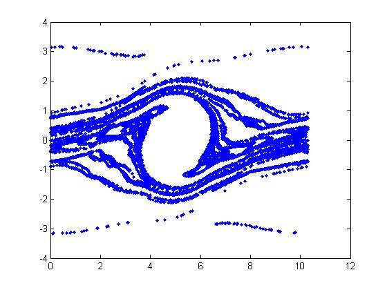
46 In order to get the Boundary Integral Corrected Electric Fields we need several things List of all particles inside the cell

47 List of all particles in boundary cells

48 Potential at all 12 border points per cell

49 Something to take the above and calculate the electric field

50 For loop over all cells

51 For loop over all cells If we can get this done, then it s a matter of increasing customizability

52

53 Figure: Uncorrected

54 Figure: Point charge at the center