CIMPA research school Non-commutative algebra. The center and the Lie structure of a Leavitt path algebra Mercedes Siles Molina

Transcription

1 CIMPA research school Non-commutative algebra The center and the Lie structure of a Leavitt path algebra Mercedes Siles Molina From 19 to 28 October 2015 Penonomé, Coclé

2

3 Contents Contents i Abstract 1 1 Preliminary results Leavitt path algebras The grading Cycles Ordering paths Ideals Hereditary and saturated sets of vertices The ideal generated by line points The ideal generated by vertices in cycles without exits The ideal generated by extreme cycles The center of a Leavitt path algebra The extended centroid The center Simplicity of related Lie algebras 47 References 49 i

4 ii

5 1 Abstract These notes contain all the explanations and references corresponding to the course I delivered during the first CIMPA research school in Panama in October 2015 (see the complete program of the school here: up.ac.pa/program.html). The purpose of the course is to explain the essentials on Leavitt path algebras and then to determine the center of a Leavitt path algebra whose associated graph is row finite. We start by the very beginning of the theory of Leavitt path algebras and give the tools needed to understand the structure of the center. Finally, we give a taste of the work that has been done concerning the study of the Lie estructure of a Leavitt path algebra. Panama, October 2015.

6 2

7 Chapter 1 Preliminary results We introduce the main object of this course: Leavitt path algebras. A directed graph is a 4-tuple E = (E 0, E 1, r E, s E ) consisting of two disjoint sets E 0, E 1 and two maps r E, s E : E 1 E 0. The elements of E 0 are called the vertices of E and the elements of E 1 the edges of E while for e E 1, r E (e) and s E (e) are called the range and the source of e, respectively. If there is no confusion with respect to the graph we are considering, we simply write r(e) and s(e). 3

8 4 Chapter 1. Preliminary results Given a (directed) graph E and a field K, the path K-algebra of E, denoted by KE, is defined as the free associative K-algebra generated by the set of paths of E with relations: (V) vw = δ v,w v for all v, w E 0. (E1) s(e)e = er(e) = e for all e E 1. If s 1 (v) is a finite set for every v E 0, then the graph is called row-finite. If E 0 is finite and E is row-finite, then E 1 must necessarily be finite as well; in this case we say simply that E is finite. A vertex which emits no edges is called a sink. A vertex v is called an infinite emitter if s 1 (v) is an infinite set, and a regular vertex otherwise. The set of infinite emitters will be denoted by Einf 0 while Reg(E) will denote the set of regular vertices. The extended graph of E is defined as the new graph Ê = (E0, E 1 (E 1 ), rê, sê), where (E 1 ) = {e i e i E 1 } and the functions rê and sê are defined as rê E 1 = r, s Ê E 1 = s, r Ê (e i ) = s(e i ), and sê(e i ) = r(e i ). The elements of E 1 will be called real edges, while for e E 1 we will call e a ghost edge.

9 1.1. Leavitt path algebras Leavitt path algebras. The Leavitt path algebra of E with coefficients in K, denoted L K (E), is the quotient of the path algebra KÊ by the ideal of KÊ generated by the relations: (CK1) e e = δ e,e r(e) for all e, e E 1. (CK2) v = {e E 1 s(e)=v} ee for every v Reg(E).

10 6 Chapter 1. Preliminary results

11 1.1. Leavitt path algebras. 7 Condition (CK2) can be seen in the following example. Observe that in KÊ the relations (V) and (E1) remain valid and that the following is also satisfied: (E2) r(e)e = e s(e) = e for all e E 1. Note that if E is a finite graph, then L K (E) is unital with v E 0 v = 1 LK (E); otherwise, L K (E) is a ring with a set of local units consisting of sums of distinct vertices (for a ring R the assertion R has local units means that each finite subset of R is contained in a corner of R, that is, a subring of the form ere where e is an idempotent of R). Note that since every Leavitt path algebra L K (E) has local units, it is the directed union of its corners. A path µ in a graph E is a finite sequence of edges µ = e 1... e n such that r(e i ) = s(e i+1 ) for i = 1,..., n 1. In this case, s(µ) := s(e 1 ) and r(µ) := r(e n ) are the source and range of µ, respectively, and n is the length of µ. We also say that µ is a path from s(e 1 ) to r(e n ) and denote by µ 0 the set of its vertices, i.e., µ 0 := {s(e 1 ), r(e 1 ),..., r(e n )}. By µ 1 we denote the set of edges appearing in µ, i.e., µ 1 := {e 1,..., e n }. We view the elements of E 0 as paths of length 0. The set of all paths of a graph E is denoted by Path(E).

12 8 Chapter 1. Preliminary results There are many examples of known algebras that can be seen as Leavitt path algebras. Here we see some. 1.2 The grading. The Leavitt path algebra L K (E) is a Z-graded K-algebra, spanned as a K- vector space by {αβ α, β Path(E)}. In particular, for each n Z, the degree n component L K (E) n is spanned by the set {αβ α, β Path(E) and length(α) length(β) = n}. is, Denote by h(l K (E)) the set of all homogeneous elements in L K (E), that h(l K (E)) := n Z L K (E) n. 1.3 Cycles. If µ is a path in E, and if v = s(µ) = r(µ), then µ is called a closed path based at v. If s(µ) = r(µ) and s(e i ) s(e j ) for every i j, then µ

13 1.3. Cycles. 9 is called a cycle. A graph which contains no cycles is called acyclic. For µ = e 1... e n Path(E) we write µ for the element e n... e 1 of L K (E). An edge e is an exit for a path µ = e 1... e n if there exists i {1,..., n} such that s(e) = s(e i ) and e e i. We say that E satisfies Condition (L) if every cycle in E has an exit. Let X be a subset of E 0. A path in X is a path α in E with α 0 X. We say that a path α in X has an exit in X if there exists e E 1 which is an exit for α and such that r(e) X.

14 10 Chapter 1. Preliminary results We denote by P c (E) (P c if there is no confusion about the graph) the set of vertices of a graph E lying in cycles without exits, and decompose it as: P c (E) = P c (E) + P c (E), where P c (E) + are those elements in P c (E) for which there exists a cycle without exits c such that the number of paths ending at a vertex of c 0 and not containing all the edges of c is infinite, P c (E) = P c (E) \ P c (E) + and denotes the disjoint union. If it is clear from the context the graph we are referring to, we will write simply P c + or Pc. 1.4 Ordering paths. Given paths α, β, we say α β if β = αα for some path α.

15 Chapter 2 Ideals In this chapter we will speak mainly about graded ideals of Leavitt path algebras. Of course, in an arbitrary Leavitt path algebra not every ideal has to be graded. This is the case, for example, of the Leavitt path algebra associated to the graph E having one vertex, say v, and one edge, say e. It is isomorphic to the Laurent polynomial ring K[x, x 1 ] and here not every ideal is graded. For example, < 1 + x > is not a graded ideal. This, translated to L K (E) means that < v + e > is not a graded ideal. Before stating some results on graded ideals, we will recall here the characterization of simple Leavitt path algebras (those algebras A whose unique ideals are 0 and A). Recall that for a graph E, the set H E consists of all hereditary and saturated subsets of vertices of E. Also, we recall that a graph E is said to satisfy Condition (L) if every cycle has an exit. Theorem 2.1. (The Simplicity Theorem) Let E be an arbitrary graph and K any field. Then the Leavitt path algebra L K (E) is simple if and only if E satisfies the following conditions: (i) H E = {, E 0 }. (ii) E satisfies Condition (L) 2.1 Hereditary and saturated sets of vertices We define a relation on E 0 by setting v w if there exists a path in E from v to w. A subset H of E 0 is called hereditary if v w and v H imply w H. A hereditary set is saturated if every regular vertex which feeds into H and only into H is again in H, that is, if s 1 (v) is finite and 11

16 12 Chapter 2. Ideals r(s 1 (v)) H imply v H. Denote by H E the set of hereditary saturated subsets of E 0. Hereditary and saturated subsets of vertices play an important role in the theory of Leavitt path algebras. In fact, they are closely related to graded ideals of Leavitt path algebras (as was highlighted for the first time in [10]), and also to general ideals since every ideal I in a Leavitt path algebra L K (E) contains a graded part: the ideal generated by I E 0 (see [2, Theorem 2.8.6]). Let X be a subset of vertices in E 0. Denote by I(X) the ideal of L K (E) generated by X. Then, I(X) is a graded ideal. The reason is that it is generated by elements of degree zero. Moreover, if E is a row-finite graph every graded ideal J of L K (E) is I(H) for H a hereditary and saturated subset of E 0 ; concretely, H = J E 0 (see [16, Lemma 2.1 and Remark 2.2]). Although not every hereditary subset has to be saturated, hereditary subsets (much more easy to get) give important information about the Leavitt path algebra. Whenever X is a set of vertices of a graph E, the saturated closure of X is defined as i N Λ i (X), where Λ 0 (X) = X and by recurrence Λ i (X) = Λ i 1 (X) {v Reg(E) r(s 1 (v)) Λ i 1 (X)}. In particular, for a hereditary subset of vertices, say H, this saturated closure is hereditary and saturated and is denoted by H. For X a subset of vertices in a graph E, the hereditary closure of X is defined as the minimum hereditary subset of E 0 containing X. It always exists because is just the intersection of all hereditary subsets of E 0 which contains X. The hereditary and saturated closure of a set of vertices is defined as the saturated closure of the hereditary closure. Lema 2.2. Let E be a graph and K a field. Let H be a hereditary subset of E 0. Then { n } I(H) = k i γ i λ i n 1, k i K, γ i, λ i Path(E), r(γ i ) = r(λ i ) H. i=1 Moreover, if H denotes the saturated closure of H, then I(H) = I(H). Proof. Let I be the set in the second part of the identity in the statement. To see that I is an ideal of L K (E) we show that for every element αβ, where r(α) = r(β) = u H, and for every a, b L K (E), we have aαuβ b J. It is enough to prove that γλ uµη I for every γ, λ, µ, η Path(E) and u H. If γλ uµη = 0 we are done. Suppose otherwise that γλ uµη 0.Then γλ uµη = γµ η if µ = λµ, or γλ uµη = γ(λ ) η if λ = µλ. Note that u = s(µ) and H hereditary imply r(µ) H, therefore, r(µ ) = r(µ) H

17 2.1. Hereditary and saturated sets of vertices 13 in the first case, and r(λ ) = r(µ) H in the second case, which imply γλ uµη J in both cases. This shows that J is an ideal of L K (E); as it contains H and must be contained in every ideal containing H, it must coincide with I(H). Now we prove I(H) = I(H). Clearly I(H) I(H). The converse can be proved by induction (see [2, Lemma 2.4.1]). Results that will be very useful are the following. Lema 2.3. Let E be an arbitrary graph and let H 1, H 2 be non empty hereditary subsets of vertices of E. Then: (i) Λ m (H i ) is hereditary for every m N. (ii) H 1 H 2 = H 1 H 2. Proof. (i). For m = 0 the result is trivial. Suppose the result true for m 1 and let us show it for m. Take u Λ m (H i ) and let e E 1 be such that s(e) = u. Then r(e) r(s 1 (u)) Λ m 1 (H i ) Λ m (H i ). This implies the result. (ii). It is immediate to see H 1 H 2 H 1 H 2. For the converse we will prove: Λ m (H 1 ) Λ m (H 2 ) = Λ m (H 1 H 2 ). Note that the first observation implies Λ m (H 1 ) Λ m (H 2 ) Λ m (H 1 H 2 ). For the converse containment, use induction. If m = 0 then the result is trivially true. Suppose our assertion is true for m 1 and show it for m. If u Λ m (H 1 ) Λ m (H 2 ) then u Λ m 1 (H 1 ) or r(s 1 (u)) Λ m 1 (H 1 ). In the first case, and since Λ m 1 (H 1 ) is hereditary (by (i)) we have also r(s 1 (u)) Λ m 1 (H 1 ). Analogously we prove r(s 1 (u)) Λ m 1 (H 2 ). This means r(s 1 (u)) Λ m 1 (H 1 ) Λ m 1 (H 2 ) = Λ m 1 (H 1 H 2 ) (by the induction hypothesis) and so u Λ m (H 1 H 2 ). Lema 2.4. Let E be a graph and H a hereditary subset of E 0. Then, for every v H there exists a finite number of paths α 1,..., α n satisfying r(α i ) H and v = n i=1 α iα i. Proof. For v in H we get immediately the result. Take v in Λ 1 (H) not being a sink. Then v = f s 1 (v) ff and we have the claim. Suppose the result true for every u Λ i 1 (H) and take v Λ i (H). Then, for every f s 1 (v), since r(f) r(s 1 )(v) Λ i 1 (H), by the induction hypothesis, there exists a finite number of paths β f 1,..., βm f in Path(E) such that r(f) = i βf i (βf i ) and r(β f i ) H. Hence v = f s 1 (v) ff = f f( i βf i (βf i ) )f = f,i fβf i (βf i ) f and we have finished.

18 14 Chapter 2. Ideals The result that follows was stated for the first time in [14, Proposition 3.1] (although in that paper the statement is slightly different); it has proved to be very useful in many different contexts, for example in order to get the Uniqueness Theorems (see [14, Theorem 3.5]), to prove that every Leavitt path algebra is semisimple, etc. In this notes we also find another context where it can be used. Except otherwise stated, E will denote an arbitrary graph and K an arbitrary field. As usual, we will use the notation K for K \ {0}. Theorem 2.5. (The Reduction Theorem.) For every nonzero element a in a Leavitt path algebra L K (E), there exist α, β Path(E) such that: (i) 0 α aβ = kv for some k K and v E 0, or (ii) 0 α aβ = p(c, c ), where c is a cycle without exits in E and p(c, c ) denotes the evaluation of a polynomial p(x, x 1 ) K[x, x 1 ] at c. Of special interest will be the following result. Corollary 2.6. Let a be a nonzero homogeneous element in a Leavitt path algebra L K (E). Then, there exist α, β Path(E), k K and v E 0, such that 0 α aβ = kv. Proof. Let α, β Path(E) be such that 0 α aβ is as in cases (i) or (ii) in Theorem 2.5. In the first case, we have finished. In the second one, use the grading to obtain that in fact p(c, c ) in (ii) has to be a monomial, that is, α aβ = kc m for some k K and a certain integer m. If m = 0, there is nothing more to do. If m > 0, then(c ) m α aβ = kr(c) and we are done. If m < 0, then α aβc m = kr(c) and the proof is complete. Another useful result which derives from Theorem 2.5 is: Corollary 2.7. Let H be a non-empty hereditary subset of a graph E. Then, for every nonzero homogeneous a I(H) there exist α, β Path(E) such that α aβ = kv for some k K and v H. Proof. Given the nonzero element a I(H) apply Corollary 2.6 and choose λ, µ Path(E) such that λ aµ = kw for some k K and w E 0. Observe that w I(H). Use Lemma 2.2 to write w = m i=1 k iλ i µ i with k i K, λ i, µ i Path(E), r(λ i ) = r(µ i ) H, and suppose λ i µ i λ j µ j for every i j. Then for v = r(µ 1 ), α = λµ 1 and β = µµ 1 we have α aβ = µ 1λ aµµ 1 = kµ 1wµ 1 = kµ 1µ 1 = kr(µ 1 ) = kv, which is nonzero and satisfies v H.

19 2.1. Hereditary and saturated sets of vertices 15 Proposition 2.8. Let {H i } i Λ be a family of hereditary subsets of a graph E such that H i H j = for every i j. Then: I ( i Λ H i ) = I ( i Λ H i ) = i Λ I(H i ) = i Λ I ( H i ). Proof. The union of any family of hereditary subsets is again hereditary, hence H := i ΛH i is a hereditary subset of E 0. By Lemma 2.2 every element a in I(H) can be written as a = n l=1 k lα l β l, where k l K, α l, β l Path(E) and r(α l ) = r(β l ) H. Separate the vertices appearing as ranges of the α l s depending on the H i s they belong to, and apply again Lemma 2.2. This gives a i ΛI(H i ) I(H) since H i H and so i ΛI(Hi ) = I(H). Now we prove that the sum of the I(H i ) s is direct. If this is not the case, since we are dealing with graded ideals, we may suppose that there exists a homogeneous element 0 a I(H j ) j i Λ I(H i) for some j Λ; by Corollary 2.7 there exist α, β Path(E) and k K such that 0 k 1 α aβ = w H j. Observe that w also belongs to I( j i Λ H i ). Write w = n l=1 k lα l βl, with k l K, α l, β l Path(E), r(α l ) = r(β l ) j i Λ H i, and assume that every summand is non-zero. Then 0 r(β 1 ) = β1β 1 = β1wβ 1 j i Λ H i. On the other hand, s(α 1 ) = w H j implies (since H j is a hereditary set) r(α 1 ) H j ; therefore, r(α 1 ) = r(β 1 ) H j ( j i Λ H i ), a contradiction. To conclude the proof we point out that the first and last identities follow from [16, Lemma 2.1]. A similar relation can be established for the ideal generated by the intersection of a family of hereditary subsets. Lema 2.9. Let {H i } i Λ be a family of hereditary subsets of an arbitrary graph E. Then: (i) I( i Λ H i ) = i Λ I(H i ). (ii) If Λ is finite, then I( i Λ H i ) = i Λ I(H i ). Proof. (i). By the isomorphism given in [2, Theorem ] among hereditary and saturated subsets of vertices and a special type of graded ideals, I( i Λ H i ) = i Λ I(H i ) = i Λ I(H i ). (ii). When Λ is finite, then i Λ H i = i Λ H i (use Lemma 2.3), and consequently I( i Λ H i ) = I( i Λ H i ) = i Λ I(H i ) = i Λ I(H i ).

20 16 Chapter 2. Ideals Before stating the result that will allow us to work with connected graphs, we need to recall that the ideal generated by a hereditary and saturated subset in a Leavitt path algebra is isomorphic to a Leavitt path algebra. Let E be a graph. For every non empty hereditary subset H of E 0, define F E (H) = {α = e 1... e n e i E 1, s(e 1 ) E 0 \H, r(e i ) E 0 \H for i < n, r(e n ) H}. Denote by F E (H) another copy of F E (H). For α F E (H), we write α to denote a copy of α in F E (H). Then, we define the graph as follows: 1. H E 0 = ( H E) 0 = H F E (H). HE = ( H E 0, H E 1, s, r ) 2. H E 1 = ( H E) 1 = {e E 1 s(e) H} F E (H). 3. For every e E 1 with s(e) H, s (e) = s(e) and r (e) = r(e). 4. For every α F E (H), s (α) = α and r (α) = r(α). The following result was first proved in [16, Lemma 5.2] and then in [11, Lemma 1.2] for row-finite graphs, although the result is valid in general (see [2, Theorem ]). Lema Let E be an arbitrary graph and K any field. For a hereditary subset H E 0, the ideal I(H) is isomorphic to the Leavitt path algebra L K ( H E). Concretely, there is an isomorphism (which is not graded) ϕ : L K ( H E) I(H) acting as follows: ϕ(v) = v for every v H, ϕ(α) = αα for every α F E (H), ϕ(e) = e and ϕ(e ) = e for every e E 1 such that s(e) H. ϕ(α) = α and ϕ(α ) = α for every α F E (H). When we build the Leavitt path algebra of a graph E, we consider paths not only in E, but in the extended graph Ê; this means that when we think of a connected graph we have in mind ghost paths too. For this reason we say that a graph E is connected if Ê is a connected graph in the usual sense, that is, if given any two vertices u, v E 0 there exist h 1,..., h m E 1 (E 1 )

21 2.1. Hereditary and saturated sets of vertices 17 such that η := h 1... h m is a path in KÊ (in particular it is non-zero) such that s(η) = u and r(η) = v. The connected components of a graph E are the graphs {E i } i Λ such that E is the disjoint union E = i Λ E i, where every E i is connected. Corollary Let E be a graph and suppose E = i Λ E i, where each E i is a connected component of E. Then L K (E) = i Λ L K (E i ). Proof. By Proposition 2.8, L K (E) = i Λ I(E 0 i ) and by Lemma 2.10, I(E 0 i ) is isomorphic to the Leavitt path algebra L K ( E 0 i E). Since the graph E 0 i E is just E i, the result follows. By means of this corollary, and for our purposes, from now on we will restrict our attention to Leavitt path algebras of connected graphs. Another application of Proposition 2.8 is stated below. Concretely, we will see that essentiality of graded ideals generated by hereditary and saturated subsets in a Leavitt path algebra (which is equivalent to density as one-sided ideals) can be expressed in terms of properties of the underlying graph. Proposition Let H be a hereditary subset of a graph E. Then I(H) is a dense (left/right) ideal if and only if every vertex of E 0 connects to a vertex in H. Proof. We first remark that since every Leavitt path algebra is left nonsingular (see [25, Proposition 4.1]), the notions of dense left/right ideal and that of essential are equivalent in this context (by [22, (8.7) Proposition]), and by [22, (14.1) Proposition], I(H) is essential as a left/right ideal if and only if it is essential as an ideal. Moreover, as I(H) is a graded ideal, by [23, Proposition] essentiality and graded essentiality of I(H) are equivalent. Hence, we will show that I(H) is a graded essential ideal if and only if every vertex of E 0 connects to a vertex in H. Suppose first that I(H) is a graded essential ideal of L K (E). Let v E 0. If H T (v) =, then Lemma 2.9 would imply I(H) I(T (v)) = 0, but this cannot happen as I(H) is a graded essential ideal. Hence H T (v). This implies that v connects to a vertex in H. Now we prove the converse, i.e., that I(H) is an essential graded ideal. Let J be a nonzero graded ideal and pick a nonzero homogeneous element x = uxv J, where u, v E 0. Since the Leavitt path algebra L K (E) is an algebra of right quotients of KE, by [24, Proposition 2.2] (which is valid even for non necessarily row-finite graphs) there exists µ Path(E) such that 0 xµ KE. Denote by w the range of µ. By the hypothesis w connects to a vertex in H, hence there exists λ Path(E) such that

22 18 Chapter 2. Ideals w = s(λ) and r(λ) H. If xµλ = 0 then xµ ul K (E)w KE would satisfy λ Path(E) ran(xµ) =, by [19, Lemma 1], a contradiction, hence 0 xµλ I(H) J which shows our claim. 2.2 The ideal generated by line points. There is a strong connection among properties of a Leavitt path algebra and properties of the graph. This is one of the advantages of considering these kind of algebras: you can visualize algebraic properties and can build algebras satisfying certain conditions. Here we show some of these connections. Let E be a graph. For v E 0, the tree of v, written T (v), denotes the set {w E 0 v w}. A vertex v E 0 is called a bifurcation vertex (or it is said that there is a bifurcation at v) if s 1 E (v) contains at least two edges of E. A vertex u E 0 is called a line point if there are neither bifurcations nor cycles at any vertex of T (u). Obviously, every sink is a line point. The set of line points of the graph E will be denoted by P l (E). It is always a hereditary subset of E 0 although it is not necessarily saturated.

23 2.3. The ideal generated by vertices in cycles without exits. 19 It is shown in [14, 15] that every line point generates a minimal left ideal, hence it is in the socle. It is not difficult to see (apply, for example [14, Propositon 2.6] that: Lema Let E be an arbitrary graph. Let v be a line point. Then: Moreover, vl K (E)v = K. Lema Let E be an arbitrary graph and let v be a line point. Then I(v) = M Λ (K), where Λ denotes a set whose cardinal coincides with the cardinal of all paths ending at v. It is possible to decompose P l (E) = H i, where every H i is a hereditary subset and I(H i ) = I(v i ) for some line point v i H i. Then, using Proposition 2.8 we get I(P l (E)) = i Λ M Λi (K). Moreover (see [2, Theorem ]): Theorem Let E be an arbitrary graph and K any field. Decompose P l (E) = i Γ H i as it has been explained. Then i Λ Soc(L K (E)) = I(P l (E)) = i Λ M Λi (K), where for every i Λ, if v i is an arbitrary element of H i then I(v i ) = M Λi (K). 2.3 The ideal generated by vertices in cycles without exits. A similar pattern as for line points can be applied to vertices in cycles without exits. The following result is [15, Lemma 1.5]. Lema Let E be an arbitrary graph. Let v be a vertex in E 0 such that there exists a cycle without exits c based at v. Then: { n } vl K (E)v = k i c i k i K; m, n N = K[x, x 1 ], i= m where = denotes a graded isomorphism of K-algebras, and considering (by abuse of notation) c 0 = w and c t = (c ) t, for any t 1.

24 20 Chapter 2. Ideals Proof. First, it is easy to see that if c = e 1... e n is a cycle without exits based at v and u T (v), then s(f) = s(g) = u, for f, g E 1, implies f = g. Moreover, if r(h) = r(j) = w T (v), with h, j E 1, and s(h), s(j) T (v) then h = j. We have also that if µ E and s(µ) = u T (v) then there exists k N, 1 k n verifying µ = e k µ and s(e k ) = u. Let x vl K (E)v be given by x = p i=1 k iα i βi +δv, with s(α i ) = r(βi ) = s(β i ) = v and α i, β i E. Consider A = {α E : s(α) = v}; we prove now that if α A, deg(α) = mn + q, m, q N with 0 q < n, then α = c m e 1... e q. We proceed by induction on deg(α). If deg(α) = 1 and s(α) = s(e 1 ) then α = e 1. Suppose now that the result holds for any β A with deg(β) sn + t and consider any α A, with deg(α) = sn + t + 1. We can write α = α f with α A, f E 1 and deg(α ) = sn + t, so by the induction hypothesis α = c s e 1... e t. Since s(f) = r(e t ) = s(e t+1 ) implies f = e t+1, then α = α f = c s e 1... e t+1. We shall show that the elements α i βi are in the desired form, i.e., c d with d Z. Indeed, if deg(α i ) = deg(β i ) and α i βi 0, we have α i βi = c p e 1... e k e k... e 1c p = v by (4). On the other hand deg(α i ) > deg(β i ) and α i βi 0 imply α i βi = c d+q e 1... e k e k... e 1c q = c d, d N. In a similar way, from deg(α i ) < deg(β i ) and α i βi 0 it follows that α i βi = c q e 1... e k e k... e 1c q d = c d, d N. Define ϕ: K[x, x 1 ] L K (E) by ϕ(1) = v, ϕ(x) = c and ϕ(x 1 ) = c. It is a straightforward routine to check that ϕ is a graded monomorphism with image vl K (E)v, so that vl K (E)v is graded isomorphic to K[x, x 1 ] as a graded K-algebra. The structure of the ideal generated by any vertex in a cycle without exists is known. See, for example [2, Lemma ]. Lema For any vertex v P c (E), let Λ v denote the (possibly infinite) set of paths in E which end at v, but which do not contain all the edges of c, where c is the cycle without exits such that s(c) = v. Then: I(c 0 ) = I(v) = M Λv (K[x, x 1 ]). Proof. It is easy to see that I(c 0 ) = I(v). To prove the isomorphism in the statement, consider the family B := {µc k η µ, η Λ v, k Z}, where as usual c 0 denotes v and c k denotes (c ) k for k < 0. Then B is a K-linearly independent set which generates I(v) (see [2, Lemma ]). The map ϕ : I(v) M Λv (K[x, x 1 ]) given by ϕ(µc k η ) = x k e µ,η

25 2.4. The ideal generated by extreme cycles. 21 where x k e µ,η denotes the element of M Λv (K[x, x 1 ]) which is x k in the (µ, η) entry, and zero otherwise is a K-algebra isomorphism. A consequence is the structure of the ideal generated by vertices in cycles without exits (see [2, Theorem 2.7.3]). Theorem Let E be an arbitrary graph and K any field. Then: I(P c (E)) = i Υ M Λi (K[x, x 1 ]), where {c i } i Υ is the set of different cycles without exits in E and Λ i is the set of paths in E which end at the base v i of the cycle c i, but do not contain all the edges of c i. The importance of the ideal I(P c (E)) relays also in that every ideal non containing vertices is contained in it (see [16] for a proof of this fact for row-finite graphs). 2.4 The ideal generated by extreme cycles. Now we introduce the notion of extreme cycle. Roughly speaking it is a cycle such that every path starting at a vertex of the cycle comes back to it. The ideal generated by extreme cycles will be proved to be a direct sum of purely infinite simple Leavitt path algebras. Definitions Let E be a graph and c a cycle in E. We say that c is an extreme cycle if c has exits and for every path λ starting at a vertex in c 0 there exists µ Path(E) such that 0 λµ and r(λµ) c 0. We will denote by P ec (E) the set of vertices which belong to extreme cycles. Definitions Let X ec be the set of all extreme cycles in a graph E. We define in X ec the following relation: given c, d X ec, we write c d whenever c and d are connected, that is, T (c 0 ) d 0, equivalently, T (d 0 ) c 0. It is not difficult to see that is an equivalence relation. Denote the set of all equivalence classes by X ec = X ec/. When we want to emphasize the graph we are considering we will write X ec(e) and X ec (E) for X ec and X ec, respectively. For any c X ec, let c denote the class of c and let use c 0 to represent the set of all vertices which are in the cycles belonging to c. The following will be of use. Remark For a graph E and using the notation described above:

26 22 Chapter 2. Ideals (i) For any c X ec, c 0 = T (c 0 ), hence c 0 is a hereditary subset. (ii) Given c, d X ec, c d if and only if c 0 d 0 =. (iii) For c, d X ec, c d if and only if T (c) = T (d). Examples Consider the following graphs E e f g F e h f g h 1 h 2 Then X ec(e) = {g, h}, X ec (E) = { g}, X ec(f ) = {e, fg, gf, h 1, h 2 } and X ec (F ) = {ẽ}. Now we will analyze the structure of the ideal generated by P ec (E). Lema Let E be an arbitrary graph and K any field. For every cycle c such that c X ec, the ideal I( c 0 ) is isomorphic to a purely infinite simple Leavitt path algebra. Concretely, to L K ( H E), where H = c 0. Proof. Use Lemma 2.10 to have I( c 0 ) isomorphic to the Leavitt path algebra L K ( H E) and let us show that this Leavitt path algebra is purely infinite and simple. For that, we will use the characterization [4, Theorem 4.3], which is valid for arbitrary graphs as can be proved by using the techniques described in [21] or in [12] in order to translate certain characterizations of Leavitt path algebras from the row-finite case to the case of an arbitrary Leavitt path algebra. Every vertex of H E connects to a cycle: take v H E 0 ; if v H then it connects to c, otherwise there exists a path µ Path(E) such that s(µ) = v and r(µ) H. Since r(µ) connects to the cycle c in E, the vertex v also connects to c in H E. Every cycle in H E has an exit: this follows because any cycle in this graph comes from a cycle d in H and, by construction, d = c; this means that d connects to c and hence it has an exit which is an exit in H E. The only hereditary and saturated subsets of H E 0 are and H E 0 : let H H H E be non empty and consider v H ; if v H then H H ; since H is saturated, H = H E 0 ; if v / H then there exists f H E 1 such that v = s(f) and r(f) H; this implies H H ; now, apply the construction of HE and that H is saturated to get H = H E 0.

27 2.4. The ideal generated by extreme cycles. 23 Proposition Let E be any graph and K any field. Then I(P ec (E)) = c Xec I( c 0 ) and every I( c 0 ) is isomorphic to a Leavitt path algebra which is purely infinite simple. Proof. The hereditary set P ec (E) can be decomposed as: P ec (E) = c Xec c 0. By the Remark 2.21 and the Proposition 2.8, I(P ec (E)) = I( c Xec c 0 ) = c Xec I( c 0 ). Finally, observe that every I( c 0 ) is isomorphic to a purely infinite simple Leavitt path algebra by Lemma Lema For any graph E the hereditary sets P l (E), P c (E) and P ec (E) are pairwise disjoint. Moreover, the ideal generated by their union is I(P l (E)) I(P c (E)) I(P ec (E)). Proof. By the definition of P l (E), P c (E) and P ec (E), they are pairwise disjoint. To get the result, apply Proposition 2.8. The following ideal, will be of use in order to establish the center of a Leavitt path algebra, so we name it here. Definition For a graph E we define I lce := I(P l (E)) I(P c (E)) I(P ec (E)). Theorem Let E be an arbitrary graph and K any field. Then: (i) I lce = ( i Λ1 M mi (K)) ( j Λ2 M nj (K[x, x 1 ]) ) ( l Λ3 I( c 0 n l ) ), where Λ 1 is the index set of the sinks of E, Λ 2 is the index set of the cycles without exits in E and Λ 3 indexes X ec (E). (ii) If E 0 < then I lce is a dense ideal of L K (E). Proof. For our purposes we may suppose that the graph E is connected because if E = i Λ E i is the decomposition of E into its connected components and we show the claims for every connected component, then the result will be true for E by virtue of Corollary (i). We know that I(P l (E)) is the socle of the Leavitt path algebra L K (E) (see [15, Theorem 5.2] and [8, Theorem 1.10]), moreover I(P l (E)) = i Λ1 M mi (K), where Λ 1 ranges over the sinks of E and for any i Λ 1, if s i is a sink (finite or not), then m i is the cardinal of the set of paths ending at s i. The structure of I(P c (E)) is also known: by [5, Proposition 3.5] (which also works for arbitrary graphs) I(P c (E)) = j Λ2 M nj (K[x, x 1 ]), where the cardinal of Λ 2 is the cardinal of the set of cycles without exits and n j is the

28 24 Chapter 2. Ideals cardinal of the set of paths ending at a given cycle without exits c j and not containing the edges appearing in the cycle. Finally, the structure of the third summand in I lce follows by Proposition (ii). Take a vertex v E 0. Since E 0 is finite then v connects to a line point, to a cycle without exists or to an extreme cycle. This means that every vertex of E connects to the hereditary set H := P l (E) P c (E) P ec (E). By Proposition 2.12 this means that I(H) is a dense ideal of L K (E) and by Lemma 2.25 it coincides with I lce. Remark Following a similar reasoning as in the proof of Theorem 2.27 it can be shown that any ideal of L K (E) generated by vertices in P is isomorphic to ( i Λ1 M mi (K)) ( j Λ2 M nj (K[x, x 1 ]) ) ( l Λ3 I( c 0 n l ) ) for some Λ 1, Λ 2, Λ 3. We specialize this result in the case of a prime Leavitt path algebra. Corollary Let E be a graph with a finite number of vertices such that L K (E) is a prime algebra. Then, we have the following three mutually exclusive cases: (i) There is a unique sink v in E and every vertex of E connects to v. In this case I(P l (E)) = I(T (v)) = M m (K), where m is the cardinal of the set of paths ending at v, or (ii) there is a unique cycle without exits c and every vertex of E connects to it. In this case I(P c (E)) = I(c 0 ) = M n (K[x, x 1 ]), where n is the cardinal of the number of paths ending at c and not containing all the edges of c, or (iii) X ec (E) = { c}, where c is an extreme cycle and every vertex of E connects to c. In this case I(P ec (E)) = I(c 0 ) is a purely infinite simple unital ring.

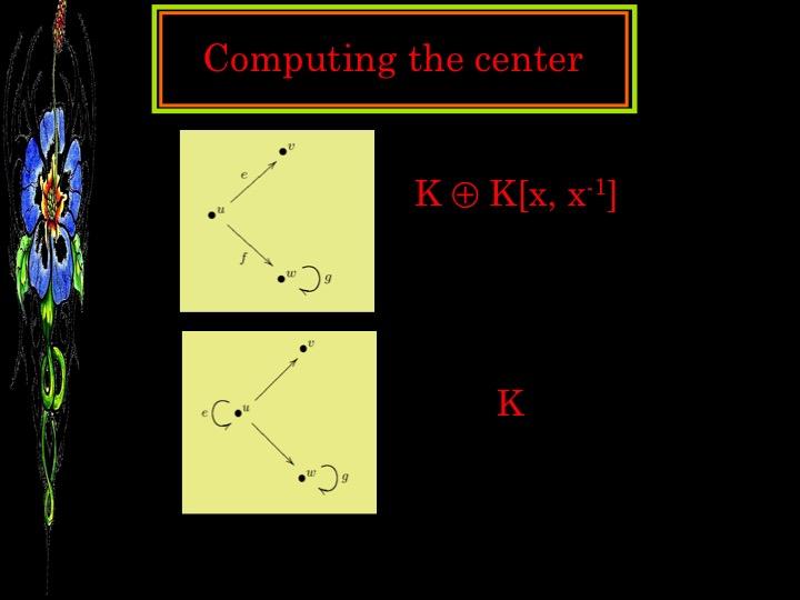
29 Chapter 3 The center of a Leavitt path algebra In this chapter we will completely describe the center of the Leavitt path algebra of a row-finite graph. Here are some of the reasons because of which we are interested in the center of a Leavitt path algebra. Relative to the simplicity of the Lie algebra related to an associative algebra, we have: 25

30 26 Chapter 3. The center of a Leavitt path algebra As for the general philosophy in Leavitt path algebras, we will see that the center can be computed by looking at the graph. That is, again, algebraic properties can be read from the graph. The key pieces for the description of the center are: the set of line points, the vertices in cycles without exits and the vertices in extreme cycles, jointly with an equivalence relation defined on E 0 whose set of classes is indexed in a subset of P := P l (E) P c (E) P ec (E). 3.1 The extended centroid of the Leavitt path algebra of a finite graph The extended centroid of the ideal generated by P will coincide with the center of the Martindale symmetric ring of quotients of the Leavitt path algebra, notion that plays an important role. Recall that for an associative algebra A, the center of A, denoted Z(A), is defined by: Z(A) := {x A [x, a] = 0 for every a A},

31 3.1. The extended centroid 27 where [a, b] := ab ba and juxtaposition stands for the product in the algebra A. For a semiprime algebra A, the extended centroid of A, denoted by C(A) is defined as: C(A) = Z(Q s (A)) = Z(Q l max(a)) = Z(Q r max(a)), where Q s (A), Q l max(a) and Q r max(a) are the Martindale symmetric ring of quotients of A, the maximal left ring of quotients of A and the maximal right ring of quotients of A, respectively (see [22, (14.18) Definition]). Lema 3.1. Let A be a unital simple algebra. Then Z(A) = C(A). Proof. We see first Z(A) C(A). Suppose this containment is not true. Then there exists x Z(A) and q Q s (A) such that xq qx 0. Use that Q s (A) is a right ring of quotients of A to find a A such that 0 (xq qx)a and qa A. Then 0 x(qa) q(xa) = (qa)x q(ax) = 0, a contradiction. To prove C(A) Z(A), consider q C(A) \ {0}. By [22, (14.22) Corollary], C(A) is a field, hence there exist q 1 C(A). Use again that Q s (A) is a right ring of quotients of A to find x A such that 0 q 1 x A. Since A is simple and unital Aq 1 xa = A, in particular there exists a finite number of elements a 1,..., a m, b 1,..., b m A such that 1 = m i=1 a iq 1 xb i. Multiply this identity by q and use that q is in the center of Q s (A) to get q = m i=1 a ixb i A as desired. Theorem 3.2. Let E be graph such that E 0 < and consider I := I lce. Then the extended centroid of L K (E) coincides with the extended centroid of I, C(I); moreover, C(L K (E)) = C(I) = ( m i=1k) ( n j=1k[x, x 1 ] ) ( ) n l=1k, where m is the number of sinks, n is the number of cycles without exits and n is the number of equivalence classes of extreme cycles. If P l (E), P c (E) or P ec (E) are empty, then the ideals they generate are zero and the corresponding summands in C(I) do not appear. Proof. As in the proof of Theorem 2.27 we may suppose that our graph is connected. Apply Theorem 2.27 (ii) and [22, (14.14) Theorem] to obtain Q s (L K (E)) = Q s (I). Then by [24, Lemma 1. 3 (i)] C(L K (E)) = C(I) = C (I(P l (E))) C (I(P c (E))) C (I(P ec (E))).

32 28 Chapter 3. The center of a Leavitt path algebra By Theorem 2.27 (i), Lemma 3.1 and Proposition 2.24, C(I(P ec (E))) = n l=1 C(I( c0 l )), where c l X ec and n = X ec. Use [13, Theorem 4.2] to obtain C(I( c 0 l )) = K for every l. To finish, use the three pieces of information in the paragraphs before to obtain C(L K (E)) = C(I) = ( m i=1k) ( n j=1k[x, x 1 ] ) ( n l=1 K) and we get the claim in the statement. 3.2 The center The following remarks and results will be useful to study the center of a Leavitt path algebra. Their proofs are straightforward. Remark 3.3. If A is an algebra and {I i } is a set of ideals of A whose sum is direct, then Z( i I i ) = i (Z(I i )). Lema 3.4. Let G be an abelian group. The center of a G-graded algebra A is G-graded, that is, if x Z(A) and x = g G x g is the decomposition of x into its homogenous components, then x g Z(A) for every g G. Proof. Indeed, for every y = h G y h in A, 0 = [x, y h ] = [ g G x g, y h ] = g G [x g, y h ]; using the grading on A and that G is abelian (to be sure that x g y h and y h x g are in the same homogeneous component) we get [x g, y h ] = 0 for any g G. Hence 0 = h G [x g, y h ] = [x g, g G y h] = [x g, y] which means x g Z(A). Notation 3.5. The homogeneous component of degree g in the center of a G-graded algebra A will be denoted by Z g (A). Lema 3.6. Let I be an ideal of an algebra A. If for every y Z(I) there exist n N and {a i, b i } n i=1 Z(I) such that y = n i=1 a ib i, then Z(I) = I Z(A). Proof. It is clear that I Z(A) Z(I). To show Z(I) Z(A), take y Z(I) and x A. Write y = n i=1 a ib i, for a i, b i Z(I). Then yx = n i=1 a ib i x = n i=1 a i(b i x) = n i=1 (b ix)a i = n i=1 b i(xa i ) = n i=1 (xa i)b i = xy. Corollary 3.7. Let I be an ideal of a Leavitt path algebra L K (E) such that for every y Z(I) there exist a, b Z(I) such that y = ab. Then Z(I) = I Z(L K (E)). This happens, in particular, for every ideal of L K (E) generated by vertices in P.

33 3.2. The center 29 Proof. The first statement follows immediately from Lemma 3.6 For I generated by vertices in P, by Remark 2.28, I is a direct sum of ideals of L K (E) which are isomorphic to M n (K), M n (K[x, x 1 ]) or J, for J purely infinite and simple. In this last case, by [19, Theorem 3.6], Z(J) is 0 or isomorphic to K; in the other cases, the centers are zero or isomorphic to K, or to K[x, x 1 ]. In all of these situations our hypothesis on the ideal is satisfied. Here are some previous papers related to the study of the center and of the derivations of a Leavitt path algebra. As for our contribution, we determine the center of some Cohn and graph path algebras, as well as the center of the Leavitt path algebra associated to a row finite graphs in these papers ([19, 20]):

34 30 Chapter 3. The center of a Leavitt path algebra The following definition was motivated by our analysis of the centers of different Leavitt path algebras. Here are some examples.

35 3.2. The center 31

36 32 Chapter 3. The center of a Leavitt path algebra

37 3.2. The center 33 Definitions 3.8. Let u, v E 0. The element λ u,v will denote a path such that s(λ u,v ) = u and r(λ u,v ) = v. In E 0 we define the following relation: given u, v E 0 we write u 1 v if and only if u = v or: (i) u v or v u and there are no bifurcations at any vertex in T (u) and T (v). (ii) there exist a cycle c, a vertex w c 0 and λ w,u,λ w,v P ath(e). This relation 1 is reflexive and symmetric. Consider the transitive closure of 1 ; we shall denote it by. The notation [v] will stand for the class of a vertex v. Example 3.9. The vertices u and v in the following graph are related: u v Remark The following is an example of a graph which illustrates why do we need to consider the transitive closure of the relation 1 in Definition 3.8. Note that u 1 v, v 1 w and u 1 w; however, u w. u v w In what follows we are going to describe the zero component of the center of a Leavitt path algebra L K (E) associated to a row-finite graph. Notation Let E be an arbitrary graph. Consider P = P l P c P ec and define X = P/. Decompose P = P f P, where P f are those elements v of P such that (i) [v] <, and (ii) F E ([v]) <

38 34 Chapter 3. The center of a Leavitt path algebra In the same vein we decompose X = X f X, where and X f = {[u] X forall v [u], v P f } X = {[u] X forsome v [u], v P }. Finally, we decompose X f = Xf l Xc f Xec f, where each of these subsets consists of equivalence classes induced by elements which are in P f P l, in P f P c and in P f P ec, respectively. Note that if u and v are vertices in P f, then u v if and only if u, v P l, u, v P c or u, v P ec. When we want to emphasize the graph E we are considering, we will write P l (E), X(E), etc. Lema Let E be an arbitrary graph and u, v P. Then: (i) [u] is a hereditary set. (ii) If u v then [u] [v] =. Proof. (i). Let w [u] and consider w r(s 1 (w)). Since w u there exists a finite set {v 1... v n } of vertices such that w = v 1 1 v v n = u. Note that w 1 v 2 and so w [u]. (ii). By the hypothesis [u] [v] =. Use (i) and Lemma 2.3 to get the result. Definition Let E be a graph and K be any field. An element a L K (E) which can be written as a = k [v] a [v], where k [v] K and a [v] = u + αα, [v] X f will be said to be written in the standard form. u [v] α F E ([v]) We will prove that every element in the zero component of the center of a Leavitt path algebra can be written in the standard form. Lema Let E be an arbitrary graph and K be any field. [v] X. For every u [v] and α, β F E ([v]) we have: Consider (i) If s(α) = s(β), then α β 0 if and only if α = β. (ii) If s(α) s(β) then α β = 0. (iii) uα = 0.

39 3.2. The center 35 Proof. (i). If α β 0 then α = βγ or β = αδ for some γ, δ Path(E). By the definition of F E ([v]), necessarily α = β. (ii). This case follows immediately. (iii). For u and α as in the statement, uα 0 implies u = s(α), but this is not possible as α F E ([v]). Notation For a graph E we denote by P e the set of vertices in cycles with exits. Lema Let E be an arbitrary graph. Then, for every a Z 0 and v P P e there exists k v K such that if u [v] then uau = k v u. Proof. Suppose first u = v. If v P c P e the result follows by [19, Corollary 7]. If v P l, by the proof of [8, Proposition 1.8] vl K (E)v = Kv, hence av = va Kv. Now, suppose u [v]. Since the relation is given as the transitive closure of 1, we may assume first that there exists a vertex w in a cycle, and paths λ, µ satisfying λ = wλu and µ = wµv. By the paragraph before there exists an element k K such that waw = kw. Then uau = ua = λ λa = λ aλ = λ (kw)λ = kλ λ = ku and analogously we show va = kv. Repeating this argument a finite number of steps we reach our claim. It is easy to see that when u is in the hereditary closure of [v] we also have the result. Finally, take u [v]. We may assume that u is not a sink (this case has been studied yet). By Lemma 3.12 (i) and Lemma 2.4 we may write u = n i=1 α iαi, where the α i s are paths and r(α i ) is in the hereditary closure of [v]. Then au = a n i=1 α iαi = n i=1 α iaαi = n i=1 α ikr(α i )αi = k n i=1 α iαi = ku. Proposition Let E be a row-finite graph and consider a nonzero homogeneous element a of degree zero in Z(L K (E)). Then: (i) av = 0 for every v P. (ii) a = [v] X f k [v] a [v] where a [v] = u [v] u + α F E ([v]) αα

40 36 Chapter 3. The center of a Leavitt path algebra Proof. (i). Suppose first [v] =. If av 0, by Lemma 3.16 we have au 0 for every u [v], which is an infinite set; this is not possible, so av = 0 and we have finished. Now, assume [v] <. Since v P, necessarily F E ([v]) =, then we have an infinite collection of paths {α n } n N F E ([v]) with α m α n for m n. Next we prove that as(α n ) 0 for each n. First, note that r(α n ) [v]; since av 0 then ar(α n ) 0 by Lemma 3.16, therefore 0 ar(α n ) = aα nα n = α nas(α n )α n which implies our claim. Since there is only a finite number of vertices u E 0 such that au 0, the set {s(α n )} n N must be finite. Moreover, the set [v], which contains all the ranges of the paths α n is finite. Since {α 0 n} n N < (because every vertex in α 0 n does not annihilate a by Lemma 3.16), v / P f and no vertex in α 0 n\r(α n ) is an infinite emitter, we may conclude that there is a path α m = γ 1... γ r... γ t, with γ i Path(E) such that l(γ r ) 1 and s(γ r ) = r(γ r ), hence α m contains a cycle based at s(γ r ), implying s(γ r ) [v]. This is a contradiction with the fact α m F E ([v]) and (i) has been proved. (ii). Write a = au, with u E 0 and au 0. If u v, with v P P e, then au = k v u by Lemma 3.16 and k v K. If u v for any v P P e then, as it is not a sink, by (CK2), we may write u = s(e)=u ee. Then au = a s(e)=u ee = s(e)=u eae. Take e in this summand. If r(e) P P e then ar(e) = k r(e) r(e) where k r(e) K and we get a summand as in the statement. Otherwise we apply (CK2) to r(e) and write r(e) = s(f)=r(e) ff ; then

41 3.2. The center 37 aee = ae s(f)=r(e) ff e. Every summand aeff e with r(f) P P e is k r(ef) eff e by Lemma 3.16, which is a summand as in the statement. For every nonzero summand not being in this case we apply again (CK2). This process stops because otherwise we would have an infinite path e 1 e 2... with e i E 0 such that s(e i ) s(e j ) for every i j and ae i 0 for every i, which is not possible as the number of vertices not annihilating a has to be finite. Note that the path e 1 e 2... e n we arrive at is, by construction, an element in F E ([v]). We remark that v P f by (i). Take v E 0 such that [v] X f and av 0; by Lemma 3.16 we have av = k v v for some k v K. Note that k v 0. For any u [v], Lemma 3.16 shows that au = k v u 0. If β F E ([v]), then by Lemma 3.14 β a = k r(β) β ββ. Since β a = aβ = ar(β)β = k v β, we get k r(β) = k v 0. This shows that a can be written as a linear combination of elements of the form where [v] X f. ( ) u + u [v] α F E ([v]) αα, Theorem Let E be a row-finite graph. For every class [v] X f, denote by a [v] = u [v] u + α F E ([v]) αα. Then B 0 = { a [v] [v] X f } is a basis of the zero component of the center of L K (E). Proof. By Proposition 3.17 every element in the zero component of the center is a linear combination of the elements of B 0. Lemmas 3.12 and 3.14 imply that B 0 is a set of linearly independent elements. In what follows we show that every a [v] in B 0 is in the center of L K (E). To start, consider a vertex w in E 0. It is not difficult to see wa [v] = a [v] w since a [v] is in n i=1u i L K (E)u i for a certain finite family of vertices {u i } n i=1. Consider and edge e in E and denote by A := [v] F E ([v]). We claim: ( ) r(e) A if and only if s(e) A or e A. Assume r(e) A. If s(e) / A then s(e) / [v] and since r(e) [v] we conclude that e F E ([v]) A. Reciprocally, if s(e) A then r(e) A because [v] is hereditary (Lemma 3.12 (i)). Finally, if e A then e F E ([v]) which implies r(e) A. Now we see that a [v] commutes with e. Suppose first that r(e) A. Then ea [v] = e by Lemma On the other hand, if s(e) A, then a [v] e = e + 0 = e by Lemma 3.14; if s(e) / A, then a [v] e = 0 + e = e by

42 38 Chapter 3. The center of a Leavitt path algebra Lemma Now, suppose r(e) / A. Then, by ( ) we have s(e), e / A. For each α we have eα = 0 or eα 0 and, in this last case, eα A since s(e) / A, by hypothesis, and r(e) = s(α) / A. Applying the results explained above, ea [v] = e αα = e αα + e eαα e. α F E ([v]) α F E ([v])α e=0 α F E ([v]) We claim that the second summand must be zero. Indeed, suppose e 2 α 0; then, s(e) w for a vertex w [v]; this implies s(e) [v], a contradiction since we assume s(e) / A. Therefore ea [v] = In what follows we compute a [v] e. a [v] e = = α F E ([v])α e=0 α F E ([v]) eαα = αα e + α F E ([v])α e=0 α F E ([v])α e=0 α F E ([v]) eαα + eαα (3.1) eαα e e = α F E ([v])α e 0 α F E ([v]) eαα. eαα e e (3.2) We claim that the second summand is zero. The reason is again that for α in the second summand, eα must be zero because α starts by e and α F E ([v]). Hence a [v] e = eαα = ea [v] by (3.1). α F E ([v])α e=0 Notation Let E be a graph. For a cycle c = e 1... e n in E and u i = s(e i ) we will write c ui to denote the cycle e i... e i 1. Let S be the set of all those cycles without exits c such that there is a finite number of paths ending at c and not containing c. Note that if c is a cycle in S and u, v c 0 with u v, then c u and c v will be different elements in S.

43 3.2. The center 39 Proposition Let E be an arbitrary graph and K any field. Consider a homogeneous element a in Z(L K (E)) with deg(a) > 0. Then au = 0 for all u P l P e. If u P c then au = k u c r u, where k u K, c u is a cycle without exits and r N. Moreover, if u P + c, then k u = 0. Proof. If u P l, then au = uau ul K (E)u = Ku, by [15, Proposition 4.7 and Remark 4.8], hence there exists λ K such that au = λu. Then λ must be zero as the degree of λu is zero and deg(a) > 0. Now, take u P e and let d be a cycle such that u = s(d). We will use partially a reasoning that appears in [19, Theorem 6]; we include it here for the sake of completeness. A generator system for ul K (E)u is A B, for and A = {d n (d m ) n, m 0} B = {d n αβ (d m ) n, m 0, α, β Path(E), s(α) = u = s(β), d α, β, α 1 β 1 d 1 }. For n = 0 we understand d n = u. Note that given n, m 0 and d n αβ (d m ) B, there exists a suitable r N such that (d r ) d n αβ (d m ) d r = 0. This gives us that if we define the map S : L K (E) L K (E) by S(x) = d xd, for every b B there is an n N satisfying S n (b) = 0. Note that au is a fixed point for S. A consequence of this reasoning is that au span(a). Write au = n k nd n (d m ), for m = n deg(a), where k n K. Then, for some l N we have au = S l (au) = n k nd deg(a). Since au commutes with every element in ul K (E)u, the same should happen to d deg(a), but this is not true as it does not commute with d, giving au = 0. Next we show the second part of the statement. For u P c, au = uau ul K (E)u = K[x, x 1 ] (by [12, Proposition 2.3]). Since deg(a) > 0, au = k u c r u for some r N\{0}, c u a cycle without exits and k u K. To finish, consider u P c + and write au = k u c r, for c a cycle without exits and k u K. Then, two cases can happen. First, assume that there exists a cycle d such that v := s(d) u and take a path α satisfying α = vαu. Then, as we have proved before, av = 0 and so k u c r = au = aα α = α aα = α avα = 0; this implies k u = 0 as required. In the second case there exists infinitely many paths γ n, for n N ending at v. Since E is row-finite (and

44 40 Chapter 3. The center of a Leavitt path algebra we are assuming that we are not in the first case, so there are no cycles involved), {s(γ n )} =. Then there exists m N such that as(γ m ) = 0 and so av = aγ mγ m = γ mas(γ m )γ m = 0 as desired. Lema Let E be a row-finite graph and K any field. For any homogeneous element a in Z(L K (E)) with deg(a) > 0 we have a = aαα, where α F E (c 0 ) for some cycle without exits c and r(α) P c. Proof. Let u be in E 0 such that au 0. Define T 1 (u) = {v T (u) e E 1, such that s(e) = u, r(e) = v}. Let T n (u) be ( ) T n (u) = {v T (u) \ T i(u) α Path(E), l(α) = n, i<n such that s(α) = u, r(α) = v}. Given 0 au, write au = a s 1 (u)=e ee = s 1 (u)=e eae (note that u cannot be a sink and so we may use (CK2)). By Proposition 3.20, the possibly nonzero summands are those eae such that r(e) T 1 (u) \ (P l P e P + c ). Let S 1 := {aee such that r(e) P c }. Now, to every element aee with r(e) T 1 (u) \ (P l P e P c ), apply Condition (CK2). Then aee = a(e s 1 (r(e))=f ff )e = (e s 1 (r(e))=f faf )e. Again by Proposition 3.20 the nonzero summands are those efaf e such that r(f) T 2 (u) \ (P l P e P + c ). Let S 2 := {aeff e such that r(f) P c }. This reasoning must stop in a finite number of steps, say m, because otherwise we would have infinitely many edges e 1, e 2... such that ae 1... e n 0 for every n. Since for every vertex w in a cycle aw = 0, the ranges of these paths are all different. Therefore, there would be infinitely many vertices not annihilating a, a contradiction. Note that, by construction, a = x m i=1 S i x and so a can be written as in the statement, where α F E (c 0 ) for some cycle without exits c. Lema Let E be an arbitrary graph and consider c u, d w F E (c 0 u), β F E (d 0 w) and n, m Z. S, α

45 3.2. The center 41 (i) If w = u, then α β 0 if and only if α = β. (ii) If w u then c m u α βd n w = 0. Proof. (i). If α β 0 then α = βγ or β = αδ for some γ, δ Path(E). In the first case, since r(β) c 0 u, by the very definition of F E (c 0 u) and taking into account α F E (c 0 u) we get α = β. In the second case we get analogously the same conclusion. The converse is obvious. (ii). Take w u and assume α β 0; this implies as before α = βγ or β = αδ for some γ, δ Path(E). In the first case, r(β) d 0 w; since d w has no exits, then γ 0 d 0 w. On the other hand, r(α) = r(γ) c 0 u d 0 w, therefore c 0 u = d 0 w and arguing as in (i) we conclude α = β. This implies c m u α βd n w = c m u d n w = 0 since w u. The other possibility yields the same conclusion. The following result will relate elements in the n component of the center to elements in the 0 component. Lema Let E an arbitrary graph and K any field. Let a be a nonzero element in Z(L K (E)). Then aa 0. Proof. By Theorem 2.5, there are α, β P ath(e) such that 0 α aβ = kv for some k K, v E 0, or 0 α aβ = p(c, c ), where p(c, c ) is a polynomial in a cycle without exits c. In the first case 0 k 2 v = (kv)(kv ) = α aββ a α = α ββ aa α, since a is in the center of L K (E), and so aa must be nonzero. In the second case, 0 p(c, c )p(c, c ) since p(c, c ) r(c)l K (E)r(c) which is isomorphic to the Laurent polinomial algebra K[x, x 1 ] (see [12, Proposition 2.3]), hence 0 α aββ a α = α ββ aa α, and so aa must be nonzero. Theorem Let E be a row-finite graph. Then, the set B n = m l(c)=n α F E (c 0 ) {c 0 } u c 0 is a basis of Z n (L K (E)) with n Z \ {0}. αc m u α c S Proof. We will assume n > 0. The case n < 0 follows by using the involution in the Leavitt path algebra.

46 42 Chapter 3. The center of a Leavitt path algebra Let a Z n (L K (E)). For every u E 0 such that au 0, Lemma 3.21 and Proposition 3.20 imply au = a αα = αar(α)α = αk α c mα α where α F E (c 0 ) {u}, r(α) P c and s(α) = u. Hence α = k α αc mα α α a = k α αc m v α, where the c v s are elements of S, α F E (c 0 ) {v} and r(α) P c. (3.3) Now we see that k α = k β for every α, β F E (c 0 ) appearing in the expresion before. We first note that αc r β is a nonzero element in L K (E) for every r N. Since aαβ = αβ a, using Lemma 3.22 we get k α αc m u β = k β αc m u β and so k α = k β. In what follows we prove that if c u appears in (3.3) then for every v c 0 u and for every β F E ([c 0 u]) we have that c v and βc v β also appear. Apply (3.3) and Lemmas 3.23 and 3.14 to get ( ) ( ) 0 aa = kα αc m v α kα αc m v α = kααvα 2. By Theorem 3.18, v must appears in this summand and also every β F E ([c 0 v]). This shows that the set B n generates the n-component of the center. In what follows we see that the elements of B n are linearly independent. In fact, we show that elements of the form αc m u α are linearly independent. To this end, let k α K and suppose k α αc mu u are different. Choose a nonzero βc mv v Lemma 3.22) β k β βc mv v been proved. β = k β c mv v α = 0, where all the summands β. Then 0 = β k α αc mu u α = (by β ; this implies k β = 0 and our claim has Finally we see that B n Z(L K (E)). Fix c u S and denote by A n = {αc m u α m.l(c u ) = n, α F E ([c 0 u]) {u}}, i.e., A n contains all the summands of a in (3.3). We see that for every β Path(E), A n β = βa n and A n β = β A n for all n Z; this will prove our statement. So, take αc m u α A n. Then αc m u α β is non zero if and only if β = α (by Lemma 3.22); in this case, αc m u α β = βc m u βa n. Suppose αc m u α β = 0; if βαc m u α = 0 then we have shown that 0 βa n ; otherwise βαc m u α 0; this implies r(β) = s(α). Now we distinguish two cases: first, α = u. Note that c m u β = 0 implies β c u γ, for any γ Path(E) and so βc m u β A n. Then

47 3.2. The center 43 0 = ββc m u β βa n (because r(β) = u). If α is not a vertex, then r(β) u hence 0 = βc m u βa n. This shows A n β βa n. For the converse, note that βαc m u α is nonzero if and only if βα is a nonzero element in F E ([c 0 u]), for w = s(β); in this case βαc m u α β A n and so βαc m u α = βαc m u α β β A n β. Now, suppose βαc m u α = 0. Then, multiplying on the right hand side by α(c m u ) and on the left hand side by β we get r(β)α = 0. If c m u β = 0 we have shown 0 = c m u β A n β. If c m u β 0, as c u has no exits, then β = c s uλ, where λ is such that c u starts by λ. If l(c u ) = 1, then β = c s u for some s N; we see that this implies αc m u α β = 0. Suppose otherwise αc m u α β 0. Then α β 0 and so α β or β α. The first case is not possible (note that neither c 1 u α 1 nor α = u), hence β α, implying s(α) = u. This happens only when α = u, but this is not possible as 0 = βαc m u α = cu s+m is a contradiction. Now, suppose l(c) > 1. Let e be the last edge in c u. Then ec m u e β, which is an element in A n β, is zero (because the first edge of β is the first one of c u, which is not e). This proves βa n A n β and therefore A n β = βa n. Applying the involution we have β A n = A n β for all n Z, as required. Definitions Let E be an arbitrary graph. Denote by P b the set of all vertices in E such that T (v) has infinite bifurcations. Define H f := [v] and H := [v] P b. [v] X f [v] X Proposition Let E be a row-finite graph and K be any field. Then L K (E) = I(H f ) I(H ). Proof. We will show v I(H f H ) for every v E 0. If v H f H we have finished. Suppose that this is not the case. In particular, this means s 1 (v). Write v = e s 1 (v) ee. If for every e in this sum r(e) H f H, then we have finished. If for some e, r(e) is a sink, we have finished; if r(e) is a vertex in a cycle, taking into account that every vertex of E 0 connects to H f H then r(e) u for some u H f H. Note that u / P b as otherwise v P b, and we are assuming v / H f H, therefore r(e) w X [w]. For those e s 1 (v) in the remaining cases we apply again Condition (CK2) to u 1 := r(e) and write u 1 = f s 1 (u 1 ) ff. Now we proceed in the same way concerning r(f). This process must stop because otherwise there would be infinitely many bifurcations and so v P b, a contradiction. Apply Proposition 2.8 to the disjoint hereditary subsets H f H to get the result.

48 44 Chapter 3. The center of a Leavitt path algebra Theorem (Structure Theorem for the center of a row-finite graph). Let E be a row-finite graph. Then: More concretely, Z(L K (E)) = K X\Xc f K[x, x 1 ] Xc f Z(L K (E)) = K Xl f K Xec f K[x, x 1 ] Xc f. Proof. By Proposition ( 3.26, ) L K (E) = I(H f ) I(H ). Since H f := [v] Xf [v] and H := [v] X [v] P b, Proposition 2.8 implies hence L K (E) = I([v]) I(H ), [v] X f Z(L K (E)) = Z(I([v]) Z(I(H )). [v] X f By Theorems 3.18 and 3.24 we know Z(L K (E)) [v] X f Z(I([v])); therefore