pyoptfem Documentation

Transcription

1 pyoptfem Documentation Release V0.0.6 F. Cuvelier November 09, 2013

2

3 CONTENTS 1 Presentation Classical assembly algorithm (base version) Sparse matrix requirement Optimized classical assembly algorithm (OptV1 version) New Optimized assembly algorithm (OptV2 version) D benchmarks Benchmark usage Mass Matrix Stiffness Matrix Elastic Stiffness Matrix D benchmarks Benchmark usage Mass Matrix Stiffness Matrix Elastic Stiffness Matrix FEM2D module Assembly matrices (base, OptV1 and OptV2 versions) Element matrices (used by base and OptV1 versions) Vectorized tools (used by OptV2 version) Vectorized element matrices (used by OptV2 version) Mesh FEM3D module Assembly matrix (base, OptV1 and OptV2 versions) Element matrix (used by base and OptV1 versions) Vectorized tools (used by OptV2 version) Vectorized element matrix (used by OptV2 version) Mesh valid2d module Mass Matrix Stiffness matrix Elastic Stiffness Matrix valid3d module Mass Matrix Stiffness matrix Elastic Stiffness Matrix i

4 8 Quick testing 95 9 Testing and Working Requirements Installation License issues Indices and tables 105 Python Module Index 107 Index 109 ii

5 pyoptfem is a Python module which aims at measuring and comparing the performance of three programming techniques for assembling finite element matrices in 2D and 3D. For each of the matrices studied, three assembly versions are available: base, OptV1 and OptV2 Three matrices are currently implemented (more details are given in FEM2D module and FEM3D module) : Mass matrix : M i,j = φ j (q) φ i (q)dq, (i, j) {1,..., n q } 2. Ω h Stiffness matrix : S i,j = φ j (q). φ i (q)dq, (i, j) {1,..., n q } 2. Ω h Elastic stiffness matrix : K m,l = ε t (ψ l (q))σ(ψ m (q))dq, (m, l) {1,..., dn q } 2. Ω h Contents: where d is the space dimension. CONTENTS 1

6 2 CONTENTS

7 CHAPTER ONE PRESENTATION Let Ω h be a triangular (2d) or tetrahedral (3d) mesh of Ω R d corresponding to the following data structure: name type dimension description n q integer 1 number of vertices n me integer 1 number of elements q double d n q array of vertices coordinates. q(ν, j) is the ν-th coordinate of the j-th vertex, ν {1,..., d}, j {1,..., n q }. The j-th vertex will be also denoted by q j me integer (d + 1) n me connectivity array. me(β, k) is the storage index of the β-th vertex of the k-th element, in the array q, for β {1,..., (d + 1)} and k {1,..., n me } volumes double 1 n me array of volumes in 3d or areas in 2d. volumes(k) is the k-th element volume (3d) or element area (2d), k {1,..., n me } Scalar finite elements : Let H 1 h (Ω h) = {v C 0 (Ω h ), v T P 1 (T ), T T h }, be the finite dimensional space spanned by the P 1 -Lagrange (scalar) basis functions {φ i } i {1,...,nq} where P 1 (T ) denotes the space of all polynomials defined over T of total degree less than or equal to 1. The functions φ i satisfy φ i (q j ) = δ i,j, (i, j) {1,..., n q } 2 Then we have φ i 0 on T k, k {1,..., n me } such that q i / T k. A P 1 -Lagrange (scalar) finite element matrix is of the generic form D i,j = D(φ j, φ i )dω h, (i, j) {1,..., n q } 2 Ω h where D is the bilinear differential operator (order 1) defined for all u, v H 1 h (Ω h) by D(u, v) = A u, v (u b, v v u, c ) + duv and A (L (Ω h )) d d, b (L (Ω h )) d, c (L (Ω h )) d and d L (Ω h ) are given functions on Ω h. We can notice that D is a sparse matrix due to support properties of φ i functions. Let n dfe = d + 1. The element matrix D α,β (T k ), associated to D, is the n dfe n dfe matrix defined by D α,β (T k ) = D(φ k β, φ k α)(q)dq, (α, β) {1,..., n dfe } 2 T k 3

8 where φ k α = φ me(α,k) is the α-th local basis function associated to the k-th element. For examples, the Mass matrix is defined by M i,j = φ j φ i dω h Ω h The corresponding bilinear differential operator D is completely defined with A = 0, b = c = 0 and d = 1. the Stiffness matrix is defined by S i,j = φ j, φ i dω h Ω h The corresponding bilinear differential operator D is completely defined with A = I, b = c = 0 and d = 0. Vector finite elements : The dimension of the space (H 1 h (Ω h)) d is n df = d n q. in dimension d = 2, we have two natural basis : the global alternate basis B a defined by { ( φ1 B a = {ψ 1,..., ψ 2nq } = 0 ), ( 0, φ1) ( ) ( ( ) ( ) } φ2 0 φnq 0,,...,, 0 φ2) 0 φ nq and the global block basis B b defined by B b = {φ 1,..., φ 2nq } = { ( ) ( ) ( ) ( ( ( ) } φ1 φ2 φnq 0 0 0,,...,,,,..., φ1) φ2) φ nq in dimension d = 3, we have two natural basis : the global alternate basis B a defined by φ B a = {ψ 1,..., ψ 3nq } = 0, φ 1, 0,..., 0 0 φ 1 φ nq , φ nq, 0 0 φ nq and the global block basis B b defined by φ 1 B b = {φ 1,..., φ 3nq } = 0,..., 0 φ nq , φ 1,..., φ nq, 0,..., φ 1 φ nq 4 Chapter 1. Presentation

9 A P 1 -Lagrange (vector) finite element matrix in B a basis is of the generic form H l,m = H(ψ m, ψ l )dω h, (l, m) {1,..., dn q } 2 Ω h where H is the bilinear differential operator (order 1) defined by d H(u, v) = D α,β (u α, v β ) α,β=1 and D α,β is a bilinear differential operator of scalar type. For example, in dimension d = 2, the Elastic Stiffness matrix is defined by K m,l = ε t (ψ l (q))cε(ψ m (q)), (m, l) {1,..., 2n q } 2. Ω h where ε = (ε xx, ε yy, ε xy ) t is the strain tensor respectively and C is the Hooke matrix λ + 2μ λ 0 C = λ λ + 2μ μ Then the bilinear differential operator associated to this matrix is given by ( ) ( ) λ + 2μ 0 0 μ H(u, v) = 0 μ u 1, v 1 + λ 0 u 2, v 1 ( ) ( ) 0 λ μ 0 + μ 0 u 1, v λ + 2μ u 2, v 2 We present now three algorithms (base, OptV1 and OptV2 versions) for assembling this kind of matrix. Note: These algorithms can be successfully implemented in various interpreted languages under some assumptions. For all versions, it must have a sparse matrix implementation. For OptV1 and OptV2 versions, we also need a particular sparse matrix constructor (see Sparse matrix requirement). And, finally, OptV2 also required that the interpreted languages support classical vectorization operations. Here is the current list of interpreted languages for which we have successfully implemented these three algorithms : Python with Numpy and Scipy modules, Matlab, Octave, Scilab 5

10 1.1 Classical assembly algorithm (base version) Due to support properties of P 1 -Lagrange basis functions, we have the classical algorithm : Note: We recall the classical matrix assembly in dimension d with n dfe = d + 1. Figure 1.1: Classical matrix assembly in 2d or 3d In fact, for each element we add its element matrix to the global sparse matrix (lines 4 to 10 of the previous algorithm). This operation is illustrated in the following figure in 2d scalar fields case : Figure 1.2: Adding of an element matrix to global matrix in 2d scalar fields case The repetition of elements insertion in sparse matrix is very expensive. 6 Chapter 1. Presentation

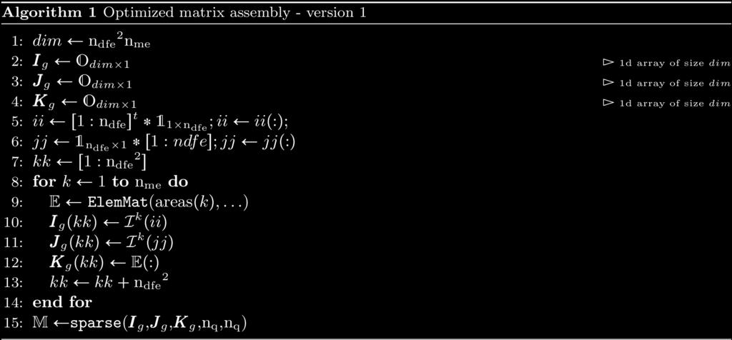
11 1.2 Sparse matrix requirement The interpreted language must contain a function to generate a sparse matrix M from three 1d arrays of same length Ig, Jg and Kg such that M(Ig(k),Jg(k))=Kg(k). Furthermore, the elements of Kg having the same indices in Ig and Jg must be summed. We give for several interpreted languages the corresponding function : Python (scipy.sparse module) : M=sparse.<format>_matrix(Kg,(Ig,Jg),shape=(m,n) where <format> is the sparse matrix format chosen in csc, csr, lil,... Matlab : M=sparse(Ig,Jg,Kg,m,n), only csc format. Octave : M=sparse(Ig,Jg,Kg,m,n), only csc format. Scilab : M=sparse([Ig,Jg],Kg,[m,n]), only row-by-row format. Obviously, this kind of function exists in compiled languages. For example, in C language, one can use the SuiteSparse from T. Davis and with Nvidia GPU, one can use Thrust library. 1.3 Optimized classical assembly algorithm (OptV1 version) The idea is to create three global 1d-arrays I g, J g and K g allowing the storage of the element matrices as well as the position of their elements in the global matrix. The length of each array is n 2 dfe n me. (i.e. 9n me for d = 2 and 16n me for d = 3 ). Once these arrays are created, the matrix assembly is obtained with one of the previous commands. To create these three arrays, we first define three local 1d-arrays K e k, Ie k and J e k of n2 dfe elements obtained from a generic element matrix E(T k ) of dimension n dfe : From these arrays, it is then possible to build the three global arrays I g, J g and K g, of size n 2 dfe n me 1 defined, k {1,..., n me }, l { 1,..., n 2 dfe}, by K(n 2 dfe (k 1) + l) = Ke k (l), I(n 2 dfe (k 1) + l) = Ie k (l) = Ik ((l 1) mod m + 1), J(n 2 dfe (k 1) + l) = J e k (l) = Ik (E((l 1)/m) + 1). So, for each triangle T k, we have Then, a simple algorithm can build these three arrays using a loop over each triangle. Note: We give the complete OptV1 algorithm 1.4 New Optimized assembly algorithm (OptV2 version) We present the optimized version 2 algorithm where no loop is used. We define three 2d-arrays that allow to store all the element matrices as well as their positions in the global matrix. We denote by K g, I g and J g these n 2 dfe by n me 1.2. Sparse matrix requirement 7

12 8 Chapter 1. Presentation

13 arrays, defined k {1,..., n me }, il {1,..., n 2 dfe } by K g (il, k) = K e k(il), I g (il, k) = I e k(il), J g (il, k) = J e k(il). (1.1) The three local arrays K e k, Ie k and J e k are thus stored in the kth column of the global arrays K g, I g and J g respectively. A natural way to build these three arrays consists in using a loop through the triangles T k in which we insert the local arrays column-wise Figure 1.3: Construction of K g, I g and J g with loop The natural construction of these three arrays is done column-wise. So, for each array there are n me columns to compute, which depends on the mesh size. To vectorize, we must fill these arrays by row-wise operations and then for each array there are n 2 dfe rows to compute. We recall that n dfe does not depend on the mesh size. These rows insertions are represented in Figure 1.4. We can also remark that, (α, β) {1,..., n dfe }, with m = n dfe, K g (m(β 1) + α, k) = e k α,β, I g (m(β 1) + α, k) = I k α, J g (m(β 1) + α, k) = I k β New Optimized assembly algorithm (OptV2 version) 9

14 where, in scalar fields case, Iα k = me(α, k), α {1,..., d + 1} and in vector fields case, Ida b k = d me(a, k) b, a {1,..., d + 1}, b {0,..., d 1}. Figure 1.4: Row-wise operations on global arrays I g, J g and K g As we can see in Figures 1.5 and 1.6, it is quite easy to vectorize I g and J g computations in scalar fields case by filling these arrays lines by lines : Figure 1.5: Construction of I g and J g : OptV2 version for 2d scalar matrix Using vectorization tools, we can compute I g and J g in one line. The vectorized algorithms in 2d and 3d scalar fields are represented by Figure 1.7. In vector fields case, we construct the tabular T such that T(α, k) = I k α, α {1,..., n dfe }. Then we can vectorize I g and J g computations in vector fields case. We represent in Figure 1.8 these operations in 2d. Now, it remains to vectorize the computation of K g array which contains all the element matrices associated to D or H : it should be done by row-wise vector operations. We now describe a vectorized construction of K g array associated to a generic bilinear form a. For the mesh element T k, the element matrix is then given by a(φ i k 1, φ i k 1 ) a(φ i k 1, φ i k 2 ) a(φ i k 1, φ i k 3 ) E(T k ) = a(φ i k 2, φ i k 1 ) a(φ i k 2, φ i k 2 ) a(φ i k 2, φ i k 3 ) a(φ i k 3, φ i k 1 ) a(φ i k 3, φ i k 2 ) a(φ i k 3, φ i k 3 ) 10 Chapter 1. Presentation

15 Figure 1.6: Construction of I g and J g : OptV2 version for 3d scalar matrix Figure 1.7: Vectorized algorithms for I g and J g computations 1.4. New Optimized assembly algorithm (OptV2 version) 11

16 Figure 1.8: Construction of I g and J g : OptV2 version in 2d vector fields case 12 Chapter 1. Presentation

17 Figure 1.9: Construction of K g for Mass matrix 1.4. New Optimized assembly algorithm (OptV2 version) 13

18 Figure 1.10: Construction of K g for Mass matrix 14 Chapter 1. Presentation

19 CHAPTER TWO 2D BENCHMARKS Contents Benchmark usage Mass Matrix Stiffness Matrix Elastic Stiffness Matrix 2.1 Benchmark usage pyoptfem.fem2d.assemblybench.assemblybench([assembly=<string>, version=<string>, LN=<array>, meshname=<string>, meshdir=<string>, nbruns=<int>, la=<float>, mu=<float>, Num=<int>, tag=<string>,...]) Benchmark code for P 1 -Lagrange finite element matrices defined in FEM2D. Parameters assembly Name of an assembly routine. The string should be : MassAssembling2DP1, StiffAssembling2DP1 (default) StiffElasAssembling2DP1 versions List of versions. Must be a list of any size whose elements may be { base, OptV1, OptV2 } (default : [ OptV2, OptV1, base ]) meshname Name of the mesh files. By default it is an empty string. It means it uses SquareMesh function to generate meshes. meshdir Directory location of FreeFEM++ mesh files. Used if meshname is not empty. LN array of integer values. <LN> contains the values of N. Used to generate meshes data via Th=SquareMesh(N) function if meshname is empty or via getmesh class to read FreeFEM++ meshes Th=getMesh(meshdir+ / +meshname+str(n)+.msh ) LN default value is range(50, 90, 10) nbruns Number of runs on each mesh (default : 1) save For saving benchmark results in a file (see parameters <output>, <outdir> and <tag>) 15

20 plot For plotting computation times (default : True) output Name used to set results file name (default : bench2d ) outdir Directory location of saved results file name (default :./results ). tag Specify a tag string added to filename la the first Lame coefficient in Hooke s law, denoted by λ. Used by functions for assembling the elastic stiffness matrix. (default : 2) mu the second Lame coefficient in Hooke s law, denoted by μ. Used by functions for assembling the elastic stiffness matrix. (default : 0.3) Num Numbering choice. Used by functions for assembling the elastic stiffness matrix. (default : 0) 2.2 Mass Matrix Benchmark of MassAssembling2DP1 with base, OptV1 and OptV2 versions (see Mass Matrix) Table 2.1: MassAssembling2DP1 benchmark summary N nq ndof OptV2 OptV1 base (s) (s) (s) x1.00 x19.50 x (s) (s) (s) x1.00 x20.02 x (s) (s) (s) x1.00 x20.32 x (s) (s) (s) x1.00 x20.33 x (s) (s) (s) x1.00 x19.66 x (s) (s) (s) x1.00 x19.89 x (s) (s) (s) x1.00 x19.88 x (s) (s) (s) x1.00 x20.21 x This tabular was built with the following code : >>> from pyoptfem.fem2d import assemblybench >>> assemblybench(assembly= MassAssembling2DP1,LN=range(50,130,10)) SquareMesh(50): -> MassAssembling2DP1OptV2(nq=2601, nme=5000) run ( 1/ 1) : cputime= (s) - matrix 2601-by SquareMesh(120): -> MassAssembling2DP1base(nq=14641, nme=28800) run ( 1/ 1) : cputime= (s) - matrix by We also obtain Benchmark of MassAssembling2DP1 with OptV2 and OptV1 versions 16 Chapter 2. 2D benchmarks

21 Figure 2.1: MassAssembling2DP1 benchmark 2.2. Mass Matrix 17

22 Table 2.2: MassAssembling2DP1 benchmark summary N nq ndof OptV2 OptV (s) (s) x1.00 x (s) (s) x1.00 x (s) (s) x1.00 x (s) (s) x1.00 x (s) (s) x1.00 x (s) (s) x1.00 x (s) (s) x1.00 x (s) (s) x1.00 x (s) (s) x1.00 x (s) (s) x1.00 x (s) (s) x1.00 x (s) (s) x1.00 x17.52 This tabular was built with the following code : >>> from pyoptfem.fem2d import assemblybench >>> assemblybench(assembly= MassAssembling2DP1,versions=[ OptV2, OptV1 ],LN=range(100,1300,100 SquareMesh(100): -> MassAssembling2DP1OptV2(nq=10201, nme=20000) run ( 1/ 1) : cputime= (s) - matrix by SquareMesh(1200): -> MassAssembling2DP1OptV1(nq= , nme= ) run ( 1/ 1) : cputime= (s) - matrix by We also obtain 2.3 Stiffness Matrix Benchmark of StiffAssembling2DP1 with base, OptV1 and OptV2 versions 18 Chapter 2. 2D benchmarks

23 Figure 2.2: MassAssembling2DP1 benchmark 2.3. Stiffness Matrix 19

24 Table 2.3: StiffAssembling2DP1 benchmark summary N nq ndof OptV2 OptV1 base (s) (s) (s) x1.00 x45.35 x (s) (s) (s) x1.00 x47.38 x (s) (s) (s) x1.00 x48.33 x (s) (s) (s) x1.00 x46.11 x (s) (s) (s) x1.00 x45.57 x (s) (s) (s) x1.00 x44.77 x (s) (s) (s) x1.00 x45.61 x (s) (s) (s) x1.00 x44.69 x This tabular was built with the following code : >>> from pyoptfem.fem2d import assemblybench >>> assemblybench(assembly= StiffAssembling2DP1,LN=range(50,130,10)) SquareMesh(50): -> StiffAssembling2DP1OptV2(nq=2601, nme=5000) run ( 1/ 1) : cputime= (s) - matrix 2601-by SquareMesh(120): -> StiffAssembling2DP1base(nq=14641, nme=28800) run ( 1/ 1) : cputime= (s) - matrix by We also obtain Benchmark of StiffAssembling2DP1 with OptV2 and OptV1 versions 20 Chapter 2. 2D benchmarks

25 Figure 2.3: StiffAssembling2DP1 benchmark 2.3. Stiffness Matrix 21

26 Table 2.4: StiffAssembling2DP1 benchmark summary N nq ndof OptV2 OptV (s) (s) x1.00 x (s) (s) x1.00 x (s) (s) x1.00 x (s) (s) x1.00 x (s) (s) x1.00 x (s) (s) x1.00 x (s) (s) x1.00 x (s) (s) x1.00 x (s) (s) x1.00 x (s) (s) x1.00 x (s) (s) x1.00 x (s) (s) x1.00 x34.14 This tabular was built with the following code : >>> from pyoptfem.fem2d import assemblybench >>> assemblybench(assembly= StiffAssembling2DP1,versions=[ OptV2, OptV1 ],LN=range(100,1300,10 SquareMesh(100): -> StiffAssembling2DP1OptV2(nq=10201, nme=20000) run ( 1/ 1) : cputime= (s) - matrix by SquareMesh(1200): -> StiffAssembling2DP1OptV1(nq= , nme= ) run ( 1/ 1) : cputime= (s) - matrix by We also obtain 2.4 Elastic Stiffness Matrix Benchmark of StiffElasAssembling2DP1 with base, OptV1 and OptV2 versions 22 Chapter 2. 2D benchmarks

27 Figure 2.4: StiffAssembling2DP1 benchmark 2.4. Elastic Stiffness Matrix 23

28 Table 2.5: StiffElasAssembling2DP1 benchmark summary N nq ndof OptV2 OptV1 base (s) (s) (s) x1.00 x26.29 x (s) (s) (s) x1.00 x28.37 x (s) (s) (s) x1.00 x28.92 x (s) (s) (s) x1.00 x29.26 x (s) (s) (s) x1.00 x29.04 x (s) (s) (s) x1.00 x29.39 x (s) (s) (s) x1.00 x29.21 x This tabular was built with the following code : >>> from pyoptfem.fem2d import assemblybench >>> assemblybench(assembly= StiffElasAssembling2DP1,LN=range(30,65,5)) SquareMesh(30): -> StiffElasAssembling2DP1OptV2(nq=961, nme=1800) run ( 1/ 1) : cputime= (s) - matrix 1922-by SquareMesh(30): -> StiffElasAssembling2DP1OptV2(nq=961, nme=1800) run ( 1/ 1) : cputime= (s) - matrix 1922-by We also obtain Benchmark of StiffElasAssembling2DP1 with OptV2 and OptV1 versions StiffElasAssembling2DP1 benchmark sum- Table 2.6: mary N nq ndof OptV2 OptV (s) (s) x1.00 x (s) (s) x1.00 x (s) (s) x1.00 x (s) (s) x1.00 x (s) (s) x1.00 x (s) (s) x1.00 x (s) (s) x1.00 x (s) (s) x1.00 x Chapter 2. 2D benchmarks

29 Figure 2.5: StiffElasAssembling2DP1 benchmark 2.4. Elastic Stiffness Matrix 25

30 This tabular was built with the following code : >>> from pyoptfem.fem2d import assemblybench >>> assemblybench(assembly= StiffElasAssembling2DP1,versions=[ OptV2, OptV1 ],LN=range(100,900 SquareMesh(100): -> StiffElasAssembling2DP1OptV2(nq=10201, nme=20000) run ( 1/ 1) : cputime= (s) - matrix by SquareMesh(800): -> StiffElasAssembling2DP1OptV1(nq=641601, nme= ) run ( 1/ 1) : cputime= (s) - matrix by We also obtain Figure 2.6: StiffElasAssembling2DP1 benchmark 26 Chapter 2. 2D benchmarks

31 CHAPTER THREE 3D BENCHMARKS Contents Benchmark usage Mass Matrix Stiffness Matrix Elastic Stiffness Matrix 3.1 Benchmark usage pyoptfem.fem3d.assemblybench.assemblybench([assembly=<string>, version=<string>, LN=<array>, meshname=<string>, meshdir=<string>, nbruns=<int>, la=<float>, mu=<float>, Num=<int>, tag=<string>,...]) Benchmark code for P 1 -Lagrange finite element matrices defined in FEM3D. Parameters assembly Name of an assembly routine. The string should be : MassAssembling3DP1, StiffAssembling3DP1 (default) StiffElasAssembling3DP1 versions List of versions. Must be a list of any size whose elements may be { base, OptV1, OptV2 } (default : [ OptV2, OptV1, base ]) meshname Name of the medit mesh files. By default it is an empty string. It means it uses CubeMesh(N) function to generate meshes. meshdir Directory location of medit mesh files. Used if meshname is not empty. LN array of integer values. <LN> contains the values of N. Used to generate meshes data via Th=CubeMesh(N) function if meshname is empty or via getmesh class to read FreeFEM++ meshes Th=getMesh(meshdir+ / +meshname+str(n)+.mesh ) LN default value is range(5, 14, 2) nbruns Number of runs on each mesh (default : 1) save For saving benchmark results in a file (see parameters <output>, <outdir> and <tag>). (default : False) 27

32 plot For plotting computation times (default : True) output Name used to set results file name (default : bench2d ) outdir Directory location of saved results file name (default :./results ). tag Specify a tag string added to filename la the first Lame coefficient in Hooke s law, denoted by λ. Used by functions for assembling the elastic stiffness matrix. (default : 2) mu the second Lame coefficient in Hooke s law, denoted by μ. Used by functions for assembling the elastic stiffness matrix. (default : 0.3) Num Numbering choice. Used by functions for assembling the elastic stiffness matrix. (default : 0) 3.2 Mass Matrix Benchmark of MassAssembling3DP1 with base, OptV1 and OptV2 versions (see Mass Matrix) Table 3.1: MassAssembling23P1 benchmark summary N nq ndof OptV2 OptV1 base (s) (s) (s) x1.00 x28.29 x (s) (s) (s) x1.00 x44.96 x (s) (s) (s) x1.00 x42.55 x (s) (s) (s) x1.00 x40.26 x (s) (s) (s) x1.00 x36.38 x (s) (s) (s) x1.00 x36.99 x (s) (s) (s) x1.00 x35.57 x This tabular was built with the following code : >>> from pyoptfem.fem3d import assemblybench >>> assemblybench(assembly= MassAssembling3DP1,LN=range(5,40,5)) CubeMesh(5): -> MassAssembling3DP1OptV2(nq=216, nme=750) run ( 1/ 1) : cputime= (s) - matrix 216-by CubeMesh(35): -> MassAssembling3DP1base(nq=46656, nme=257250) run ( 1/ 1) : cputime= (s) - matrix by We also obtain Benchmark of MassAssembling3DP1 with OptV2 and OptV1 versions 28 Chapter 3. 3D benchmarks

33 Figure 3.1: MassAssembling3DP1 benchmark 3.2. Mass Matrix 29

34 Table 3.2: MassAssembling2DP1 benchmark summary N nq ndof OptV2 OptV (s) (s) x1.00 x (s) (s) x1.00 x (s) (s) x1.00 x (s) (s) x1.00 x (s) (s) x1.00 x (s) (s) x1.00 x (s) (s) x1.00 x (s) (s) x1.00 x (s) (s) x1.00 x (s) (s) x1.00 x34.71 This tabular was built with the following code : >>> from pyoptfem.fem3d import assemblybench >>> assemblybench(assembly= MassAssembling3DP1,versions=[ OptV2, OptV1 ],LN=range(10,110,10)) CubeMesh(10): -> MassAssembling3DP1OptV2(nq=1331, nme=6000) run ( 1/ 1) : cputime= (s) - matrix 1331-by CubeMesh(100): -> MassAssembling3DP1OptV1(nq= , nme= ) run ( 1/ 1) : cputime= (s) - matrix by We also obtain 3.3 Stiffness Matrix Benchmark of StiffAssembling3DP1 with base, OptV1 and OptV2 versions 30 Chapter 3. 3D benchmarks

35 Figure 3.2: MassAssembling3DP1 benchmark 3.3. Stiffness Matrix 31

36 Table 3.3: StiffAssembling3DP1 benchmark summary N nq ndof OptV2 OptV1 base (s) (s) (s) x1.00 x23.22 x (s) (s) (s) x1.00 x60.68 x (s) (s) (s) x1.00 x58.08 x (s) (s) (s) x1.00 x53.55 x (s) (s) (s) x1.00 x51.61 x (s) (s) (s) x1.00 x47.85 x (s) (s) (s) x1.00 x44.37 x This tabular was built with the following code : >>> from pyoptfem.fem3d import assemblybench >>> assemblybench(assembly= StiffAssembling3DP1,LN=range(5,40,5)) CubeMesh(5): -> StiffAssembling3DP1OptV2(nq=216, nme=750) run ( 1/ 1) : cputime= (s) - matrix 216-by CubeMesh(35): -> StiffAssembling3DP1base(nq=46656, nme=257250) run ( 1/ 1) : cputime= (s) - matrix by We also obtain Benchmark of StiffAssembling3DP1 with OptV2 and OptV1 versions 32 Chapter 3. 3D benchmarks

37 Figure 3.3: StiffAssembling3DP1 benchmark 3.3. Stiffness Matrix 33

38 Table 3.4: StiffAssembling3DP1 benchmark summary N nq ndof OptV2 OptV (s) (s) x1.00 x (s) (s) x1.00 x (s) (s) x1.00 x (s) (s) x1.00 x (s) (s) x1.00 x (s) (s) x1.00 x (s) (s) x1.00 x (s) (s) x1.00 x (s) (s) x1.00 x (s) (s) x1.00 x29.04 This tabular was built with the following code : >>> from pyoptfem.fem3d import assemblybench >>> assemblybench(assembly= StiffAssembling3DP1,versions=[ OptV2, OptV1 ],LN=range(10,110,10)) CubeMesh(10): -> StiffAssembling3DP1OptV2(nq=1331, nme=6000) run ( 1/ 1) : cputime= (s) - matrix 1331-by CubeMesh(100): -> StiffAssembling3DP1OptV1(nq= , nme= ) run ( 1/ 1) : cputime= (s) - matrix by We also obtain 3.4 Elastic Stiffness Matrix Benchmark of StiffAssembling3DP1 with base, OptV1 and OptV2 versions 34 Chapter 3. 3D benchmarks

39 Figure 3.4: StiffAssembling3DP1 benchmark 3.4. Elastic Stiffness Matrix 35

40 Table 3.5: StiffAssembling3DP1 benchmark summary N nq ndof OptV2 OptV1 base (s) (s) (s) x1.00 x11.23 x (s) (s) (s) x1.00 x33.87 x (s) (s) (s) x1.00 x43.43 x (s) (s) (s) x1.00 x46.91 x (s) (s) (s) x1.00 x47.89 x (s) (s) (s) x1.00 x46.86 x (s) (s) (s) x1.00 x43.22 x This tabular was built with the following code : >>> from pyoptfem.fem3d import assemblybench >>> from numpy import * >>> assemblybench(assembly= StiffElasAssembling3DP1,LN=array([3,5,7,10,13,17,20])) CubeMesh(3): -> StiffElasAssembling3DP1OptV2(nq=64, nme=162) run ( 1/ 1) : cputime= (s) - matrix 192-by CubeMesh(20): -> StiffElasAssembling3DP1base(nq=9261, nme=48000) run ( 1/ 1) : cputime= (s) - matrix by We also obtain Benchmark of StiffAssembling3DP1 with OptV1 and OptV2 versions Table 3.6: StiffAssembling3DP1 benchmark summary N nq ndof OptV2 OptV (s) (s) x1.00 x (s) (s) x1.00 x (s) (s) x1.00 x (s) (s) x1.00 x (s) (s) x1.00 x (s) (s) x1.00 x (s) (s) x1.00 x27.88 This tabular was built with the following code : 36 Chapter 3. 3D benchmarks

41 Figure 3.5: StiffElasAssembling3DP1 benchmark 3.4. Elastic Stiffness Matrix 37

42 >>> from pyoptfem.fem3d import assemblybench >>> assemblybench(assembly= StiffElasAssembling3DP1,versions=[ OptV2, OptV1 ],LN=range(10,80,1 CubeMesh(10): -> StiffElasAssembling3DP1OptV2(nq=1331, nme=6000) run ( 1/ 1) : cputime= (s) - matrix 3993-by CubeMesh(70): -> StiffElasAssembling3DP1OptV1(nq=357911, nme= ) run ( 1/ 1) : cputime= (s) - matrix by We also obtain Figure 3.6: StiffElasAssembling3DP1 benchmark 38 Chapter 3. 3D benchmarks

43 CHAPTER FOUR FEM2D MODULE Author Francois Cuvelier Date 15/09/2013 Contains functions to build some finite element matrices using P 1 -Lagrange finite elements on a 2D mesh. Each assembly matrix is computed by three different versions called base, OptV1 and OptV2 (see here) Contents Assembly matrices (base, OptV1 and OptV2 versions) Mass Matrix Stiffness Matrix Elastic Stiffness Matrix Element matrices (used by base and OptV1 versions) Element Mass Matrix Element Stiffness Matrix Element Elastic Stiffness Matrix Vectorized tools (used by OptV2 version) Vectorized computation of basis functions gradients Vectorized element matrices (used by OptV2 version) Element Mass Matrix Element Stiffness Matrix Element Elastic Stiffness Matrix Mesh 39

44 4.1 Assembly matrices (base, OptV1 and OptV2 versions) Let T h be a triangular mesh of Ω. We denote by Ω h structure: = T k T h T k a triangulation of Ω with the following data name type dimension description Python n q integer 1 number of vertices nq n me integer 1 number of elements nme q double 2 n q array of vertices coordinates. q(ν, j) is the ν-th coordinate of the j-th vertex, ν {1, 2}, j {1,..., n q }. The j-th vertex will be also denoted by q j me integer 3 n me connectivity array. me(β, k) is the storage index of the β-th vertex of the k-th element, in the array q, for β {1, 2, 3} and k {1,..., n me } areas double 1 n me array of areas. areas(k) is the k-th triangle area, k {1,..., n me } q (transposed) q[j-1] = q j me (transposed) areas The P 1 -Lagrange basis functions associated to Ω h are denoted by φ i for all i {1,..., n q } and defined by φ i (q j ) = δ i,j, (i, j) {1,..., n q } 2 We also define the global alternate basis B a by B a = {ψ 1,..., ψ 2nq } = { ( φ1 0 ), ( ) 0, φ 1 ( ) ( ) ( ) ( ) } φ2 0 φnq 0,,...,, 0 φ 2 0 φ nq and the global block basis B b by B b = {φ 1,..., φ 2nq } = { ( ) ( ) ( ) ( ( ( ) } φ1 φ2 φnq 0 0 0,,...,,,,..., φ1) φ2) φ nq Mass Matrix Assembly of the Mass Matrix by P 1 -Lagrange finite elements using base, OptV1 and OptV2 versions respectively (see report). The Mass Matrix M is given by M i,j = φ j (q) φ i (q)dq, (i, j) {1,..., n q } 2. Ω h Note: generic syntax: M = MassAssembling2DP1<version>(nq,nme,me,areas) nq: total number of nodes of the mesh, also denoted by n q, nme: total number of triangles, also denoted by n me, 40 Chapter 4. FEM2D module

45 me: Connectivity array, (nme,3) array, areas: Array of areas, (nme,) array, returns a Scipy CSC sparse matrix of size n q n q where <version> is base, OptV1 or OptV2 Benchmarks of theses functions are presented in Mass Matrix. We give a simple usage : >>> from pyoptfem.fem2d import * >>> Th=SquareMesh(5) >>> Mbase = MassAssembling2DP1base(Th.nq,Th.nme,Th.me,Th.areas) >>> MOptV1= MassAssembling2DP1OptV1(Th.nq,Th.nme,Th.me,Th.areas) >>> print(" NormInf(Mbase-MOptV1)=%e " % NormInf(Mbase-MOptV1)) NormInf(Mbase-MOptV1)= e-18 >>> MOptV2= MassAssembling2DP1OptV2(Th.nq,Th.nme,Th.me,Th.areas) >>> print(" NormInf(Mbase-MOptV2)=%e " % NormInf(Mbase-MOptV2)) NormInf(Mbase-MOptV2)= e-18 We can show sparsity of the Mass matrix : >>> from pyoptfem.fem2d import * >>> Th=SquareMesh(20) >>> M=MassAssembling2DP1base(Th.nq,Th.nme,Th.me,Th.areas) >>> showsparsity(m) Note: source code pyoptfem.fem2d.assembly.massassembling2dp1base(nq, nme, me, areas) Assembly of the Mass Matrix by P 1 -Lagrange finite elements using base version (see report). pyoptfem.fem2d.assembly.massassembling2dp1optv1(nq, nme, me, areas) Assembly of the Mass Matrix by P 1 -Lagrange finite elements using OptV1 version (see report). pyoptfem.fem2d.assembly.massassembling2dp1optv2(nq, nme, me, areas) Assembly of the Mass Matrix by P 1 -Lagrange finite elements using OptV2 version (see report) Stiffness Matrix Assembly of the Stiffness Matrix by P 1 -Lagrange finite elements using base, OptV1 and OptV2 versions respectively (see report). The Stiffness Matrix S is given by S i,j = φ j (q). φ i (q)dq, (i, j) {1,..., n q } 2. Ω h Note: generic syntax: M = StiffAssembling2DP1<version>(nq,nme,q,me,areas) nq: total number of nodes of the mesh, also denoted by n q, nme: total number of triangles, also denoted by n me, q: Array of vertices coordinates, (nq,2) array 4.1. Assembly matrices (base, OptV1 and OptV2 versions) 41

46 Figure 4.1: Sparsity of Mass Matrix generated with command showsparsity(m) 42 Chapter 4. FEM2D module

47 me: Connectivity array, (nme,3) array, areas: Array of areas, (nme,) array, returns a Scipy CSC sparse matrix of size n q n q where <version> is base, OptV1 or OptV2 Benchmarks of theses functions are presented in Stiffness Matrix. We give a simple usage : >>> pyoptfem.fem2d import * >>> Th=SquareMesh(5) >>> Sbase = StiffAssembling2DP1base(Th.nq,Th.nme,Th.q,Th.me,Th.areas) >>> SOptV1= StiffAssembling2DP1OptV1(Th.nq,Th.nme,Th.q,Th.me,Th.areas) >>> print(" NormInf(Sbase-SOptV1)=%e " % NormInf(Sbase-SOptV1)) NormInf(Sbase-SOptV1)= e+00 >>> SOptV2= StiffAssembling2DP1OptV2(Th.nq,Th.nme,Th.q,Th.me,Th.areas) >>> print(" NormInf(Sbase-SOptV2)=%e " % NormInf(Sbase-SOptV2)) NormInf(Sbase-SOptV1)= e-16 Note: source code pyoptfem.fem2d.assembly.stiffassembling2dp1base(nq, nme, q, me, areas) Assembly of the Stiffness Matrix by P 1 -Lagrange finite elements using base version (see report). pyoptfem.fem2d.assembly.stiffassembling2dp1optv1(nq, nme, q, me, areas) Assembly of the Stiffness Matrix by P 1 -Lagrange finite elements using OptV1 version (see report). pyoptfem.fem2d.assembly.stiffassembling2dp1optv2(nq, nme, q, me, areas) Assembly of the Stiffness Matrix by P 1 -Lagrange finite elements using OptV2 version (see report) Elastic Stiffness Matrix Assembly of the Elastic Stiffness Matrix by P 1 -Lagrange finite elements using base, OptV1 and OptV2 versions respectively (see report). The Elastic Stiffness Matrix K is given by K m,l = ε t (ψ l (q))σ(ψ m (q)), (m, l) {1,..., 2n q } 2. Ω h where σ = (σ xx, σ yy, σ xy ) t and ε = (ε xx, ε yy, ε xy ) t are the elastic stress and strain tensors respectively. Note: generic syntax: M = StiffElasAssembling2DP1<version>(nq,nme,q,me,areas,la,mu,Num) nq: total number of nodes of the mesh, also denoted by n q, nme: total number of triangles, also denoted by n me, q: array of vertices coordinates, (nq,2) array for base and OptV1, (2,nq) array for OptV2 version, me: Connectivity array, (nme,3) array for base and OptV1, 4.1. Assembly matrices (base, OptV1 and OptV2 versions) 43

48 (3,nme) array for OptV2 version, areas: (nme,) array of areas, la: the first Lame coefficient in Hooke s law, denoted by λ, mu: the second Lame coefficient in Hooke s law, denoted by μ, Num: 0: global alternate numbering with local alternate numbering (classical method), 1: global block numbering with local alternate numbering, 2: global alternate numbering with local block numbering, 3: global block numbering with local block numbering. returns a Scipy CSC sparse matrix of size 2n q 2n q where <version> is base, OptV1 or OptV2 Benchmarks of theses functions are presented in Elastic Stiffness Matrix. We give a simple usage : >>> from pyoptfem.fem2d import * >>> Th=SquareMesh(5) >>> Kbase = StiffElasAssembling2DP1base(Th.nq,Th.nme,Th.q,Th.me,Th.areas,2,0.5,0) >>> KOptV1= StiffElasAssembling2DP1OptV1(Th.nq,Th.nme,Th.q,Th.me,Th.areas,2,0.5,0) >>> print(" NormInf(Kbase-KOptV1)=%e " % NormInf(Kbase-KOptV1)) NormInf(Kbase-KOptV1)= e-16 >>> KOptV2= StiffElasAssembling2DP1OptV2(Th.nq,Th.nme,Th.q,Th.me,Th.areas,2,0.5,0) >>> print(" NormInf(Kbase-KOptV2)=%e " % NormInf(Kbase-KOptV2)) NormInf(Kbase-KOptV2)= e-15 We now illustrate the consequences of the choice of the global basis on matrix sparsity global alternate basis B a (Num=0 or Num=2) >>> from pyoptfem.fem2d import * >>> Th=SquareMesh(15) >>> K0=StiffElasAssembling2DP1OptV1(Th.nq,Th.nme,Th.q,Th.me,Th.areas,2,0.5,0) >>> showsparsity(k0) >>> K3=StiffElasAssembling2DP1OptV1(Th.nq,Th.nme,Th.q,Th.me,Th.areas,2,0.5,3) >>> showsparsity(k3) global block basis B a (Num=1 or Num=3) Note: source code pyoptfem.fem2d.assembly.stiffelasassembling2dp1base(nq, nme, q, me, areas, la, mu, Num) Assembly of the Elasticity Stiffness Matrix by P 1 -Lagrange finite elements using OptV2 version (see report). pyoptfem.fem2d.assembly.stiffelasassembling2dp1optv1(nq, nme, q, me, areas, la, mu, Num) Assembly of the Elasticity Stiffness Matrix by P 1 -Lagrange finite elements using OptV1 version (see report). pyoptfem.fem2d.assembly.stiffelasassembling2dp1optv2(nq, nme, q, me, areas, la, mu, Num) Assembly of the Elasticity Stiffness Matrix by P 1 -Lagrange finite elements using OptV2 version (see report). 44 Chapter 4. FEM2D module

49 Figure 4.2: Sparsity of the Elastic Stiffness Matrix generated with global alternate numbering (Num=0 or 2) 4.1. Assembly matrices (base, OptV1 and OptV2 versions) 45

50 Figure 4.3: Sparsity of the Elastic Stiffness Matrix generated with global block numbering (Num=1 or 3) 46 Chapter 4. FEM2D module

51 4.2 Element matrices (used by base and OptV1 versions) Let T be a triangle, of area T and with q 1, q 2 and q 3 its three vertices. We denote by φ 1, φ 2 and φ 3 the P 1 -Lagrange local basis functions such that φ i (q j ) = δ i,j, (i, j) {1, 2, 3} 2. We also define the local alternate basis B a by B a = { ψ ψ ψ1,..., ψ ψ ψ6 } = { ( φ1 0 ) (,, 0 φ1) ( ) ( φ2,, 0 0 φ2) ( ) ( φ3 0 φ3) }, 0 and the local block basis B b by { ( ) B b = { φ φ φ1,..., φ φ φ6 φ1 } =, 0 ( ) φ2, 0 ( ) ( ( ( φ3 0 φ3) },,,. 0 0 φ1) 0 φ2) The elasticity tensor, H, obtained from Hooke s law with an isotropic material, defined with the Lamé parameters λ and μ is given by λ + 2μ λ 0 H = λ λ + 2μ μ and, for a function u = (u 1, u 2 ) the strain tensors is given by ( u1 ε(u) = x, u 2 y, u 2 x + u 1 y ) t Element Mass Matrix The element Mass matrix M e (T ) for the triangle T is defined by M e i,j(t ) = φ i (q) φ j (q) dq, (i, j) {1, 2, 3} 2 T We obtain : M e (T ) = T (4.1) Note: pyoptfem.fem2d.elemmatrix.elemmassmat2dp1(area) Computes the element mass matrix M e (T ) for a given triangle T of area T Parameters area (float) area of the triangle. Returns 3 3 numpy array of floats Element matrices (used by base and OptV1 versions) 47

52 4.2.2 Element Stiffness Matrix The element stiffness matrix, S e (T ), for the T is defined by S e i,j(t ) = < φ i (q), φ j (q) > dq, (i, j) {1, 2, 3} 2 T We have : S e (T ) = 1 4 T < u, u > < u, v > < u, w > < v, u > < v, v > < v, w >. < w, u > < w, v > < w, w > where u = q 2 q 3, v = q 3 q 1 and w = q 1 q 2. Note: pyoptfem.fem2d.elemmatrix.elemstiffmat2dp1(q1, q2, q3, area) Computes the element stiffness matrix S e (T ) for a given triangle T Parameters Returns Type q1,q2,q3 (2 1 numpy array) the three vertices of the triangle, area (float) area of the triangle. 3 3 numpy array of floats Element Elastic Stiffness Matrix Let u = q 2 q 3, v = q 3 q 1 and w = q 1 q 2. The element elastic stiffness matrix, K e (T ), for a given triangle T in the local alternate basis B a is defined by K e i,j(t ) = ε( ψ j ) t (q)hε( ψ i )(q) dq, (i, j) {1,..., 6} 2. T We also have K e (T ) = 1 4 T Bt HB where H is the elasticity tensor and B = u 2 0 v 2 0 w u 1 0 v 1 0 w 1 u 1 u 2 v 1 v 2 w 1 w 2 Note: 48 Chapter 4. FEM2D module

53 pyoptfem.fem2d.elemmatrix.elemstiffelasmat2dp1ba(ql, area, H) Returns the element elastic stiffness matrix K e (T ) for a given triangle T in the local alternate basis B a Parameters ql (3 2 numpy array) contains the three vertices of the triangle : ql[0], ql[1] and ql[2], area (float) area of the triangle, H (3 3 numpy array) Elasticity tensor, H. Returns K e (T ) in B a basis. Type 6 6 numpy array of floats. The element elastic stiffness matrix, K e (T ), for a given triangle T in the local block basis B b is defined by K e i,j(t ) = ε( φ j ) t (q)hε( φ i )(q) dq, (i, j) {1,..., 6} 2. T We also have K e (T ) = 1 4 T Bt HB where H is the elasticity tensor and u 2 v 2 w B = u 1 v 1 w 1 u 1 v 1 w 1 u 2 v 2 w 2 Note: pyoptfem.fem2d.elemmatrix.elemstiffelasmat2dp1bb(ql, area, H) Returns the element elastic stiffness matrix K e (T ) for a given triangle T in the local block basis B b Parameters ql (3 2 numpy array) contains the three vertices of the triangle : ql[0], ql[1] and ql[2], area (float) area of the triangle, H (3 3 numpy array) Elasticity tensor, H. Returns K e (T ) in B b basis. Type 6 6 numpy array of floats 4.2. Element matrices (used by base and OptV1 versions) 49

54 4.3 Vectorized tools (used by OptV2 version) Vectorized computation of basis functions gradients By construction, the gradients of basis functions are constants on each element T k. So, we denote, α {1,..., 3}, by G α the 2 n me array defined, k {1,..., n me }, by G α (:, k) = φ me(α,k) (q), q T k. On a triangle T k, we define D 12 = q me(1,k) q me(2,k), D 13 = q me(1,k) q me(3,k) and D 23 = q me(2,k) q me(3,k). Then, we have φ k 1(q) = 1 ( ) D 23 y 2 T k D 23, φ k 2(q) = 1 ( ) D 13 y x 2 T k D 13, φ k 3(q) = 1 ( ) D 12 y x 2 T k D 12. x With these formulas, we obtain the vectorized algorithm given in Algorithm 4.4. Algorithm 4.4 Figure 4.4: Vectorized algorithm for computation of basis functions gradients in 2d 50 Chapter 4. FEM2D module

55 4.4 Vectorized element matrices (used by OptV2 version) Element Mass Matrix We have M e (T k ) = T k Then with K g definition (see Section New Optimized assembly algorithm (OptV2 version)), we obtain K g (3(i 1) + j, k) = T k 1 + δ i,j 12 1 i, j 3, We represent in figure 4.5 the corresponding row-wise operations. Figure 4.5: Construction of K g associated to 2d Mass matrix in So the vectorized algorithm for K g computation is simple and given in Algorithm 4.6. Algorithm 4.6 Note: pyoptfem.fem2d.elemmatrixvec.elemmassmat2dp1vec(areas) Computes all the element Mass matrices M e (T k ) for k {0,..., n me 1} Parameters areas (n me numpy array of floats) areas of all the mesh elements Vectorized element matrices (used by OptV2 version) 51

56 Figure 4.6: Vectorized algorithm for K g associated to 2d Mass matrix Returns a one dimensional numpy array of size 9n me Element Stiffness Matrix We have (α, β) {1,..., 3} 2 S e α,β(t k ) = T k φ k β, φ k α. Using vectorized algorithm function GRADIENTVEC2D given in Algorithm 4.4, we obtain the vectorized algorithm 4.7 for K g computation for the Stiffness matrix in 2d. Algorithm 4.7 Figure 4.7: Vectorized algorithm for K g associated to 2d Stiffness matrix Note: pyoptfem.fem2d.elemmatrixvec.elemstiffmat2dp1vec(nme, q, me, areas) Computes all the element stiffness matrices S e (T k ) for k {0,..., n me 1} Parameters nme (int) number of mesh elements, q (n q 2 numpy array of floats) mesh vertices, me (n me 3 numpy array of integers) mesh connectivity, 52 Chapter 4. FEM2D module

57 areas (n me numpy array of floats) areas of all the mesh elements. Returns a one dimensional numpy array of size 9n me Element Elastic Stiffness Matrix We define on T k the local alternate basis B k a by B k a = {ψ k 1,..., ψ k 6} = { ( φ k 1 0 ) ( ) ( ) ( ) ( ) ( ) } 0 φ k, φ k, 2 0 φ k, 1 0 φ k, 3 0, 2 0 φ k 3 where φ k α = φ me(α,k). With notations of Presentation, we have (α, β) {1,..., 6} 2 K e α,β(t k ) = ε t (ψ k β)cε(ψ k α)dq = T k H(ψ k β, ψ k α)(q)dq T k with, u = (u 1, u 2 ) H 1 (Ω) 2, v = (v 1, v 2 ) H 1 (Ω) 2, ( ) γ 0 H(u, v) = 0 μ u 1, v 1 ( ) 0 μ + λ 0 u 1, v 2 + ( 0 + ) λ μ 0 u 2, v 1 ) (4.2) u 2, v 2 ( μ 0 0 γ For example, we can explicitly compute the first two terms in the first column of K e (T k ) which are given by K e 1,1(T k ) = T k H(ψ k 1, ψ k 1)(q)dq = ( ( ) ( ) ) φ k T k H 1 φ k, 1 (q)dq ( 0 ) 0 γ 0 = T k 0 μ φ k 1, φ k 1 = T k ( γ φk 1 φ k 1 x x + μ φk 1 y ) φ k 1 y. and K e 2,1(T k ) = T k H(ψ k 1, ψ k 2)(q)dq = ( ( ) ( ) ) φ k T k H 1 0, 0 φ k (q)dq ( ) 1 0 μ = T k λ 0 φ k 1, φ k 1 = T k (λ + μ) φk 1 x φ k 1 y. Using vectorized algorithm function GRADIENTVEC2D given in Algorithm 4.4, we obtain the vectorized algorithm 4.7 for K g computation for the Elastic Stiffness matrix in 2d. Algorithm 4.8 Note: pyoptfem.fem2d.elemmatrixvec.elemstiffelasmatbavec2dp1(nme, q, me, areas, L, M, **kwargs) Computes all the element elastic stiffness matrices K e (T k ) for k {0,..., n me 1} in local alternate basis Vectorized element matrices (used by OptV2 version) 53

58 Figure 4.8: Vectorized algorithm for K g associated to 2d Elastic Stiffness matrix Parameters nme (int) number of mesh elements, q ((2,nq) numpy array of floats) mesh vertices, me ((3,nme) numpy array of integers) mesh connectivity, areas ((nme,) numpy array of floats) areas of all the mesh elements. L (float) the λ Lame parameter, M (float) the μ Lame parameter. Returns a (36*nme,) numpy array of floats. We define on T k the local block basis Bb k by { ( ) ( ) ( ) ( ) ( ) ( ) } Bb k = {φ k 1,..., φ k φ k 6} = 1 φ k, 2 φ k, , φ k, 1 φ k, 2 φ k 3 where φ k α = φ me(α,k). For example, using formula (4.2), we can explicitly compute the first two terms in the first column of K e (T k ) which are given by K e 1,1(T k ) = T k H(φ k 1, φ k 1)(q)dq = ( ( ) ( ) ) φ k T k H 1 φ k, 1 (q)dq ( 0 ) 0 γ 0 = T k 0 μ φ k 1, φ k 1 = T k ( γ φk 1 φ k 1 x x + μ φk 1 y ) φ k 1 y. 54 Chapter 4. FEM2D module

59 and K e 2,1(T k ) = T k H(φ k 1, φ k 2)(q)dq = ( ( ) ( ) ) φ k T k H 1 φ k, 2 (q)dq ( 0 ) 0 γ 0 = T k 0 μ φ k 1, φ k 2 = T k ( γ φk 1 φ k 2 x x + μ φk 1 y ) φ k 2 y. Using vectorized algorithm function GRADIENTVEC2D given in Algorithm 4.4, we obtain the vectorized algorithm 4.9 for K g computation for the Elastic Stiffness matrix in 2d. Algorithm 4.9 Figure 4.9: Vectorized algorithm for K g associated to 2d Elastic Stiffness matrix Note: pyoptfem.fem2d.elemmatrixvec.elemstiffelasmatbbvec2dp1(nme, q, me, areas, L, M, **kwargs) Computes all the element elastic stiffness matrices K e (T k ) for k {0,..., n me 1} in local block basis. Parameters nme (int) number of mesh elements, q ((2,nq) numpy array of floats) mesh vertices, me ((3,nme) numpy array of integers) mesh connectivity, areas ((nme,) numpy array of floats) areas of all the mesh elements. L (float) the λ Lame parameter, M (float) the μ Lame parameter. Returns a (36*nme,) numpy array of floats Vectorized element matrices (used by OptV2 version) 55

60 4.5 Mesh class pyoptfem.fem2d.mesh.squaremesh(n, **kwargs) Creates meshes of the unit square [0, 1] [0, 1]. Class attributes are : nq, total number of mesh vertices (points), also denoted n q. nme, total number of mesh elements (triangles in 2d), version, mesh structure version, q, Numpy array of vertices coordinates, dimension (nq,2) (version 0) or (2,nq) (version 1). q[j] (version 0) or q[:,j] (version 1) are the two coordinates of the j-th vertex, j {0,.., nq 1} me, Numpy connectivity array, dimension (nme,3) (version 0) or (3,nme) (version 1). me[k] (version 0) or me[:,k] (version 1) are the storage index of the three vertices of the k-th triangle in the array q of vertices coordinates, k {0,..., nme 1}. areas, Array of mesh elements areas, (nme,) Numpy array. areas[k] is the area of k-th triangle, k in range(0,nme) Parameters N number of points on each side of the square optional parameter : version=0 or version=1 >>> from pyoptfem.fem2d import * >>> Th=SquareMesh(3) >>> Th.nme,Th.nq (18, 16) >>> Th.q array([[ 0., 0. ], [ , 0. ], [ , 0. ], [ 1., 0. ], [ 0., ], [ , ], [ , ], [ 1., ], [ 0., ], [ , ], [ , ], [ 1., ], [ 0., 1. ], [ , 1. ], [ , 1. ], [ 1., 1. ]]) >>> PlotMesh(Th) class pyoptfem.fem2d.mesh.getmesh(meshfile, **kwargs) Reads a FreeFEM++ mesh from file meshfile. Class attributes are : nq, total number of mesh vertices (points), also denoted n q. nme, total number of mesh elements (triangles in 2d), version, mesh structure version, q, Numpy array of vertices coordinates, dimension (nq,2) (version 0) or (2,nq) (version 1). q[j] (version 0) or q[:,j] (version 1) are the two coordinates of the j-th vertex, j {0,.., nq 1} 56 Chapter 4. FEM2D module

61 Figure 4.10: SquareMesh(3) visualisation 4.5. Mesh 57

62 me, Numpy connectivity array, dimension (nme,3) (version 0) or (3,nme) (version 1). me[k] (version 0) or me[:,k] (version 1) are the storage index of the three vertices of the k-th triangle in the array q of vertices coordinates, k {0,..., nme 1}. areas, Array of mesh elements areas, (nme,) Numpy array. areas[k] is the area of k-th triangle, k in range(0,nme) Parameters N number of points on each side of the square optional parameter : version=0 or version=1 >>> from pyoptfem.fem2d import * >>> Th=getMesh( mesh/disk4-1-5.msh ) >>> PlotMesh(Th) Figure 4.11: Visualisation of a FreeFEM++ mesh (disk unit) 58 Chapter 4. FEM2D module

63 CHAPTER FIVE FEM3D MODULE Author Francois Cuvelier Date 15/09/2013 Contains functions to build some finite element matrices using P 1 -Lagrange finite elements on a 3D mesh. Each assembly matrix is computed by three differents versions called base, OptV1 and OptV2 (see here) Contents Assembly matrix (base, OptV1 and OptV2 versions) Mass Matrix Stiffness Matrix Elastic Stiffness Matrix Element matrix (used by base and OptV1 versions) Element Mass Matrix Element Stiffness Matrix Element Elastic Stiffness Matrix Vectorized tools (used by OptV2 version) Vectorized computation of basis functions gradients Vectorized element matrix (used by OptV2 version) Element Mass Matrix Element Stiffness Matrix Element Elastic Stiffness Matrix Mesh 59

64 5.1 Assembly matrix (base, OptV1 and OptV2 versions) Let Ω h be a tetrahedral mesh of Ω corresponding to the following structure data: name type dimension description Python n q integer 1 number of vertices nq n me integer 1 number of elements nme q double 3 n q array of vertices coordinates. q(ν, j) is the ν-th coordinate of the j-th vertex, ν {1, 2, 3}, j {1,..., n q }. The j-th vertex will be also denoted by q j me integer 4 n me connectivity array. me(β, k) is the storage index of the β-th vertex of the k-th element, in the array q, for β {1,..., 4} and k {1,..., n me } volumes double 1 n me array of volumes. volumes(k) is the k-th tetrahedron volume, k {1,..., n me } q (transposed) q[j-1] = q j me (transposed) volumes The P 1 -Lagrange basis functions associated to Ω h are denoted by φ i for all i {1,..., n q } and are defined by φ i (q j ) = δ i,j, (i, j) {1,..., n q } 2 We also define the global alternate basis B a by φ B a = {ψ 1,..., ψ 3nq } = 0, φ 1, 0,..., 0 0 φ 1 φ nq 0 0 0, φ nq, φ nq and the global block basis B b by φ 1 B b = {φ 1,..., φ 3nq } = 0,..., 0 φ nq , φ 1,..., φ nq, φ 1,..., 0 0 φ nq Mass Matrix Assembly of the Mass Matrix by P 1 -Lagrange finite elements using base, OptV1 and OptV2 versions respectively (see report). The Mass Matrix M is given by M i,j = φ j (q) φ i (q)dq, (i, j) {1,..., n q } 2. Ω h Note: generic syntax: M = MassAssembling3DP1<version>(nq,nme,me,volumes) nq: total number of nodes of the mesh, also denoted by n q, nme: total number of tetrahedra, also denoted by n me, 60 Chapter 5. FEM3D module

65 me: Connectivity array, (nme,4) array, volumes: Array of tetrahedra volumes, (nme,) array, returns a Scipy CSC sparse matrix of size n q n q where <version> is base, OptV1 or OptV2 >>> from pyoptfem.fem3d import * >>> Th=CubeMesh(5) >>> Mbase = MassAssembling3DP1base(Th.nq,Th.nme,Th.me,Th.volumes) >>> MOptV1= MassAssembling3DP1OptV1(Th.nq,Th.nme,Th.me,Th.volumes) >>> print(" NormInf(Mbase-MOptV1)=%e " % NormInf(Mbase-MOptV1)) NormInf(Mbase-MOptV1)= e-18 >>> MOptV2= MassAssembling3DP1OptV2(Th.nq,Th.nme,Th.me,Th.volumes) >>> print(" NormInf(Mbase-MOptV2)=%e " % NormInf(Mbase-MOptV2)) NormInf(Mbase-MOptV2)= e-18 We can show sparsity of the Mass matrix : >>> from pyoptfem.fem3d import * >>> Th=CubeMesh(5) >>> M=MassAssembling3DP1OptV2(Th.nq,Th.nme,Th.me,Th.areas) >>> showsparsity(m) Figure 5.1: Sparsity of Mass Matrix generated with command showsparsity(m) 5.1. Assembly matrix (base, OptV1 and OptV2 versions) 61

66 Note: source code pyoptfem.fem3d.assembly.massassembling3dp1base(nq, nme, me, volumes) Assembly of the Mass Matrix by P 1 -Lagrange finite elements using base version (see report). pyoptfem.fem3d.assembly.massassembling3dp1optv1(nq, nme, me, volumes) Assembly of the Mass Matrix by P 1 -Lagrange finite elements using OptV1 version (see report). pyoptfem.fem3d.assembly.massassembling3dp1optv2(nq, nme, me, volumes) Assembly of the Mass Matrix by P 1 -Lagrange finite elements using OptV2 version (see report) Stiffness Matrix Assembly of the Stiffness Matrix by P 1 -Lagrange finite elements using base, OptV1 and OptV2 versions respectively (see report). The Stiffness Matrix S is given by S i,j = φ j (q). φ i (q)dq, (i, j) {1,..., n q } 2. Ω h Note: generic syntax M=StiffAssembling3DP1<version>(nq,nme,q,me,volumes) Compute the stiffness sparse matrix where <version> is base, OptV1 or OptV2 Parameters nq total number of nodes of the mesh, also denoted by n q, nme total number of tetrahedra, also denoted by n me, q (numpy array of float) array of vertices coordinates, (nq,3) array for base and OptV1 versions, (3,nq) array for OptV2 version, me (numpy array of int) Connectivity array, (nme,4) array for base and OptV1 versions, (4,nme) array for OptV2 version, volumes (numpy array of floats,) (nme,) array of tetrahedra volumes, Returns a Scipy CSC sparse matrix of size 2n q 2n q Benchmarks of theses functions are presented in Stiffness Matrix. We give a simple usage : >>> from pyoptfem.fem3d import * >>> Th=CubeMesh(5) >>> Sbase = StiffAssembling3DP1base(Th.nq,Th.nme,Th.q,Th.me,Th.volumes) >>> SOptV1= StiffAssembling3DP1OptV1(Th.nq,Th.nme,Th.q,Th.me,Th.volumes) >>> print(" NormInf(Sbase-SOptV1)=%e " % NormInf(Sbase-SOptV1)) NormInf(Sbase-SOptV1)= e Chapter 5. FEM3D module

67 >>> SOptV2= StiffAssembling3DP1OptV2(Th.nq,Th.nme,Th.q,Th.me,Th.volumes) >>> print(" NormInf(Sbase-SOptV2)=%e " % NormInf(Sbase-SOptV2)) NormInf(Sbase-SOptV2)= e-15 Note: source code pyoptfem.fem3d.assembly.stiffassembling3dp1base(nq, nme, q, me, volumes) Assembly of the Stiffness Matrix by P 1 -Lagrange finite elements using base version (see report). pyoptfem.fem3d.assembly.stiffassembling3dp1optv1(nq, nme, q, me, volumes) Assembly of the Stiffness Matrix by P 1 -Lagrange finite elements using OptV1 version (see report). pyoptfem.fem3d.assembly.stiffassembling3dp1optv2(nq, nme, q, me, volumes) Assembly of the Stiffness Matrix by P 1 -Lagrange finite elements using OptV2 version (see report) Elastic Stiffness Matrix Assembly of the Elastic Stiffness Matrix by P 1 -Lagrange finite elements using base, OptV1 and OptV2 versions respectively (see report). The Elastic Stiffness Matrix K is given by K m,l = ε t (ψ l (q)) σ(ψ m (q)), (m, l) {1,..., 3n q } 2. Ω h where σ = (σ xx, σ yy, σ zz, σ xy, σ yz, σ xz ) t and ε = (ε xx, ε yy, ε zz, 2ε xy, 2ε yz, 2ε xz ) t are the elastic stress and strain tensors respectively. Note: generic syntax M=StiffElasAssembling3DP1<version>(nq,nme,q,me,volumes,la,mu,Num) Compute the elastic stiffness sparse matrix where <version> is base, OptV1 or OptV2 Parameters nq total number of nodes of the mesh, nme total number of tetrahedrons, q (numpy array of float) vertices coordinates, (nq,3) array for base and OptV1 versions, (3,nq) array for OptV2 version, me (numpy array of int) connectivity array, (nme,4) array for base and OptV1 versions, (4,nme) array for OptV2 version, volumes (numpy array of floats,) (nme,) array of tetrahedra volumes, la the first Lame coefficient in Hooke s law, denoted by λ, mu the second Lame coefficient in Hooke s law, denoted by μ, Num 5.1. Assembly matrix (base, OptV1 and OptV2 versions) 63

68 0 global alternate numbering with local alternate numbering (classical method), 1 global block numbering with local alternate numbering, 2 global alternate numbering with local block numbering, 3 global block numbering with local block numbering. Returns a Scipy CSC sparse matrix of size 3nq 3nq >>> from pyoptfem.fem3d import * >>> Th=CubeMesh(5) >>> Kbase = StiffElasAssembling3DP1base(Th.nq,Th.nme,Th.q,Th.me,Th.volumes,2,0.5,0) >>> KOptV1= StiffElasAssembling3DP1OptV1(Th.nq,Th.nme,Th.q,Th.me,Th.volumes,2,0.5,0) >>> print(" NormInf(Kbase-KOptV1)=%e " % NormInf(Kbase-KOptV1)) NormInf(Kbase-KOptV1)= e-15 >>> KOptV2= StiffElasAssembling3DP1OptV2(Th.nq,Th.nme,Th.q,Th.me,Th.volumes,2,0.5,0) >>> print(" NormInf(Kbase-KOptV2)=%e " % NormInf(Kbase-KOptV2)) NormInf(Kbase-KOptV2)= e-15 We now illustrate the consequences of the choice of the global basis on matrix sparsity global alternate basis B a (Num=0 or Num=2) >>> from pyoptfem.fem3d import * >>> Th=CubeMesh(5) >>> K0=StiffElasAssembling3DP1OptV1(Th.nq,Th.nme,Th.q,Th.me,Th.volumes,2,0.5,0) >>> showsparsity(k0) global block basis B a (Num=1 or Num=3) >>> K3=StiffElasAssembling3DP1OptV1(Th.nq,Th.nme,Th.q,Th.me,Th.volumes,2,0.5,3) >>> showsparsity(k3) Note: source code pyoptfem.fem3d.assembly.stiffelasassembling3dp1base(nq, nme, q, me, volumes, la, mu, Num) Assembly of the Elasticity Stiffness Matrix by P 1 -Lagrange finite elements using base version (see report). pyoptfem.fem3d.assembly.stiffelasassembling3dp1optv1(nq, nme, q, me, volumes, la, mu, Num) Assembly of the Elasticity Stiffness Matrix by P 1 -Lagrange finite elements using OptV1 version (see report). pyoptfem.fem3d.assembly.stiffelasassembling3dp1optv2(nq, nme, q, me, volumes, la, mu, Num) Assembly of the Elasticity Stiffness Matrix by P 1 -Lagrange finite elements using OptV2 version (see report). 5.2 Element matrix (used by base and OptV1 versions) Let T be a tetrahedron of volume T and with q 1, q 2, q 3 and q 4 its four vertices. We denote by φ 1, φ 2, φ 3 and φ 4 the P 1 -Lagrange local basis functions such that φ i (q j ) = δ i,j, (i, j) {1,..., 4} Chapter 5. FEM3D module

69 Figure 5.2: Sparsity of the Elastic Stiffness Matrix generated with global alternate numbering (Num=0 or 2) 5.2. Element matrix (used by base and OptV1 versions) 65

70 Figure 5.3: Sparsity of the Elastic Stiffness Matrix generated with global block numbering (Num=1 or 3) 66 Chapter 5. FEM3D module

71 We also define the local alternate basis B a by φ φ B a = { ψ ψ ψ1,..., ψ ψ ψ12 } = 0, φ 1, 0,..., 0, φ 4, 0, 0 0 φ φ 4 and the local block basis B b by φ 1 φ 2 φ 3 φ B b = { φ φ φ1,..., φ φ φ12 } = 0, 0, 0, 0,..., 0, 0, φ 1 φ 2 φ 3 φ 4 The elasticity tensor, H, obtained from Hooke s law with an isotropic material, defined with the Lamé parameters λ and μ is given by λ + 2μ λ λ λ λ + 2μ λ H = λ λ λ + 2μ μ μ μ and, for a function u = (u 1, u 2, u 3 ) the strain tensors is given by ε(u) = ( u1 x, u 2 y, u 3 z, u 2 x + u 1 y, u 2 z + u 3 y, u 1 z + u ) t 3 x Element Mass Matrix The element Mass matrix M e (T ) for the tetrahedron T, is defined by M e i,j(t ) = φ i (q) φ j (q) dq, (i, j) {1, 2, 3, 4} 2 T We obtain : M e (T ) = T Note: source code pyoptfem.fem3d.elemmatrix.elemmassmat3dp1(v) Computes the element mass matrix M e (T ) for a given tetrahedron T of volume T 5.2. Element matrix (used by base and OptV1 versions) 67

72 Parameters V (float) volume of the tetrahedron. Returns 4 4 numpy array of floats Element Stiffness Matrix The element stiffness matrix, S e (T ), for the T is defined by S e i,j(t ) = < φ i (q), φ j (q) > dq, (i, j) {1, 2, 3, 4} 2 T Note: source code pyoptfem.fem3d.elemmatrix.elemstiffmat3dp1(ql, volume) Computes the element stiffness matrix S e (T ) for a given tetrahedron T Parameters Returns Type ql (2 4 numpy array) the four vertices of the tetrahedron, volume (float) volume of the tetrahedron. 4 4 numpy array of floats Element Elastic Stiffness Matrix The element elastic stiffness matrix, K e (T ), for a given tetrahedron T in the local alternate basis B a is defined by K e i,j(t ) = ε( ψ j ) t (q)hε( ψ i )(q) dq, (i, j) {1,..., 12} 2. T We also have K e (T ) = 1 4 T Bt HB where H is the elasticity tensor and B is a 6 12 matrix defined by B = ( ε( ψ 1 ) ε( ψ 2 )... ε( ψ 11 ) ε( ψ 12 ) ) 68 Chapter 5. FEM3D module

73 So in B a basis we obtain φ 1 φ x x 0 0 φ 0 1 φ y y 0 φ φ B = z z φ 1 φ 1 φ y x φ 4 y x 0 φ 0 1 φ 1 z φ 1 z 0 y 0 φ 1 x φ 4 z φ 4 z 0 φ 4 y φ 4 x Note: source code pyoptfem.fem3d.elemmatrix.elemstiffelasmatba3dp1(ql, V, C) Returns the element elastic stiffness matrix K e (T ) for a given tetrahedron T in the local alternate basis B a Parameters ql (4 2 numpy array) contains the four vertices of the tetrahedron, V (float) volume of the tetrahedron H (6 6 numpy array) Elasticity tensor, H. Returns K e (T ) in B a basis. Type numpy array of floats. The element elastic stiffness matrix, K e (T ), for a given triangle T in the local block basis B b is defined by K e i,j(t ) = ε( φ j ) t (q)hε( φ i )(q) dq, (i, j) {1,..., 6} 2. T We also have K e (T ) = 1 4 T Bt HB where H is the elasticity tensor and B is a 6 12 matrix defined by ( B = ε( φ 1 ). ε( φ 2 )... ε( φ 11 ) ). ε( φ 12 ) So in B b basis we obtain φ 1 φ x... 4 x φ φ y... 4 y φ φ B = z... 4 z φ 1 φ y... 4 φ 1 φ y x... 4 x φ φ z... 4 φ 1 φ z y... 4 y φ 1 φ z... 4 φ z φ x... 4 x Note: source code 5.2. Element matrix (used by base and OptV1 versions) 69

74 pyoptfem.fem3d.elemmatrix.elemstiffelasmatbb3dp1(ql, V, C) Returns the element elastic stiffness matrix K e (T ) for a given tetrahedron T in the local block basis B b Parameters ql (4 2 numpy array) contains the four vertices of the tetrahedron, V (float) volume of the tetrahedron H (6 6 numpy array) Elasticity tensor, H. Returns K e (T ) in B b basis. Type numpy array of floats. 5.3 Vectorized tools (used by OptV2 version) Vectorized computation of basis functions gradients By construction, the gradients of basis functions are constants on each element T k. So, we denote, α {1,..., 4}, by G α the 3 n me array defined, k {1,..., n me }, by On T k tetrahedra we set G α (:, k) = φ me(α,k) (q), q T k. D 12 = q me(1,k) q me(2,k), D 23 = q me(2,k) q me(3,k) D 13 = q me(1,k) q me(3,k), D 24 = q me(2,k) q me(4,k) D 14 = q me(1,k) q me(4,k), D 34 = q me(3,k) q me(4,k) Then, we have φ k 1(q) = 1 6 T k φ k 3(q) = 1 6 T k D 23 y D 24 z D 24 y z + D 23 D 23 x D 24 z D 23 z D 24 x x D 24 y + D 23 y D 24 x D 23 D 12 y D 14 z D 14 y z + D 12 D 12 x D 14 z D 12 z D 14 x D 12 x D 14 y + D 12 y D 14 x, φ k 2(q) = 1 6 T k, φ k 4(q) = 1 6 T k D 13 y D 14 z D 13 z D 14 y x D 14 z + D 13 z D 14 x D 13 D 13 x D 14 y D 13 y D 14 x D 12 y D 13 z D 12 z D 13 y x D 13 z + D 12 z D 13 x D 12 D 12 x D 13 y D 12 y D 13 x With these formulas, we obtain the vectorized algorithm given in Algorithm 5.4. Algorithm Chapter 5. FEM3D module

75 Figure 5.4: Vectorized algorithm for computation of basis functions gradients in 3d 5.3. Vectorized tools (used by OptV2 version) 71

76 5.4 Vectorized element matrix (used by OptV2 version) Element Mass Matrix We have M e (T ) = T Then with K g definition (see Section New Optimized assembly algorithm (OptV2 version)), we obtain K g (4(i 1) + j, k) = T k 1 + δ i,j 20 1 i, j 4, So the vectorized algorithm for K g computation is simple and given in Algorithm 5.5. Algorithm 5.5 Figure 5.5: Vectorized algorithm for K g associated to 3d Mass matrix Note: pyoptfem.fem3d.elemmatrixvec.elemmassmat3dp1vec(nme, volumes) Computes all the element Mass matrices M e (T k ) for k {0,..., n me 1} Parameters volumes (n me numpy array of floats) volumes of all the mesh elements. Returns a one dimensional numpy array of size 16n me Element Stiffness Matrix We have (α, β) {1,..., 4} 2 S e α,β(t k ) = T k φ k β, φ k α. 72 Chapter 5. FEM3D module

77 Using vectorized algorithm function GRADIENTVEC3D given in Algorithm 5.4, we obtain the vectorized algorithm 5.6 for K g computation for the Stiffness matrix in 3d. Algorithm 5.6 Figure 5.6: Vectorized algorithm for K g associated to 3d Stiffness matrix Note: pyoptfem.fem3d.elemmatrixvec.elemstiffmat3dp1vec(nme, q, me, volumes) Computes all the element stiffness matrices S e (T k ) for k {0,..., n me 1} Parameters nme (int) number of mesh elements, q (3 n q numpy array of floats) mesh vertices, me (4 n me numpy array of integers) mesh connectivity, areas (n me numpy array of floats) areas of all the mesh elements. Returns a one dimensional numpy array of size 9n me Element Elastic Stiffness Matrix We define on the tetrahedron T k the local alternate basis B k a by { ( φ k) ( 0 ) ( 0 ) 1 0, φ k 1, 0, 0 0 φ k 1 Ba k = {ψ k 1,..., ψ k 12} ) =, ( φ k) ( 0 ) ( 0 2 0, φ k 2, φ k 2 ( φ k ) ( 0 ) ( 0 ), φ k 3, 0, 0 φ k 3 ( φ k) ( 0 ) ( 0 ) } 4 0, φ k 4, φ k Vectorized element matrix (used by OptV2 version) 73

78 where φ k α = φ me(α,k). With notations of Presentation, we have (α, β) {1,..., 12} 2 K e α,β(t k ) = ε t (ψ k β)cε(ψ k α)dq = T k H(ψ k β, ψ k α)(q)dq T k with, u = (u 1, u 2, u 3 ) H 1 (Ω) 3, v = (v 1, v 2, v 3 ) H 1 (Ω) 3, by ( γ μ 0 ( 0 0 μ 0 μ 0 λ 0 0 ( μ λ ) u 1, v 1 + ) u 1, v 2 + ) u 1, v 3 + ( 0 λ 0 μ 0 0 ( μ γ 0 ( 0 0 μ μ 0 λ 0 H(u, v) ) = u 2, v 1 + ) u 2, v 2 + ) u 2, v 3 + ( 0 0 λ ( μ λ ( 0 μ 0 μ μ γ ) u 3, v 1 ) u 3, v 2 ) u 3, v 3 where λ and μ are the Lame coefficients and γ = λ + 2μ. For example, we can explicitly compute the first two terms in the first column of K e (T k ) which are given by K e 1,1(T k ) = T k H(ψ k 1, ψ k 1)(q)dq = ( ( φ k) ( T k H 1 φ k) ) 0, 1 0 (q)dq ( 0 0 γ 0 0 ) = T k φ k 1, φ k 1 0 μ μ ( ) = T k γ φk 1 φ k 1 x x + μ( φk 1 φ k 1 y y + φk 1 φ k 1 z z ). and K e 2,1(T k ) = T k H(ψ k 1, ψ k 2)(q)dq = ( ( φ k) ( 0 ) ) T k H 1 0, φ k 1 (q)dq ( μ 0 ) = T k φ k 1, φ k 1 λ = T k (λ + μ) φk 1 x φ k 1 y. Using vectorized algorithm function GRADIENTVEC3D given in Algorithm 5.4, we obtain the vectorized algorithm 5.7 for K g computation for the Elastic Stiffness matrix in 3d. Algorithm 5.7 Figure 5.7: Vectorized algorithm for K g associated to 3d Elastic Stiffness matrix Note: 74 Chapter 5. FEM3D module

79 pyoptfem.fem3d.elemmatrixvec.elemstiffelasmatba3dp1vec(nme, q, me, volumes, la, mu) Computes all the element elastic stiffness matrices K e (T k ) for k {0,..., n me 1} in local alternate basis. Parameters nme (int) number of mesh elements, q ((3,nq) numpy array of floats) mesh vertices, me ((4,nme) numpy array of integers) mesh connectivity, volumes ((nme,) numpy array of floats) volumes of all the mesh elements. la (float) the lambda Lame parameter, mu (float) the mu Lame parameter. Returns a (144*nme,) numpy array of floats. We define on T k the local block basis B k b by { ( φ k) 1 0, 0 ( φ k) 2 0, 0 ( φ k) 3 0, 0 Bb k = {φk 1,..., φ k 12} = ( φ k) ( 0 ) ( 0 ) 4 0, φ k 1, φ k 2, ( 0 ) φ k 3 0 ( 0 ) ( 0 ) ( 0 ) ( 0 ) ( 0 ) }, φ k 4, 0, 0, 0, 0 0 φ k 1 φ k 2 φ k 3 φ k 4 where φ k α = φ me(α,k). For example, using formula (??), we can explicitly compute the first two terms in the first column of K e (T k ) which are given by K e 1,1(T k ) = T k H(φ k 1, φ k 1)(q)dq = ( ( φ k) ( T k H 1 φ k) ) 0, 1 0 (q)dq ( 0 0 γ 0 0 ) = T k φ k 1, φ k 1 0 μ μ ( ) = T k γ φk 1 φ k 1 x x + μ( φk 1 φ k 1 y y + φk 1 φ k 1 z z ). and K e 2,1(T k ) = T k H(φ k 1, φ k 2)(q)dq = ( ( φ k) ( T k H 1 φ k) ) 0, 2 0 (q)dq ( 0 0 γ 0 0 ) = T k φ k 1, φ k 2 0 μ μ ( ) = T k γ φk 1 φ k 2 x x + μ( φk 1 φ k 2 y y + φk 1 φ k 2 z z ). Using vectorized algorithm function GRADIENTVEC3D given in Algorithm 5.4, we obtain the vectorized algorithm 5.8 for K g computation for the Elastic Stiffness matrix in 3d. Algorithm 5.8 Note: pyoptfem.fem3d.elemmatrixvec.elemstiffelasmatbb3dp1vec(nme, q, me, volumes, L, M) Compute all the element elastic stiffness matrices, K e (T k ) for k {0,..., n me 1} in local block basis Vectorized element matrix (used by OptV2 version) 75

80 Figure 5.8: Vectorized algorithm for K g associated to 3d Elastic Stiffness matrix Parameters nme (int) number of mesh elements, q ((3,nq) numpy array of floats) mesh vertices, me ((4,nme) numpy array of integers) mesh connectivity, volumes ((nme,) numpy array of floats) volumes of all the mesh elements. la (float) the lambda Lame parameter, mu (float) the mu Lame parameter. Returns a (144*nme,) numpy array of floats. 5.5 Mesh class pyoptfem.fem3d.mesh.cubemesh(n, **kwargs) Creates meshes of the unit cube [0, 1] 3. Class attributes are : nq, total number of mesh vertices (points), also denoted n q. nme, total number of mesh elements (tetrahedra in 3d), version, mesh structure version, q, Numpy array of vertices coordinates, dimension (nq,3) (version 0) or (3,nq) (version 1). q[j] (version 0) or q[:,j] (version 1) are the three coordinates of the j-th vertex, j {0,.., nq 1} me, Numpy connectivity array, dimension (nme,4) (version 0) or (4,nme) (version 1). me[k] (version 0) or me[:,k] (version 1) are the storage index of the four vertices of the k-th tetrahedron in the array q of vertices coordinates, k {0,..., nme 1}. volumes, Array of mesh elements volumes, (nme,) Numpy array. volumes[k] is the volume of k-th tetrahedron, k in range(0,nme) 76 Chapter 5. FEM3D module