PACIFIC EARTHQUAKE ENGINEERING RESEARCH CENTER

Transcription

1 PACIFIC EARTHQUAKE ENGINEERING RESEARCH CENTER An Empirical Model for Fourier Amplitude Spectra using the NGA-West2 Database Jeff Bayless Norman A. Abrahamson Department of Civil and Environmental Engineering University of California, Davis PEER Report No. 2018/07 Pacifi c Earthquake Engineering Research Center Headquarters at the University of California, Berkeley PEER 2018/07 December 2018 December 2018

2 Disclaimer The opinions, fi ndings, and conclusions or recommendations expressed in this publication are those of the author(s) and do not necessarily refl ect the views of the study sponsor(s), the Pacifi c Earthquake Engineering Research Center, or the Regents of the University of California.

3 An Empirical Model for Fourier Amplitude Spectra using the NGA-West2 Database Jeff Bayless Norman A. Abrahamson Department of Civil and Environmental Engineering University of California, Davis PEER Report No. 2018/07 Pacific Earthquake Engineering Research Center Headquarters at the University of California, Berkeley December 2018

4

5 ABSTRACT An empirical ground-motion model (GMM) for shallow crustal earthquakes in California and Nevada based on the NGA-West2 database [Ancheta et al. 2014] is presented. Rather than the traditional response spectrum GMM, this model is developed for the smoothed effective amplitude spectrum (EAS) as defined by PEER [Goulet et al. 2018]. The EAS is the orientationindependent horizontal component Fourier amplitude spectrum (FAS) of ground acceleration. The model is developed using a database dominated by California earthquakes, but takes advantage of crustal earthquake data worldwide to constrain the magnitude scaling and geometric spreading. The near-fault saturation is guided by finite-fault numerical simulations and non-linear site amplification is incorporated using a modified version of Hashash et al. [2018]. The model is applicable for rupture distances of km, M , and over the frequency range Hz. The model is considered applicable for Vs 30 in the range m/sec, although it is not well constrained for Vs 30 values greater than 1000 m/sec. Models for the median and the aleatory variability of the EAS are developed. Regional models for Japan and Taiwan will be developed in a future update of the model. A MATLAB program that implements the EAS GMM is provided as an electronic appendix.

6

7 ACKNOWLEDGMENTS This study was funded by the Pacific Gas & Electric Company Geosciences. Any opinions, findings, and conclusions or recommendations expressed in this material are those of the authors and do not necessarily reflect those of the Pacific Earthquake Engineering Research Center (PEER).

8

9 CONTENTS ABSTRACT... iii ACKNOWLEDGMENTS...v TABLE OF CONTENTS... vii LIST OF TABLES... ix LIST OF FIGURES... xi 1 INTRODUCTION Effective Amplitude Spectrum Ground-Motion Intensity Measure On the Selection of Fourier Amplitudes GROUND-MOTION DATA MEDIAN MODEL FUNCTIONAL FORM Magnitude Scaling, f M Path Scaling, f p Site Response, f S Depth to Top of Rupture Scaling, f Ztor Normal Style of Faulting Effects, f NM Soil Depth Scaling, f z REGRESSION ANALYSIS Smoothing Extrapolation to 100 Hz RESIDUALS Between-Event and Between-Site Residuals Within-Site Residuals MODEL SUMMARY Median Model Standard Deviation Model Range of Applicability...57

10 6.4 Limitations and Future Considerations...57 REFERENCES...59 APPENDIX A RESIDUAL FIGURES (ELECTRONIC) A.1 Between Event and Between-Site Residuals... A-2 A.2 Within-Site Residuals... A-18 A.3 Within-Site Residuals Binned by M... A-34 APPENDIX B MATLAB PROGRAM FOR THE EFFECTIVE AMPLITUDE SPECTRUM GMM (ELECTRONIC)

11 LIST OF TABLES Table 3.1 Model parameter definitions....9 Table 4.1 Regression steps....18

12

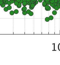
13 LIST OF FIGURES Figure 1.1 Fourier amplitudes developed from an example ground motion recording and SDOF oscillator response, illustrating the range of frequencies contributing to the response spectrum calculation....4 Figure 2.1 Figure 2.2 Number of earthquakes and recordings from the NGA-West2 EAS database used in the regression steps 1 and 3, versus frequency. The regressions were performed between Hz; higher frequencies are included in this figure only to display the rapid reduction of available data with increasing frequency....8 Magnitude versus rupture distance pairs of the NGA-W2 EAS database subset used in regression step 1, at 0.2, and 10.0 Hz....8 Figure 3.1 V s30 scaling of the linear site amplification terms, at f = 0.2, 0.5, 1, 5, 10, and 20 Hz Figure 3.2 Figure 3.3 Smoothing of the Hashash et al. [2018] coefficients f 3, f 4, and f 5, and the smoothing procedure of term f NL for example values of V s30 = 300 m/sec and I R = 0.8g...14 Data used to develop the I R EAS ref (f = 5 Hz) relationship, where I R is the peak ground acceleration on rock and EAS ref (f = 5 Hz) is the 5 Hz EAS on rock. Ground motions with I R > 0.01g are included, with symbols identifying M bins. I R is corrected to the reference site condition using the Abrahamson et al. [2014] linear site amplification model, and the EAS is corrected the reference V s30 condition using the linear site amplification model from this study Figure 4.1 Smoothing of source scaling (c 2 ) and near-source geometric spreading coefficients (c 4 ) Figure 4.2 Smoothing of the source scaling coefficient, c Figure 4.3 Smoothing of the source scaling coefficient, c n Figure 4.4 Smoothing of the source scaling coefficient c M Figure 4.5 Smoothing of the Z tor scaling coefficient, c Figure 4.6 Smoothing of the F NM style of faulting coefficient, c Figure 4.7 Smoothing of the linear V S30 scaling coefficient, c Figure 4.8 Smoothing of the Z 1 scaling coefficients, c

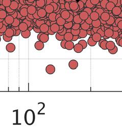
14 Figure 4.9 Smoothing of the anelastic attenuation coefficient, c Figure 4.10 Smoothing of the coefficient, c 1, and adjustment coefficient c 1a Figure 4.11 The geometric mean EAS spectra of the data used in the analysis, calculated using recordings from strike slip earthquakes with R RUP < 50 km, for M bins one unit wide, and adjusted to the reference V S30 condition Figure 5.1 Figure 5.2 Figure 5.3 Between-event residuals (B e ) versus M, Z tor, and F NM, and between site residuals (S2S s ) versus V s30, f = 0.2 Hz Between-event residuals (B e ) versus M, Z tor, and F NM, and between site residuals (S2S s ) versus V s30, f = 1 Hz Between-event residuals (B e ) versus M, Z tor, and F NM, and between site residuals (S2S s ) versus V s30, f = 5 Hz Figure 5.4 Within-site residuals (WS es ) versus M, R RUP, V s30, and Z 1 for f = 0.2 Hz Figure 5.5 Within-site residuals (WS es ) versus M, R RUP, V s30, and Z 1 for f =1 Hz Figure 5.6 Within-site residuals (WS es ) versus M, R RUP, V s30, and Z 1 for f = 5 Hz Figure 5.7 Within-site residuals (WS es ) versus R RUP, binned by M for f = 0.2 Hz Figure 5.8 Within-site residuals (WS es ) versus R RUP, binned by M for f = 1 Hz Figure 5.9 Within-site residuals (WS es ) versus R RUP, binned by M for f = 5 Hz Figure 5.10 Figure 5.11 Figure 5.12 Figure 5.13 Comparison of the model distance attenuation with the M 6.93 Loma Prieta data for (a) f = 0.5 Hz and (b) 5 Hz Comparison of the model distance attenuation with the M 7.2 El Mayor- Cucapah data for (a) f = 0.5 Hz and (b) 5 Hz Comparison of the model distance attenuation with the M 7.28 Landers data for (a) f = 0.5 Hz and (b) 5 Hz Comparison of the model distance attenuation with the M 6.69 Northridge data for (a) f = 0.5 Hz and (b) 5 Hz Figure 6.1 Median model spectra for a strike-slip scenario at R RUP = 30 km, Z tor = 0 km and with reference Vs 30 and Z 1 conditions (solid lines) compared with the additive double-corner frequency source spectral model with typical WUS parameters (dashed lines) Figure 6.2 Median model EAS spectra for a set of scenarios described by the parameters in each title....46

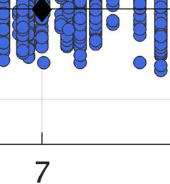
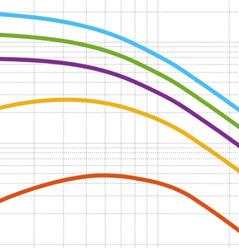
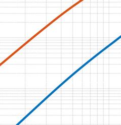
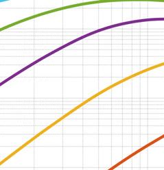
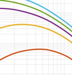
15 Figure 6.3 Figure 6.4 Figure 6.5 Figure 6.6 Figure 6.7 Figure 6.8 Figure 6.9 Distance scaling of the median EAS (solid lines) for a strike-slip scenario with reference Vs 30 and Z 1 conditions, for four frequencies. For reference, the distance scaling of the Chiou and Youngs [2014] model for PSA is shown for the same scenarios with the dash-dotted lines, where the PSA values have been scaled to the R RUP = 0.1 km EAS values M scaling of the median EAS for a strike slip surface rupturing scenario with reference Vs 30 and Z 1 conditions for f = 0.2, 1, 5, and 20 Hz M scaling of the median model for four distances, at f = 0.5 Hz for a strike slip earthquake rupturing the surface with reference Vs 30 and Z 1 conditions, compared with results from finite-fault simulations M scaling of the median model for four distances, at f = 1 Hz for a strikeslip earthquake rupturing the surface with reference Vs 30 and Z 1 conditions compared with results from finite-fault simulations M scaling of the median model for four distances, at f = 5 Hz for a strikeslip earthquake rupturing the surface with reference Vs 30 and Z 1 conditions, compared with results from finite-fault simulations (a) V s30 scaling of the median model for a M 7 strike slip earthquake rupturing the surface with reference Z 1 conditions at R RUP = 30 km. The solid lines represent the total (linear and nonlinear) V s30 scaling and the dashed lines represent only the linear portion of the V s30 scaling; (b) Z 1 scaling of the median model for the same scenario with V s30 = 300 m/sec; (c) scaling of the modified Hashash et al. [2018] nonlinear site term with M, for R RUP = 30 km and V s30 = 300 m/sec; and (d) scaling of the modified Hashash et al. [2018] nonlinear site term with R RUP, for M 7 and V s30 = 300 m/sec Standard deviation components calculated directly from the regression analysis for all magnitudes...53 Figure 6.10 Magnitude scaling of the standard deviation terms for f = 1 and 5 Hz Figure 6.11 Frequency dependence of the standard deviation model Figure 6.12 Figure 6.13 (a) Total standard deviation model for M 3, 5, and 7; and (b) median (solid lines) and median plus and minus one (dashed lines) EAS spectra for M 3, 5, and 7 scenarios Comparison of the standard deviation components between the Bora et al. [2015], Stafford [2017] models and this model, for a M 5 earthquake. Panels (a) through (d) show the comparison of, S2S, and SS, and, respectively....57

16

17 1 Introduction The traditional approach for developing ground-motion models (GMMs) for engineering applications is to use response spectral values for a range of spectral periods. The response spectra GMMs can be used in either deterministic or probabilistic seismic hazard analyses to develop design response spectra. The response spectral values represent the response of a simple structure to the input ground motion and does not directly represent the ground motion itself. As an alternative, Fourier spectral values can be used instead of response spectral values. There are several advantages to using Fourier spectra in place of response spectra: (1) the scaling of Fourier spectra in the GMM is easier to constrain using seismological theory, (2) linear site response remains linear at all frequencies and does not depend on the spectral content of the input motion, as is the case for response spectra [Bora et al. 2016], and (3) for calibrating input parameters and methods for finite-fault simulations based on comparisons with GMMs, Fourier spectra are more closely related to the physics in the simulations. An empirical Fourier spectrum GMM for shallow crustal earthquakes in California and Nevada based on the Pacific Earthquake Engineering Research Center (PEER) Next Generation Attenuation-West 2 (NGA-West2) database [Ancheta et al. 2014] is developed. The groundmotion parameter used in the GMM is the smoothed effective amplitude spectrum (EAS), as defined by PEER [Goulet et al. 2018]. The effective amplitude spectrum EAS is the orientationindependent horizontal component Fourier amplitude spectrum (FAS) of ground acceleration that can be used with random vibration theory to estimate the response spectral values. This paper describes the development of the empirical model using ground-motion data as the foundation, along with finite-fault simulations computed using the SCEC Broadband Platform [Maechling et al. 2015] to constrain the near-fault large-magnitude scaling, and the analytical site response modeling to capture the nonlinear site amplification [Hashash et al. 2018]. Rather than simply fitting the empirical data, emphasis is placed on building the model using both the empirical data and analytical results from these seismological and geotechnical models so that the GMM extrapolates in a reasonable manner. A MATLAB program that implements the EAS GMM is provided in an electronic appendix. A model for the interfrequency correlation of residuals derived from this GMM is presented in Bayless and Abrahamson [2018].

18 1.1 EFFECTIVE AMPLITUDE SPECTRUM GROUND-MOTION INTENSITY MEASURE The EAS, defined in Kottke et al. [2018] and used in the PEER NGA-East project [PEER 2015; Goulet et al. 2018], can be calculated from an orthogonal pair of FAS using Equation (1.1): EAS f FASHC1 f FASHC 2 f (1.1) 2 where FAS HC 1 and FAS HC 2 are the FAS of the two orthogonal horizontal components of the ground motion and f is the frequency in Hz. The EAS is independent of the orientation of the instrument. Using the average power of the two horizontal components leads to an amplitude spectrum that is compatible with the use of random vibration theory (RVT) to convert Fourier spectra to response spectra. The EAS is smoothed using the Konno and Ohmachi [1998] smoothing window, which has weights and window parameter defined by Equations (1.2) and (1.3): W f 2 b b w sin blog f f blog f fc c 4 The smoothing parameters are described in Kottke et al. [2018]: W is the weight defined at frequency f for a window centered at frequency f c and defined by the window parameter b. The window parameter b can be defined in terms of the bandwidth, in log 10 units, of the smoothing window, b w. The Konno and Ohmachi smoothing window was selected by PEER NGA-East because it led to minimal bias on the amplitudes of the smoothed EAS when compared to the unsmoothed EAS. The bandwidth of the smoothing window, b = , was selected such that the RVT calibration properties before and after smoothing were minimally affected [Kottke et al. 2018]. For consistency with the PEER database used to develop empirical FAS models, the smoothed EAS is used with the same smoothing parameters as described in Kottke et al. [2018]. (1.2) (1.3) 1.2 ON THE SELECTION OF FOURIER AMPLITUDES In seismic hazard and earthquake engineering applications, the pseudo-spectral acceleration (PSA) of a 5% damped single degree of freedom (SFOF) oscillator is a commonly used intensity measure (IM). The PSA is useful for many applications; however it has drawbacks which are discussed here. The EAS component of the FAS is used as the IM for this study, because the FAS is a more direct representation of the frequency content of the ground motions than PSA and is better understood by seismologists. This leads to several advantages, both in the empirical modeling and in forward application. The reasoning behind these claims is explained in this section. 2

19 The PSA calculation involves solving the differential equation for the response of a SDOF oscillator (with given damping) due to a specified forcing function, selecting the peak response of the oscillator, and scaling the peak oscillator displacement by the square of the oscillator natural frequency,. This calculation can be repeated for a range of oscillators with different natural frequencies to develop a response spectrum. The elastic SDOF oscillator response is described by the following second order, linear, inhomogeneous differential equation: ma t cv t ku t p t (1.4) where m is the SDOF lumped mass, a(t) denotes the SDOF lateral acceleration, c denotes the viscous damping coefficient, v(t) denotes the SDOF lateral velocity, k denotes the lateral stiffness, u(t) denotes the SDOF lateral displacement relative to the ground, and p(t) denotes the time-dependent forcing function due to the earthquake ground motion [Chopra 2007]. Duhamel s convolution integral, also known as the unit impulse response procedure, is one approach to solving a linear differential equation, such as the one given by Equation (1.4). With this method, the response of the system (initially at rest) to a unit impulse force is shown (e.g., in Chopra [2007] to be: 1 t ht e sin d t, t m (1.5) d where is the time instance of the impulse, d is the damped natural frequency, and is the fraction of critical damping. The entire loading history (such as that due to ground acceleration) can then be represented as a succession of infinitesimally short impulses, each producing its own response of the form of Equation (1.5). Since the system is linearly elastic, the total response is the superposition of the responses to all impulses which make up the entire loading history. Taking the limit of the sum as the width of the impulse approaches zero leads to the general expression of Duhamel s integral for an arbitrary forcing function: 1 t u t p e t d p h t h t p t m 0 0 d t t sin d (1.6) where is the convolution operator. Equation (1.6) is called the convolution integral because convolution is performed in the time domain between the unit impulse response (h), and the force due to ground acceleration (p). Then, by the convolution property of the Fourier transform, the time-domain convolution of h and p can be expressed in the frequency domain as the pointwise multiplication of the Fourier transforms of h and p. In Figure 1.1, these steps are shown using an example recorded acceleration time history. In the figure, the thin solid black line is the FAS of the recorded acceleration time history, or F p, where F denotes the Fourier transform operator. The solid heavy lines are the FAS of F h. F h is plotted for three different oscillator the SDOF oscillator impulse response, or frequencies: 0.5, 2.0, and 10.0 Hz, as identified in the figure legend. The dashed lines are the 3

20 FAS of the SDOF response to the ground motion, Equation 1.4, and the convolution property of the Fourier transform, for a given oscillator frequency, F u Fp F h. This result can be confirmed qualitatively in Figure 1.1. Figure 1.1 illustrates thatt oscillators with different natural frequencies are controlled by different frequency ranges of the ground motion. At relatively higher oscillator frequencies (e.g., 10 Hz; green lines in Figure 1.1), where there is little energy left to resonate the oscillator, the PSA ordinates are dominated by a wide frequency band of the ground motion that ultimately equals the integration over the entire spectrum of the input ground motion [Bora at al. 2016]. This can be observed in Figure 1.1, where the dashed green line traces the ground motion FAS for frequencies less than about 4 Hz. The short period PSA is then controlled by the dominant period of the input ground motion, rather than the natural period of the oscillator. F u, at the same threee frequencies. By Figure 1.1 Fourier amplitudes developed from ann example ground motion recording and SDOF oscillator response, illustrating the range of frequencies contributing to the response spectrum calculation. 4

21 In summary, PSA provides the spectrum of peak response from a SDOF system, which is influenced by a range of frequencies, and the breadth of that range is dependent on the oscillator period. The FAS provides a more direct representation of the frequency content of the ground motions, and since the Fourier transform is a linear operation, the FAS is a much more straightforward representation of the ground motion. As a result, recordings from small earthquakes can be used to constrain path and site effects without dependence on response spectral shape. Numerous seismological models of the FAS are available (e.g. Brune [1970] and Boore et al. [2014]) to provide a frame of reference during model development. Additionally, using FAS more easily facilitates future calibration of the inter-frequency correlation of groundmotion simulation methods because there is not a strong reversal of the correlation coefficients at high frequencies, as described in Bayless and Abrahamson [2018]. 5

22 6

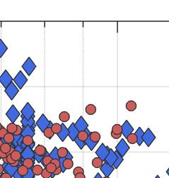
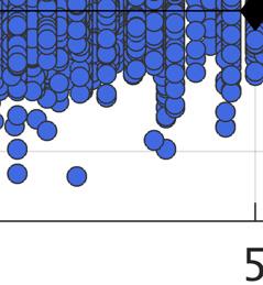
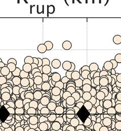
23 2 Ground-Motion Data The PEER NGA-West2 strong-motion database includes over 21,000 three-component strongmotion records recorded worldwide from shallow crustal earthquakes, including aftershocks, in active tectonic regimes since 2003 [Ancheta et al. 2014]. Earthquake magnitudes in the full database range from 3 to 7.9 and rupture distances extend to over 1500 km. Earthquakes and recordings identified as questionable in quality or with undesirable properties are excluded; see Abrahamson et al. [2014] for a complete list of criteria for exclusions. At distances under 100 km, recordings from crustal earthquakes worldwide are retained to constrain the magnitude scaling and geometric spreading. At the larger distances (up to 300 km), region-specific anelastic attenuation and linear site effects due to the regional crustal structure are accounted for by including recordings only from California and Nevada. Only events with at least five recordings per earthquake are included. The EAS has been calculated for each record in the database up to the Nyquist frequency by PEER [Kishida et al. 2016]. The usable frequency range limitations of each record are accounted for by applying the recommended lowest and highest usable frequencies for response spectra determined from Abrahamson and Silva [1997] as: Lowest usable frequency (LUF) 1.25 max HPF, HPF (2.1) HC1 HC 2 1 Highest usable frequency (HUF) min LPF HC1, LPFHC 2 (2.2) 1.25 where HPF is the record high-pass filter frequency, LPF is the record low-pass filter frequency, and HC1 and HC2 are the two horizontal components of a three-component time series. The factors of 1.25 in Equations (2.1) and (2.2) were originally used by Abrahamson and Silva [1997] to ensure that the filters did not have a significant effect on the response spectral values. By limiting the usable period range using these factors, the frequency interval of the impulse response of a 5% damped oscillator will not exceed the filter values. And retaining this usable frequency range maintains consistency with the response spectrum calculations. Based on inspection of the usable frequency range of the data, the LUF was restricted to a minimum value of 0.1 Hz, and the HUF was restricted to a maximum value of 24 Hz for all recordings. Therefore, the regressions were performed between Hz. After screening for record quality, recording distance, minimum station requirements, and frequency limitations, the final dataset consists of 13,346 unique records from 232 7

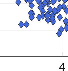
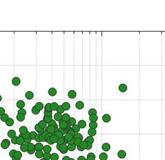
24 earthquakes, both of which vary as a function of frequency. Figure 2.1 shows the frequency dependence of the number of earthquakes and recordingss used in regressions steps 1 and 3 ( listed in Table 4.2 and explained in Section 4). Figure 2.2 shows a magnitude versuss rupture distance scatterplot of the NGA-West2 database subsets used in regression step 1 at f = 0..2 and 10 Hz. Figure 2.1 Number of earthquakes and recordings from the NGA-West2 EAS database used in the regression stepss 1 and 3, versus frequency. The egressions were performed between Hz; higher frequencies are included in this figure only to display the rapid reduction of available dataa with increasing frequency. Figure 2.2 Magnitude versus rupture distance pairs of the NGA-W2 EAS database subset used in regression step 1, at 0.2, and 10.0 Hz. 8

25 3 Median Model Functional Form The model parameters are defined in Table 3.1. The scaling of the source is primarily described by moment magnitude (M). Source effects are also modeled using the depth to the top of the rupture plane (Z tor ), and a style-of-faulting flag for normal faults (F NML ). These source effects can be considered as proxies for stress drop scaling. The closest distance to the rupture plane, R RUP is used as the distance measure for path scaling. The linear and nonlinear site effects are parameterized using V s30, the time-averaged shear-wave velocity in the top 30 m of the soil column below the site. Use of V s30 does not imply that 30 m is the key depth range for the site response, but rather that V s30 is correlated with the entire soil profile [Abrahamson and Silva 2008]. The scaling with respect to soil depth is parameterized by the depth to the shear-wave velocity horizon of 1 km/sec, Z 1. Table 3.1 Model parameter definitions. Parameter EAS M Z tor F NM R RUP V s30 Z 1 I r Definition Effective amplitude spectrum (g-sec). The EAS is the orientation-independent horizontal component Fourier amplitude spectrum (FAS) of ground acceleration, defined in Goulet et al. [2018]. Moment magnitude Depth from the surface to the top of the rupture plane (km) Style of faulting flag; 1 for Normal faulting earthquakes, 0 for all others. Rupture distance (km) Time averaged shear wave velocity in the upper 30 meters (m/sec) Depth from the surface to shear wave velocity horizon of at least 1 km/sec (km) Peak ground acceleration for the Vs30 = 760 m/sec condition (g) 9

26 The model prediction for the EAS (units g-sec) ground motion is given by Equation (3.1): ln EAS = ln EASmed (3.1) where is the total aleatory variability, and the standard-normal random variable is the number of standard deviations above or below the median. The median estimate of the EAS (EAS med, with units g-sec) can be calculated from Equation (3.2), where each of the model components are described in the following sections. ln EASmed f f f f f f (3.2) M P S Ztor NM Z1 3.1 MAGNITUDE SCALING, f M To capture the effects of energy radiated at the source, the formulation of the magnitude scaling is adopted from the Chiou and Youngs [2008; 2014] GMMs for response spectra. A polynomial magnitude scaling formulation was tested (e.g., Abrahamson et al. [2014]), and after evaluating the data found that both formulations fit the data well, but the Chiou and Youngs [2014] formulation would extrapolate more reasonably. Additionally, the Chiou and Youngs [2014] formulation has undergone several years of testing and refinement and is based on seismological models for the source FAS [Chiou and Youngs 2008], which translates directly to this application. The expression for the magnitude scaling is given by Equation (3.3): cn cm M f c c M 6 c ln 1e (3.3) M The components of f M are described in Chiou and Youngs [2008]. To recap, the formulation captures approximately linear magnitude scaling at low frequencies (well below the source corner) and high frequencies (well above the source corner) with a nonlinear transition in between, where the transition shifts to lower frequencies for larger magnitudes. The coefficient c 1 works jointly with the c 2 and c 3 terms to approximately represent the mean spectral shape after correcting for all other adjustments. The coefficient c 2 is the frequency independent linear M scaling slope for frequencies well above the theoretical corner frequency. The term with coefficient c 3 captures both the approximately linear scaling of the FAS below the theoretical corner frequency, and the non-linear transition to that scaling. The coefficient c n controls the width of the magnitude range over which the transition between low- and high-frequency linear scaling occurs, and the coefficient c M is the magnitude at the midpoint of this transition. All of the magnitude scaling terms were determined in the regression. 3.2 PATH SCALING, f P Together with the magnitude scaling, the extensively-tested path scaling formulation of Chiou and Youngs [2014] is utilized: ˆ hm fp c4ln RRUP c5cosh c6max M c, c4 ln R c7rrup (3.4) 10

27 R ˆ R 50 (3.5) 2 2 RUP The components of Equation (3.4) are described in Chiou and Youngs [2008]. To recap, the term with coefficient c 4 captures near-source geometric spreading, which is magnitude and frequency dependent. The magnitude and frequency dependence on the geometric spreading is introduced by adding a term to the rupture distance inside the log-distance term, expressed by the term with coefficient c 5. This additive distance is designed to capture the near-source amplitude saturation effects of the finite-fault rupture dimension. This term is a frequency-dependent constant for small magnitudes, and transitions to be proportional to exp (M) for large magnitudes, with the largest additive distance at high frequencies. Since the hyperbolic cosine is a monotonically increasing function, the coefficient c 5 controls the scaling of this term, and coefficients c 6 and c hm control the gradient. Since the coefficients c 5, c 6, and c hm are multiplied with c 4, there is potential for trade-off between them. The regression procedure is started with the values for coefficients c 5, c 6, and chm from Chiou and Youngs [2014] to obtain c 4 from the data, ensuring the model did not oversaturate. Using Equations (3.3) and (3.4), the full saturation condition (no magnitude scaling at zero distance) leads to the following constraint on the coefficients: c 2 = c 4 c 6. For c 2 values larger than the full saturation value, there will be a positive magnitude scaling at zero distance (i.e., not full saturation). It is reasonable for the EAS to have some scaling at zero distance even though the PSA is nearly fully saturated at high frequencies. The PSA saturates in part because the procedure involves selecting the peak response of the oscillator over all time, meaning it is not affected by duration. Conversely, the EAS is not a peak response operator, and so it will continue to scale for large magnitudes at short distance due to the longer source durations. This is the contribution of the lower amplitudes over the duration of the signal. The near-source saturation of magnitude scaling is checked against the data and against finite fault simulations (see Section 6 for more details) and the EAS saturation in this model does not disagree with those from the simulations. In later stages of the regression, the coefficients c 5, c 6, and c hm are also determined empirically. The values from the regression do not change enough to impact the model, so coefficient values are fixed from Chiou and Youngs [2014] for c 5, c 6, and c hm in the final model. Thus, the coefficients c 2 and c 4 control the saturation in the model development. Following Chiou and Youngs [2014], at large distances, the distance scaling smoothly transitions to be proportional to R -0.5 to model surface wave rather than body wave geometric ln R ˆ term, which controls at distances spreading effects. This effect is introduced with the greater than 50 km by subtracting the c 4 coefficient and imposing a -0.5 slope. Effects of crustal anelastic attenuation (Q) are captured through the term with the frequency-dependent coefficient c 7. The Q scaling does not require magnitude dependence for the EAS. 11

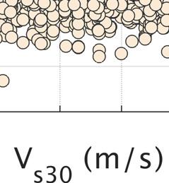
28 3.3 SITE RESPONSE, f S The V S30 (m/sec) dependence of site amplification is modeled using Equation (3.6): fs fsl fnl (3.6a) f f s30 SL c8 ln f min V,1000 I ln f 1000 R 3 NL 2 f3 2 4 s f5min V 30, Vref 360 f5 Vref 360 (3.6b) (3.6c) f f e e (3.6d) IR ref f ln ln EAS 5 Hz (3.6e) where the linear site amplification is given by f SL, and the nonlinear site amplification is given by f NL, which is the analytical site amplification function for FAS in the western United States (WUS) modified from Hashash et al. [2018]. The linear site term, f SL, is formulated as a linear function of ln(v s30 ) and is centered on the reference V s30 of 1000 m/sec. The f SL term is determined in the regression analysis. Abrahamson et al. [2014] observed that at long periods, the scaling of PSA with V s30 became weaker for higher V s30 values, and, therefore, selected a model that does not scale with V s30 above some maximum value, V 1 = 1000 m/sec. Inclusion of this feature is based on evaluation of the data (Figure 3.1), which implies that above 1000 m/sec, the correlation between V s30 and the deeper profile no longer holds. Below 1000 m/sec, the linear site amplification terms approximately scales linearly with ln(v s30 ), so the regional linear V s30 -based site amplification is modeled with a single frequency-dependent coefficient, c 8. The nonlinear site amplification, f NL, is constrained using a purely analytical model rather than obtaining it from the data. Empirical evaluations of the nonlinear effects are limited by the relatively sparse sampling of ground motions expected to be in the nonlinear range in the NGA- West2 database [Kamai et al. 2014]. Therefore, the Hashash et al. [2018] nonlinear site amplification term, f NL, was adopted to model nonlinear soil amplification. This model was developed analytically by performing large-scale 1D site response simulations of input rock motions propagated through soil columns representative of WUS site conditions. Hashash et al. (2018) produced linear and nonlinear site amplification models for the PSA and FAS. Equations (3.6c) and (3.6d) are the nonlinear FAS amplification components of the Hashash et al. [2018] model developed for the WUS. In these equations, f 3, f 4, and f 5 are frequency-dependent coefficients, I R is the peak ground acceleration (PGA, in units g) at rock outcrop, and V ref is the limiting velocity beyond which there is no amplification relative to the reference rock condition, set to 760 m/sec [Hashash et al. 2018]. In this model, almost no nonlinearity is applied at frequencies below 1.0 Hz and the modification approaches zero for small values of the input motion (I R ) and as V s30 approaches V ref. 12

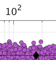
29 Figure 3.1 V s30 scaling of the linear site amplification terms, at f = 0.2, 0.5, 1, 5, 10, and 20 Hz. To ensure smooth spectra in the GMM, a smoothed version of the Hashash et al. [2018] nonlinear site amplification model is implemented. The smoothing of coefficients f 3, f 4, and f 5 in frequency space are shown in Figure 3.2. The maximumm frequency of the Hashash et al. [2018] model is 13.3 Hz, and the coefficients of the model reduce the nonlinear effect to zero for frequencies greater than this value simply due to the lack of FAS values at higher frequencies. Physically, this is not realistic behavior. To include nonlinear effects at the higher frequencies, the Hashash et al. [2018] model is modified by taking the minimum value of f NL over all frequencies and constrain all higher frequencies to take the same value. An example of this method (for input values of V s30 = 300 m/sec and I R = 0.8g) is shown in Figure 3.2. To utilize the Hashash et al. [2018] nonlinear model requiress the PGA on rock. Since the model is for the EAS, an estimate of the PGA (in units g) for the reference-site at f = 5 Hz (in units g-sec), condition is developed as a function of the EAS for the reference site conditionn 13

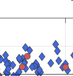
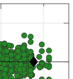
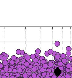
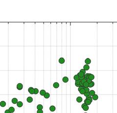
30 given by Equation (3.6e). The EAS at f = 5 Hz is used to estimate PGA because this is approximately the predominant frequency of the ground motions and should correlate strongly with the PGA. In Figure 3.3, the data used to develop the I R EAS ref (f = 5 Hz) relationship are shown. Ground motions with I R > 0.01g are included, with symbolss identifying data within unit M bins. In Figure 3. 3, I R is corrected to the reference site condition using the Abrahamson et al. [2014] linear site amplification model, and the EAS is corrected the reference V s30 condition using the linear site amplification model from this study. The least squares fit given by Equation (3.6e) is shown with the dashed line. Different M and distance ranges were evaluated similarly, with minimal differences in the slope of the relationship.. Figure 3.2 Smoothing of the Hashash et al. [2018] coefficients f 3, f 4, and f 5, and the smoothing procedure of term f NL for example values of V s30 = 300 m/sec and I R = 0.8gg 14

31 Figure 3.3 Data used to develop the I R EAS re ef(f = 5 Hz) relationship, where I R is the peak ground acceleration onn rock and EAS ref (f = 5 Hz) is the 5 Hz EAS on rock. Ground motions with I R > 0.01g are included, with symbols identifying M bins. I R is corrected to the referencee site condition using the Abrahamson et al. [2014] linear site amplification model, and the EAS is corrected the reference V s30 condition using the linear site amplification model from this study. 3.4 DEPTH TO TOP OF RUPTURE SCALING, f To model differences in the ground motions for surface and buried ruptures, the depth to the top of rupture scaling model takes the form of Equation (3.7): f Z tor c9 m Ztor min, 20 f Ztor where c 9 c is frequency dependent, and Z tor is non-negative and measured in km. The Z tor scaling is capped at 20 km to prevent unbounded scaling with Z to or. (3.7) 15

32 3.5 NORMAL STYLE OF FAULTING EFFECTS, f NM To model the differences in ground motions for normal style faults, the normal faulting term is: f NM c F (3.8) 10 NM where F NM is 1 for normal style faults and 0 for all others, and c 10 is determined in the regression. A style of faulting term for reverse events was considered but not included, because this term was highly correlated with Z tor. Therefore, the reverse style of faulting scaling is captured in f Z tor. 3.6 SOIL DEPTH SCALING, f Z1 To model the scaling with respect to sediment thickness, the Abrahamson et al. [2014] formulation is adopted, which is parameterized by the depth to shear wave velocity horizon of 1.0 km/sec, Z 1 (units of km). This model takes the form: where Z1 ref f c Z1 11 min Z, 2.0 0, 01 1 c11 ln Z ref c c c c for Vs 200 m / sec for 200 Vs 300 m / sec for 300 Vs 500 m / sec for V 500 m / sec 11a 30 11b 30 11c 30 11d s30 (3.9a) (3.9b) V exp ln s Z ref 4 4 (3.9c) is the reference Z 1 for the regional model for California and Nevada. Equation (3.9c) was developed by Chiou and Youngs [2014] to account for regional differences in the V s30 Z 1 relationships in the data. Abrahamson et al. [2014] showed that the Z 1 scaling is dependent on the V s30 value and used the V s30 bins in Equation (3.9b) to model this dependence; the same bins are used here. The soil depth scaling is capped to Z 1 = 2 km based on the range of the data and to avoid unconstrained extrapolation. 16

33 4 Regression Analysis The random-effects model is used for the regression analysis following the procedure described by Abrahamson and Youngs [1992]. This procedure leads to the separation of total residuals into between-event residuals ( B) and within-event residuals ( W), following the notation of Al Atik et al. [2010]. For large numbers of recordings per earthquake, the between-event residual is approximately the average difference in logarithmic-space between the observed IM from a specific earthquake and the IM predicted by the GMM. The within-event residual ( W) is the difference between the IM at a specific site for a given earthquake and the median IM predicted by the GMM plus B. By accounting for repeatable site effects, W can further be partitioned into a site-to-site residual ( S2S) and the single-station within-event residual ( WS, also called the within site residual) (e.g., Villani and Abrahamson, 2015). Using this notation, the residuals take the following form: Y g X, B S2S WS (4.1) es e s es total Y g X, B S2S WS Y g X, B S2S WS total S2S SS es e s es es e s es where Y is the natural log of the recorded ground motion IM, g(x es, ) is the median GMM, X es is the vector of explanatory seismological parameters (magnitude, distance, site conditions, etc.), is the vector of GMM coefficients, and total is the total residual for earthquake e and site s. The residual components B, S2S, and WS are well-represented as zero-mean, independent, normally distributed random variables with standard deviations, S2S, and SS, respectively [Al Atik et al. 2010]. The total standard deviation,, is expressed as: S2S SS (4.2) (4.3) The regression is performed in a series of steps to prevent trade-off of correlated model coefficients and to constrain different components of the model using the data relevant to each piece. These steps are given in Table 4.1, along with the data used and parameters determined from each step. In Step 1-a, a dataset consisting of larger magnitudes and shorter distances is used to constrain the large magnitude scaling and near-source finite fault saturation, using data from all regions. In Steps 1-b through 1-d, the same data set is used, and the remaining source 17

34 effects are determined. In Step 2, the regionalized linear site amplification parameters are determined using the data from California and Nevada at distances within 100 km. In Steps 3-a through 3-c, data from California and Nevada are included out to 300 km distance. In these regression steps, the regional soil depth scaling, anelastic attenuation, and mean spectral shape coefficients are determined. For all steps the regression is performed independently at each of 239 log-spaced frequencies spanning Hz. Table 4.1 Regression steps. Step Data used Parameters free in the regression Parameters smoothed after the regression 1-a M > 4, R RUP 100 km, all regions c 1, c 2, c 3, c n, c M, c 4, c 7, c 8, c 9, c 10, c 11 1-b Same as 1-a c 1, c 3, c n, c M, c 7, c 8, c 9, c 10, c 11 1-c Same as 1-a c 1, c 5, c 6, c hm, c 7, c 8, c 9, c 10, c 11 1-d Same as 1-a c 1, c 7, c 8, c 9, c 10, c 11 1-e Same as 1-a c 1, c 7, c 8, c 10, c 11 2 M > 4, R RUP 100 km, from CA/Nevada c 1, c 7, c 8, c 11 3-a M > 3, R RUP 300 km, from CA/Nevada c 1, c 7, c 11 3-b Same as 3-a c 1, c 7 c 2, c 4 (M, path) c 3, c n, c M (M) c 5, c 6, c hm (path) c 9 (Z tor ) c 10 (F NM ) c 8 (V S30 ) c 11 (Z 1 ) c (Q) 3-c Same as 3-a c 1 c SMOOTHING The model coefficients are smoothed in a series of steps as outlined in Table 4.1. Smoothing of the coefficients is performed to assure smooth spectra and, in some cases, to constrain the model to a more physical behavior where the data are sparse [Abrahamson et al. 2014]. Tables of the values of the final smoothed coefficients are available in Electronic Appendix B. Figure 4.1 through Figure 4.10 show the regressed model coefficients plotted versus frequency, before and after smoothing. The coefficients c 2 and c 4 are frequency independent and are determined from regressions in the high frequency range. The coefficients c 3, c n, and c M require only minor smoothing to assure smooth spectra in the final model, including extrapolation outside the ranges well constrained by data. The smoothing of c 7 (the anelastic attenuation term) is constrained to be non-positive at all frequencies so that the model does not 18

35 unintentionally increase in amplitude at very large distances. Minimal smoothing is required for the coefficient c 8 (the linear V S30 term). The coefficient c 9 (the Z tor term) takes on negative values at low frequencies implying small de-amplification of low frequency ground motions with increasing Z tor. The data lead to a large drop in c 10 (the normal faulting term) at low frequencies, but this is not included in the model because the theoretical basis is not clear; instead a frequency-independent constant is used (uniform scaling across frequencies) for normal style-offaulting earthquakes. The c 11 terms are smoothed as shown in Figure 4.8, where the uncertainty is largest for c 11a, which corresponds to the lowest V S30 bin with relatively fewer data. The c 1 coefficient works collectively with the c 3 term to represent the mean spectral shape after correcting for all other adjustments. In the regression, unexpected behavior of c 1 at low frequencies is observed, as shown in Figure At frequencies below about 0.3 Hz, the regressed coefficient values are equal to or larger than the 0.3 Hz value. If unmodified and combined with the c 3 term, this would lead to an irregular spectral bump at f < 0.3 Hz. Following Aki [1967], the mean spectrum should be approximately linear with a slope = 2 in this frequency range. Therefore, the c 1 coefficient is modified at low frequencies by constraining the slope from f 1.0 Hz down to 0.1 Hz, as shown in Figure The difference between the regressed values of c 1 and the constrained values of c 1 is denoted c 1a ; this adjustment coefficient is plotted in the lower portion of Figure By introducing the c 1a term, the model predicts smooth, theoretically appropriate spectra at low frequencies. This also allows for residuals which are zero-centered, which is required for computing the correlations of the residuals between frequencies. To account for this modification, the c 1a term must be added to the total standard deviation using Equation (2.21). The standard deviation model is discussed further below. This unexpected behavior of c 1 may be due to bias in the data. At low frequencies, the signal to noise ratio is commonly low [Douglas and Boore 2011]. This contributes to the drop off in data at low frequencies shown in Figure 2.1. Additionally, at low frequencies, the large epsilon (above average) ground motions are more likely to be above the signal to noise ratio, and therefore, be included in the database. Likewise, the below average ground motions are more likely to be below this ratio and be excluded. The net effect may be that, for the FAS at low frequencies, the database is biased towards higher ground motions. Observing the data, the mean spectra for certain binned magnitude and distance ranges contain this feature. As an example, Figure 4.11 shows the geometric mean spectra of a subset of the data used in the analysis. This figure is created using recordings from strike-slip earthquakes with R RUP < 50 km, for M bins one unit wide, and adjusted to the reference V S30 condition. Below about 0.3 Hz, the bump in the spectral shape in the data that causes the increase of c 1 is evident, especially for the data with M > 7 and M < 5. Other physical explanations of the cause of the increase in coefficient c 1 are not apparent. To check that long period basin effects are not the cause, the mean spectra are examined in the same way, but only including records with Z 1 < 0.15 km, and the same behavior is observed. To further test if basin effects are not adequately captured by the model, c 1 is fixed to the constrained shape and the residuals are mapped. We do not see regional or spatial trends in the mapped residuals, implying that basin effects are not the culprit. Understanding the physical cause of the long-period shape of the spectrum will be evaluated further in a future study. 19

36 Figure 4.1 Smoothing of source scaling (c 2 ) and near-sourcee geometric spreading coefficients (cc 4 ). Figure 4.2 Smoothing of the sourcee scaling coefficient, c 3. 20

37 Figure 4.3 Smoothing of the sourcee scaling coefficient, c n. Figure 4.4 Smoothing of the sourcee scaling coefficient c M. 21

38 Figure 4.5 Smoothing of the Z tor scaling coefficient, c 9. Figure 4.6 Smoothing of the F NM style of faulting coefficient, c

39 Figure 4.7 Smoothing of the linear V S30 scaling coefficient, c 8 8. Figure 4.8 Smoothing of the Z 1 scaling coefficients, c

40 Figure 4.9 Smoothing of the anelastic attenuation coefficient, c 7. 24

41 Figure 4.10 Smoothing of the coefficient, c 1, and adjustment coefficient c 1a. 25

42 Figure 4.11 The geometric mean EAS spectra of the data used in the analysis, calculated using recordings from strike slip earthquakes with R RUP < 50 km, for M bins one unit wide, and adjustedd to the reference V S30 condition. 4.2 EXTRAPOL LATION TO 100 HZ Model coefficients are obtained by regression for frequencies up to 24 Hz. At high frequencies, the FAS decays rapidly [Hanks 1982; Anderson and Hough 1984]. Anderson and Hough [1984] introduced the spectral decay factor kappaa () to model the rate of the decrease, where the amplitude of the log(fas) decays linearly versus frequency (linearr spaced), and is related to the slope. The total site amplification is the combined effect of crustal amplification and damping ( and Q), but the effect of is so strong that it controls the spectral decay of the FAS at high frequencies and is the only parameter specified in the extrapolation. The model is extrapolated using Equations (4.4): 26

43 D(, f) exp f (4.4a) V 30 ln 0.4 ln s f fmax fmax D f fmax (4.4b) EAS EAS, (4.4c) where D(, f ) is the Anderson and Hough [1984] diminution operator, and f max is the frequency beyond which the extrapolation occurs; f max = 24 Hz. The parameter is estimated from κ is estimated from V S30 using the relationship given by Equation (4.4b). This relationship is selected based on the range of 0 V S30 correlation models presented in Figure 2 of Ktenidou et al. [2014]. The scatter observed in these correlations is large, as described in Ktenidou et al. [2014]. 27

44 28

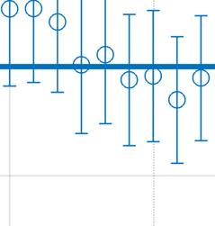
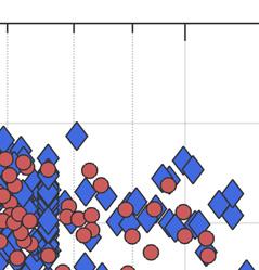
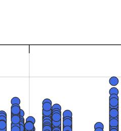
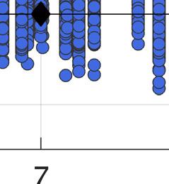
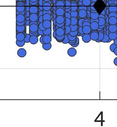
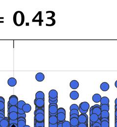
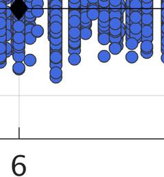
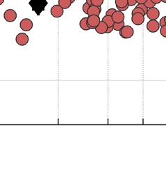
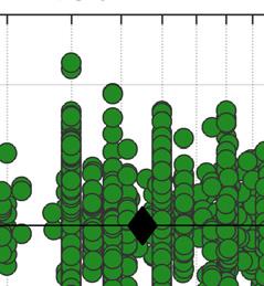
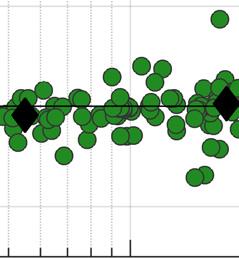
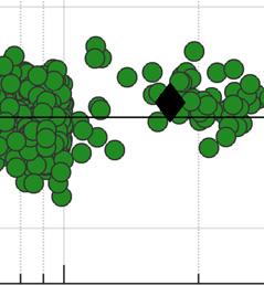
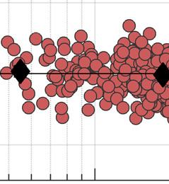
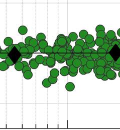
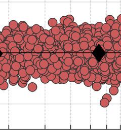
45 5 Residuals The model is evaluated by checking the residuals from the regression analysis as functions of the main model parameters. Example figures are included below, and a larger set of residual figures are available in Electronic Appendix A. 5.1 BETWEEN-EVENT AND BETWEEN-SITE RESIDUALS Examples of the dependence on the source parameters of the between-event residuals at f = 0.2, 1.0, and 5.0 Hz are given in Figure 5.1 through Figure 5.3. In these figures, the diamond-shaped markers represent events from California and Nevada, and circles represent events from all other regions. There is not a strong magnitude dependence of the B. For Z tor, there is no trend in the residuals at high frequencies, where the model increases the ground motion with increasing Z tor. There is a potential difference in Z tor scaling between regions at low to moderate frequencies, an effect which should be evaluated further in the future. For F NM, there is also no trend in the residuals at high frequencies, but at the lower frequencies, potential regional differences exist. The normal faulting term is constrained by sparse data (only 10 events at 0.2 Hz, including six from Italy), so this term is not refined further. Figure 5.1 through Figure 5.3 also show the dependence of the between-site residuals on V S30. Overall, there is no trend in S2S versus V S30. The standard deviation of these residuals ( S2S ) is comparable to at frequencies greater than about 2 Hz. The standard deviations are discussed further in Section

46 Figure 5.1 Between-even nt residuals (B e ) versus M, Z tor, and F NM, and between site residuals (S2S s ) versus V s30, f = 0.2 Hz. 30

47 Figure 5.2 Between-even nt residuals (B e ) versus M, Z tor, and F NM, and between site residuals (S2S s ) versus V s30, f = 1 Hz.. 31

48 Figure 5.3 Between-even nt residuals (B e ) versus M, Z tor, and F NM, and between site residuals (S2S s ) versus V s30, f = 5 Hz.. 32

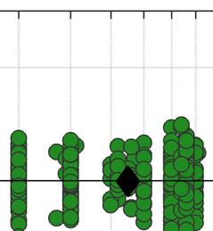
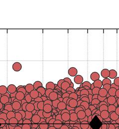
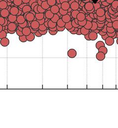
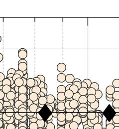
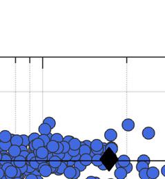
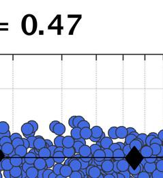
49 5.2 WITHIN-SITE RESIDUALS Examples of the dependence on the model parameters of the within-site residuals at f = 0.2, 1.0, and 5.0 Hz are given in Figure 5.4 through Figure 5.6. The filled circles are individual residuals, and the black diamonds with whiskers represent the mean and 95% confidence interval of the mean for binned ranges of the model parameter. Overall, there is no trend observed in WS versus moment magnitude. The linear site response model is evaluated through the V S30 and Z 1 dependence of the residuals. Overall, no strong trends are observed against V S30, except for the highest V S30 values at low frequencies, where the residuals are slightly positive, indicating model under-prediction. The data are very sparse in this range (six records with V S30 > 1500 m/sec and 106 records with V S30 >1200 m/sec. No strong Z 1 dependencies on the residuals are observed. The distance scaling of the model is evaluated using the distance-dependence of WS as shown in Figure 5.4 through Figure 5.6. Additionally, the distance dependence is evaluated using magnitude binned residuals. Examples of the distance dependence binned by magnitude are shown in Figure 5.7 through Figure 5.9, where the magnitude bin ranges are given in the figure legends. In the distance range of about km, there are no strong trends or biases of the residuals. At low frequencies, for distances beyond 100 km and in the M bin, the WS residuals are biased positive. This is likely due to the relatively limited data within this bin, and that the model scaling is appropriate even though these particular residuals are not zero-centered. Thus, neither the magnitude nor distance scaling are adjusted to center these residuals. At distances shorter than 1 km and for frequencies greater than about 2 Hz, there is a small systematic negative bias in the residuals (Figure 5.6). This means the near-fault saturation in this model is not as strong as indicated by the data. Graizer [2018] chose to incorporate oversaturation (a peak in the distance scaling at about 5 km) into his ground motion models. The oversaturation of distance scaling is intentionally avoided in this model. Because the available ground-motion data is extremely sparse at such close distances, this model is compared with the saturation from finite fault earthquake simulations (see Model Summary section of this paper for more details). Based on these results, and on the sparsity of the data, the small bias in the shortdistance residuals is accepted. The distance dependence of the model is also compared with data from four wellrecorded WUS earthquakes in Figure 5.10 through Figure 5.13: the 1989 M 6.9 Loma Prieta, 2010 M 7.2 El Mayor-Cucapah, 1992 M 7.3 Landers, and 1994 M 6.7 Northridge. In these figures, the top panels compare the recorded EAS with the model-predicted EAS at each site, including the event term for that earthquake. The lower panels show the within-event residuals for the same sites versus R RUP. Residuals for El Mayor-Cucapah, the most well-recorded large earthquake in California, show no bias or trend at either frequency. Besides a few outliers, the remaining three events have attenuation which does not disagree with the median model and is captured on average. 33

50 Figure 5.4 Within-site residuals ( WS Ses) versus M, RRUP, Vs30, and Z1 for f = 0.2 Hz. 34

51 Figure F 5.5 Within-site e residuals ( WSes) versu us M, RRUP, Vs30, and Z1 fo or f =1 Hz. 35

52 Figure 5.6 Within-site residuals ( WS Ses) versus M, RRUP, Vs s30, and Z1 for f = 5 Hz. 36

53 Figure 5.7 Within-site residuals WS ( es ) versus R RUP, binned by M for f = 0.2 Hz. 37

54 Figure 5.8 Within-site residuals (WS es ) versus R RUP, binned by M for f = 1 Hz. 38

55 Figure 5.9 Within-site residuals (WS es ) versus R RUP, binned by M for f = 5 Hz. 39

56 Figure 5.10 Comparison of the model distancee attenuationn with the M 6.93 Loma Prieta dataa for (a) f = 0..5 Hz and (b)) 5 Hz. (a) (b) Figure 5.11 Comparison of the model distancee attenuationn with the M 7.2 El Mayor-Cucapah data for (a) f = 0.5 Hz and (b) 5 Hz. 40

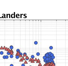
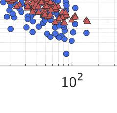
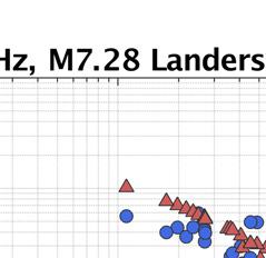
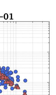
57 (a) (b) Figure 5.12 Comparison of the model distancee attenuationn with the M 7.28 Landers data for (a) f = 0.5 Hz and (b) 5 Hz. (a) (b) Figure 5.13 Comparison of the model distancee attenuationn with the M 6.69 Northridge data for (a) f = 0.5 Hz and (b) 5 Hz. 41

58 42

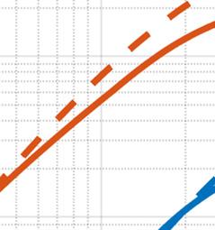
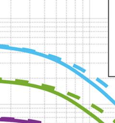
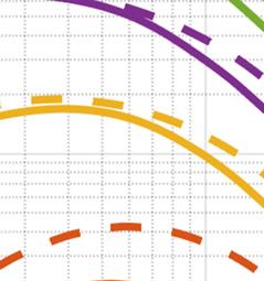
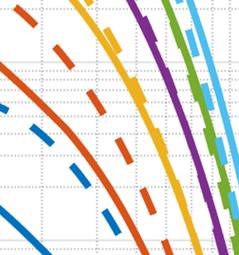
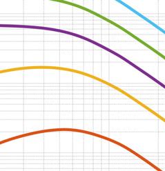
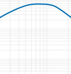
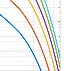
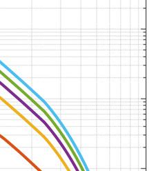
59 6 Model Summary 6.1 MEDIAN MODEL In this section, the median model behavior is summarized. In Figure 6.1, the median EAS spectra from this model (solid lines) are compared with spectra from the additive double-cornerfrequency source spectral model (dashed lines) described in Boore et al. [2014]. The doublecorner-frequency spectra are computed using typical parameters for the WUS given by Boore [2003], including shear-wave velocity 3.5 km/sec, density 2.72 gm/cm 3, stress parameter = 50 bars, and = sec. Also used are the Boore and Thompson [2015] finite-fault distance adjustment, the Boore and Thompson [2014] path duration for western North America, and the Boore [2016] crustal amplification model. The point-source spectral models are calculated using the software package SMSIM [Boore 2005]. The median model spectra are computed for a strike-slip scenario at R RUP = 30 km and Z tor = 0 km, and with the reference Vs 30 and Z 1 conditions. Figure 6.1 shows overall good agreement between the median model and the additive double-corner-frequency source spectral model with typical WUS parameters, including a welldefined decrease in corner frequency with increasing M. At frequencies well below the corner frequency, the spectra should be directly proportional to seismic moment (M 0 ), and since M 0 = M-16.05, the spectra in this range should scale by for one magnitude unit. This approximate scaling is evident in Figure 6.1. At frequencies between Hz, there is a dip in the model spectra compared with the point source spectra. This may be related to the regionspecific attenuation parameters (geometric spreading and Q), where the point source spectra use generalized models for these attenuation parameters. The -based extrapolation in the model spectra begins at 24 Hz. In Figure 6.2, the median EAS spectra from this model are shown for a set of scenarios. Panels (a) and (b) show the spectra for a vertical strike slip scenario at R RUP = 30 km with Vs 30 = 1000 and 500 m/sec, respectively. In (c) and (d) are the spectra for the same Vs 30 but at V but at R RUP = 1 km. In Figure 6.3, the distance scaling of the median model is shown for f = 0.2, 1, 5, and 20 Hz. All spectra in this figure are from a strike slip earthquake rupturing the ground surface with reference Vs 30 and Z 1 conditions. The distance scaling is compared with the Chiou and Youngs [2014] model for PSA (dashed lines) by scaling the PSA values to the R RUP = 0.1 km EAS values. At 0.2 Hz, where the Q term coefficient (c 7 ) is very small, the distance scaling is controlled by the geometric spreading terms, which includes a transition to R -0.5 scaling to model 43

60 surface wave geometric spreading at larger distances. At increasing frequencies, the effect of the Q term becomes more pronounced. In Figure 6.3(d), the distance scaling is shown to deviate significantly from the Chiou and Youngs [2014] model, which has a magnitude dependence on Q. This difference can be explained by the differences between EAS and PSA. At high frequencies, the PSA is strongly influenced by the predominant ground-motion frequency, as discussed above. Because of this, the PSA scaling at 20 Hz and 5 Hz are similar, but since the EAS at 20 Hz is directly representative of the ground motions in that frequency range, the distance scaling is much stronger for 20 Hz than for 5 Hz. The M scaling of the median EAS is shown in Figure 6.4 for a strike slip surface rupturing scenario with reference Vs 30 and Z1 conditions, for f = 0.2, 1, 5, and 20. In Figure 6.5 through Figure 6.7, the median M scaling is compared with that from a set of broadband finitefault simulations. The simulations were performed on the SCEC Broadband Platform, [Maechling et al. 2015] version 17.3, using simulation methods Graves and Pitarka [2015] (also known as GP) and Atkinson and Assatourians [2015] (also known as EXSIM). Both simulation methods were used to develop broadband time histories for vertical strike slip scenarios with a range of M 6.5 to 8 and with stations arranged on constant R RUP bands. In these figures, the M scaling is shown for R RUP = 3, 10, 20, and 30 km for the median EAS model, the GP simulations, the EXSIM simulations, and for the Chiou and Youngs [2014] (CY14 hereafter) model for PSA. For the CY14 PSA, the amplitudes are scaled to the EAS model values at M 6.5 for this comparison. The symbols identified in the legend represent the mean simulated EAS over all stations on a given R RUP band, and the standard error of the mean. The simulations are used to evaluate the near-source saturation of the M scaling and to compare with the scaling implied by the data. Overall, there is less saturation in this GMM than there is in CY14 at all frequencies. At very close distances, there is stronger high-frequency saturation in EXSIM than in GP. Interestingly, this relationship is inverted at low frequencies. Based on these and other comparisons, it is determined the EAS saturation in this model is not inconsistent with the saturation from the simulations. The EAS should have some scaling at zero distance even though the PSA is nearly fully saturated at high frequencies because the PSA procedure involves selecting the peak response of the oscillator over all time, meaning it is not affected by duration. Conversely, the EAS will continue to scale for large magnitudes at short distance due to the longer source durations. The site response scaling of the median model is summarized for a set of example scenarios in Figure 6.8. Panel (a) shows the V s30 scaling of the median model for a M 7 strike slip earthquake rupturing the surface with reference Z 1 conditions at R RUP = 30 km. The solid lines represent the total (linear and nonlinear) V scaling and the dashed lines represent only the linear portion of the V s30 scaling. Panel (b) shows the Z 1 scaling of the median model for the same scenario with V s30 = 300 m/sec. Panel (c) shows the scaling of the modified Hashash et al. [2018] nonlinear site term with M, for a scenario with R RUP = 30 km and V s30 = 300 m/sec. Similarly, panel (d) shows the scaling of the modified Hashash et al. [2018] nonlinear site term with R RUP, for a scenario with M 7 and V s30 = 300 m/sec. 44

61 Figure 6.1 Median model spectra for a strike-slip scenario at R RUP = 30 km, Z tor = 0 km and with reference Vs 30 andd Z 1 conditions (solid lines) compared with the additive double-corner frequency source spectral model with typical WUS parameters (dashed lines). 45

62 Figure 6.2 Median model EAS spectra for a set of scenarios described by the parameters in each title. 46

63 Figure 6.3 Distance scaling of the median EAS (solid lines) for a strike-slip scenario with reference Vs 30 and Z 1 conditions, for four frequencies. For reference, the distance scalingg of the Chiou and Youngs [2014] model for PSA is shown for the same scenarios with the dash- dotted lines, where the PSA valuess have been scaled to the R RUP = 0.1 km EAS values. 47

64 Figure 6.4 M scaling of the median EAS for a strike slip surface rupturing scenario with referencee Vs 30 and Z1 conditions for f = 0.2, 1, 5, and 20 Hz. 48

65 Figure 6.5 M scaling of the median model for four distances, at f = 0.5 Hz for a strike slip earthquake rupturing the surface with referencee Vs 30 and Z 1 conditions, compared with results from finite-fault simulations. 49

66 Figure 6.6 M scaling of the median model for four distances,, at f = 1 Hz for a strikeslip earthquake rupturing the surface with reference Vs 30 and Z 1 conditions compared with results from finite-fault simulations. 50

67 Figure 6.7 M scaling of the median model for four distances, at f = 5 Hz for a strike-slip earthquake rupturing thee surface with reference Vs 30 and Z 1 conditions, compared with results from finite-fault simulations. 51

68 (a) (b) (c) (b) Figure 6.8 (a) V s30 scaling of the median model for a M 7 strike slip earthquake rupturing the surface with reference Z 1 conditions at R RUP = 30 km. The solid lines represent the total (linear and nonlinear) V s30 scaling and the dashed lines represent only the linearr portion of the V s30 scaling; (b) Z 1 scaling of the median model for the same scenario with V s30 = 300 m/sec; (c) scaling of the modifiedd Hashash ett al. [2018] nonlinear site term with M, for R RUP = 30 km and V s30 = 300 m/sec; and (d) scaling of the modified Hashash et al. [2018] nonlinear site term with R RUP P, for M 7 and V s30 = 300 m/sec. 52

69 6.2 STANDARD D DEVIATION MODEL Prediction of the EAS [Equation (3.1)] requires a model for the aleatory variability. The random- (B) site-to-site residuals (S2S) and single-station within-event residuals (WS), which have effects method employed leads to the separation of total residuals into between-event residuals 2 2 variance components, S2S, and SS, respectively. Thee total standard deviation model (natural logarithm units) is given by Equation (6.1) S2S SSc1a (6.1) In Equation (6.1), c 1a is the spectral shape adjustment coefficient (Figure 4.10) which has been added to the total standard deviation, as described previously. Figure 6.9 shows the standard deviations for each component of Equation (6.1), as calculated directly from the regression analysis (all magnitudes). The increase observed in τ at frequencies greater than about 3 Hz is consistent with the behavior of response spectrum models (e.g., Abrahamson et al. [2014] and Chiou and Youngs [2014]). This is believed to be the effect of, which is related to regional crustal damping, being mapped into the between-event terms. For a given earthquake, recordings in close proximity to the source will have similar, andd the high frequencies of these recordings may be systematicall ly above or below average. If there is a regional difference in kappa, then the regression treats this as an event-specific in the variance components off the FAS with increasing frequency and variation, which artificially increases. Stafford [2017] also observed an increase hypothesized that the increase of reflects variations in across different sites. f S2S Figure 6.9 Standard deviation components calculated directly from the regression analysis for all magnitudes. 53

70 The magnitude dependence of each aleatory term is fit as shown in Figure 6.10 and is given by Equation (6.2). At low frequencies, the small-magnitude data have higher betweenevent standard deviation. This is also consistent with the Abrahamson et al. [2014] response spectrum model, and could be related to the steeper magnitude scaling slope at low magnitudes and the uncertainty in small-magnitude source measurements [Abrahamson et al. 2014]. The standard deviations of the two within-event residuals do not have strong magnitude dependence at low frequencies. At higher frequencies, does not show strong magnitude dependence, but S2S and SS are larger for the small-magnitude data, which is again consistent with the Abrahamson et al., [2014] and Chiou and Youngs [2014] models. Higher within-event variability for small magnitudes may be related to the increased effect of the high-frequency radiation pattern, which is reduced for larger magnitude events due to destructive interference [Abrahamson et al. 2014]. s s s3 M M 2 s s 2 for M for for M 6.0 (6.2a) s s S2S s3 M M 4 s s 2 for M for for M 5.5 (6,2b) SS s s s5 M M 6 s s 2 for M for for M 6.0 (6.2c) At frequencies above approximately 20 Hz, the model is constrained to smoothly transition to be flat in frequency space for all components of. The frequency dependence of the standard deviation model is shown in Figure 6.11, and examples of the total standard deviation model for a set of scenarios are shown in Figure Coefficients s 2 through s 2 are given in Appendix B. In Figure 6.13, the components of the standard deviation model are compared with those from Bora et al. [2015] and Stafford [2017]. The Bora et al. [2015] model was developed for smoothed FAS from data in Europe, the Mediterranean, and the Middle-East, and the Stafford [2017] model was developed for unsmoothed FAS from a subset of the NGA-West1 database [Chiou et al. 2008]. The standard deviation model developed here is linear, meaning it does not account for the effects of nonlinear site response. As discussed in Al Atik and Abrahamson [2010] and Abrahamson et al., [2014], the nonlinear effects on the standard deviation are influenced by the variability of the rock motion, leading to a reduction in the soil motion variability at high frequencies. In Abrahamson et al. [2014], the standard deviation of the rock motion is estimated by removing the site amplification variability (determined analytically) from the surface motion, 54

71 and the variability of the soil motion is computed using propagation of errors. In a future update of the model, similar steps will be taken to account for the effects of nonlinear site response on the standard deviation. Figure 6.10 Magnitude scaling of the standard deviation terms for f = 1 and 5 Hz. 55

72 Figure 6.11 Frequency dependence of the standard deviation model. (a) (b) Figure 6.12 (a) Total standard deviation model forr M 3, 5, and 7; and (b) median (solid lines) and median plus and minus onee (dashed lines) EAS spectra for M 3, 5, and 7 scenarios. 56

73 Figure 6.13 Comparison of the standard deviationn components between the Bora et al. [2015], Stafford [2017] models and this model, for a M 5 earthquake. Panels (a) through (d) show the comparison of, S2S, and SS, and, - respectively. 6.3 RANGE OF APPLICABILITY The model is applicable for shallow crustal earthquakess in California and Nevada. The model is developed using a database dominated by California earthquakes, but uses data worldwide to constrainn the magnitude scaling and geometric spreading. The model is applicable for rupture distancess of km, M , and over the frequency range Hz. The V s30 range of applicability is m/sec, although the model is not well constrained for V s30 values greater than 1000 m/sec. Models for the median and the aleatory variability of the EAS are developed. Regional models for Japan and Taiwan will be developed in a future update of the model. A model for the inter-frequency correlation of EAS is presented in Bayless and Abrahamson [2018]. 6.4 LIMITATION NS AND FUTURE CONSIDERATIONS The model presented uses the ergodic assumption, as introduced by Anderson and Brune [1999]. This means that the variability in the data from a broad geographic region (in this case, globally for the magnitude scaling and geometric spreading, andd over the California and Nevada for the 57