Parallel Scalable Iterative Substructuring: Robust Exact and Inexact FETI-DP Methods with Applications to Elasticity

Transcription

1

2

3 Parallel Scalable Iterative Substructuring: Robust Exact and Inexact FETI-DP Methods with Applications to Elasticity Oliver Rheinbach geboren in Hilden Fachbereich Mathematik Universität Duisburg-Essen 29. Mai 2006 Dissertation im Fach Mathematik zum Erwerb des Dr. rer. nat. am Fachbereich Mathematik der Universität Duisburg-Essen

4 Erstgutachter: Prof. Dr. Axel Klawonn, Fachbereich Mathematik, Universität Duisburg-Essen Zweitgutachter: Prof. Dr. Olof B. Widlund, Courant Institute of Mathematical Sciences, New York University Drittgutachter: Prof. Dr. Gerhard Starke, Institut für Angewandte Mathematik, Universität Hannover Tag der mündlichen Prüfung:

5 Contents 1 Introduction Spaces Scalar Partial Differential Equations (PDEs) Weak Formulation and Ellipticity Finite Element Method (FEM) Direct Solvers Krylov Subspace Methods Preconditioned Conjugate Gradient Method (PCG) Generalized Minimal Residual Method (GMRES) Scalability Discrete Harmonic Functions Equivalence of Schur Complement Norm and H 1/2 ( Ω)-Norm Graphs Two Iterative Substructuring Methods A First Model Problem FETI-DP and BDDC with Matrices and Vectors FETI-DP Method BDDC Method Scaling for Heterogeneous Problems Convergence Estimate for FETI-DP and BDDC FETI-DP for Linear Elasticity Equations of Linear Elasticity Need for an Appropriate Coarse Space FETI-DP in 3D Change of Basis Local Lagrange Multipliers Edges Change of Basis for Edge Constraints Choice of Coarse Problem

6 6 CONTENTS Algorithm D E Algorithm D F Optional Lagrange Multipliers Parallel Implementation Distributed Computing and Message Passing Graph Partitioning PETSc Parallel FETI-DP Numerical Results Model Problem Industrial Applications Cancellous Bone Inexact FETI-DP Methods FETI-DP Saddle Point Formulation Exact and Inexact FETI-DP Methods Block Triangular Preconditioners Analysis of the Preconditioners Preconditioning the Original System (ifeti-dp) Preconditioning the Reduced System (irfeti-dp) Performance Considerations Some Technical Remarks Algebraic Multigrid (AMG) Numerical Results Direct Solvers Inexact Coarse Problem Inexact Neumann Problems Inexact Neumann, Dirichlet, and Coarse Problems Parallel Results Conclusions Heterogeneous Elasticity Additional Constraints Necessary and Sufficient Constraints Acceptable Paths Curved Edges Heterogeneities Not Aligned With Interface Conclusions

7 CONTENTS 7 6 Almost Incompressible Elasticity Discretization Coarse Problem Numerical Results Higher Order Methods Spectral Elements Discretization Convergence Estimate Numerical Results for FETI-DP and BDDC hp Finite Elements References 170

8 8 CONTENTS Acknowledgments I would like to thank my advisor Axel Klawonn for the time and work devoted to me and to this thesis as well as for the encouragement he gave me. I am also grateful to Olof Widlund for inspiration and encouragement. I would like to thank both and Gerhard Starke for reviewing this work. Furthermore, I am happy to thank my colleagues at the University of Duisburg-Essen, especially Thomas Schamberg, with whom I have shared an office for many years. I would not have been able to finish this work without the support of my parents and my friends. I am thankful for many fruitful discussions with Barry Smith, Satish Balay, Matthew Knepley, Jason Sarich and the PETSc team, while visiting the Mathematics and Computer Science Division at Argonne National Laboratory, USA. I would also like to thank Panayot Vassilevski, Ulrike Meier Yang, the hypre team and David Keyes at Lawrence Livermore National Laboratory. I am very happy to express my thanks to Barbara Wohlmuth and Luca Pavarino as well as Andrea Toselli and Xavier Vasseur. I enjoyed working with them. I am grateful to Tanja Clees, Klaus Stüben, and the Fraunhofer Institute for Algorithms and Scientific Computing (SCAI), Sankt Augustin, Germany, for providing SAMG and also wish to thank Hans-Jürgen Philipsenburg, Holger Hein and GETRAG FORD Transmissions GmbH, Cologne, Germany. This work gratefully acknowledges the X-ray computer tomography cross sections which were obtained from Matthias Epple, Institute of Inorganic Chemistry, University of Duisburg-Essen, within a common research collaboration. Furthermore, this work gratefully acknowledges the use of Jazz, a 350 node computing cluster operated by the Mathematics and Computer Science Division at Argonne National Laboratory, USA, as part of its Laboratory Computing Resource Center. It also gratefully acknowledges the use of the processor MCR cluster at the Lawrence Livermore National Laboratory, USA. Moreover, for this work computing time was used on the 96 processor Zivcluster of the Universität Münster, Germany, as part of the Rechnerverbund NRW. Additional testing was done, to some extent, on the 256 processor Rubens cluster of the Universität Siegen, the processor ALiCEnext cluster of the Universität Wuppertal, and on our own 16 processor cluster in Essen. Many images in this work were rendered using Medit [48].

9 Chapter 1 Introduction Many complex problems in physics and engineering are described by Partial Differential Equations (PDEs). In general, it is impossible to find exact solutions to these equations, and instead a discrete problem is defined, which represents an approximation of the original problem. Such a discrete problem can be defined, e.g., by using the finite element method (FEM). The discretization then results in large linear equation systems, which today can be of the order of 10 5 to 10 9 unknowns. These linear systems are often too large to be solved exactly. Domain decomposition methods are iterative algorithms to find approximate solutions for the large systems obtained from the discretization of Partial Differential Equations. They make use of underlying properties of the PDEs to achieve fast convergence by applying a hierarchical approach. In domain decomposition methods, the domain associated with the partial differential equation is decomposed into a, possibly large, number of subdomains. In these subdomains, local problems are defined, which are solved in each iteration step in order to define an approximate inverse of the system matrix. In order to obtain a numerical scalable algorithm, also a small coarse problem has to be introduced and solved in each iteration step. The divide-and-conquer approach taken in domain decomposition methods makes them particularly suitable for parallel computing. In this work, we consider nonoverlapping domain decomposition methods belonging to the Dual-Primal Finite Element Tearing and Interconnecting (FETI-DP) methods, originally introduced by Farhat [40]. We will also consider its primal counterpart, the Balancing Domain Decomposition (BDDC) method due to Dohrmann [29], although our presentation will be biased towards the FETI-DP method. We will present FETI-DP algorithms, along with parallel implementations, for compressible homogeneous and heterogeneous 3D linear elasticity, as well as scalar elliptic problems, for almost incompressible elasticity and 9

10 10 CHAPTER 1. INTRODUCTION for higher order methods, i.e. spectral and hp finite elements. Today s distributed memory supercomputers can have up to 10 5 processors. The design of algorithms that can make efficient use of such machines is a challenging task. The standard FETI-DP method is limited in parallel scalability almost exclusively by the exact solution of its coarse problem, see discussion below. We propose a new algorithmic variant, together with a family of inexact FETI-DP methods, which allows for an inexact solution of the FETI-DP coarse problem, and thus remove this limitation of the standard FETI-DP method. The FETI-DP method was originally introduced in Farhat et al. [40] using vertex constraints and extended to 3D in Farhat, Lesoinne, and Pierson [41] using additional, optional average constraints. In Mandel and Tezaur [100], a convergence bound for 2D was provided. Then, in Klawonn and Widlund [84], Klawonn, Widlund, and Dryja [86, 87], and Klawonn and Rheinbach [76] a family of FETI-DP algorithms for 3D together with convergence bounds was introduced. The family of FETI-DP algorithms descended from the earlier one-level and two-level FETI algorithms, see Farhat and Roux [45, 46], Farhat, Mandel, and Roux [43], Farhat and Mandel [42], Farhat, Pierson, and Lesoinne [44]. Already the FETI method has been used in large scale parallel simulations, e.g. [13]. The Dirichlet preconditioner without scaling was first introduced in Farhat, Mandel, and Roux [43]. For early references to the scaled version, see, e.g., Rixen and Farhat [111] and Klawonn and Widlund [83]. Let us note that appropriate scaling is important to obtain convergence results which are independent of jumps in the coefficients of the partial differential equation [83, 86, 84]. But also for homogeneous problems, scaling can be important to improve convergence and also in order to obtain an improved condition number bound, see Mandel and Tezaur [99] and Klawonn and Widlund [83]. FETI methods belong to the larger family domain decomposition methods without overlap, also referred to as iterative substructuring methods; for an introduction, see Smith, Bjørstad, and Gropp [127] and Toselli and Widlund [136]. In FETI-DP methods the continuity of the solution across the subdomain boundaries is enforced by Lagrange multipliers. This results in a mixed linear system with primal variables and Lagrange multipliers as unknowns. The basic idea of FETI-DP domain decomposition methods is to form a Schur complement by eliminating the primal variables and then iterate on the Lagrange multiplier variables, usually in combination with a preconditioner. Special attention has to be given to the elimination process of the primal variables since the associated local matrices are usually only semidefinite even though the overall mixed linear system is uniquely solvable. This is

11 due to local stiffness matrices belonging to subdomains lacking sufficient essential boundary conditions. In FETI-DP methods, a sufficient number of constraints, e.g. continuity constraints across the interface at selected nodes on the subdomain boundaries, is chosen such that the local stiffness matrices become invertible. We note that nodal constraints work well only in two dimensions, more elaborate choices, e.g. averages over edges or faces, are used in three dimensions in order to obtain a good convergence estimate, see Chapters 2 and 3. These additional primal constraints introduce a certain coupling between the otherwise completely decoupled local subdomain problems. This coupling also builds the coarse problem needed for scalability of the algorithm. FETI-DP methods obtain their numerical and parallel scalability from the fact that the coarse problem is very small compared to the overall problem. This coarse problem is traditionally solved exactly by the use of a direct solver. Nevertheless, if a very large number of subdomains is used or if the problem requires the use of a larger coarse space, the cost of solving the coarse problem directly may become high. In standard FETI-DP methods, an inexact solution of the coarse problem is not straightforward since the coarse problem is, by means of the elimination process, built into the FETI- DP system matrix. Thus, an inexact solution in the elimination process of the primal variables would lead to a different linear system to be solved and thus to a perturbed solution, different to that of the original problem. Another class of nonoverlapping domain decomposition methods, which is closely related to the FETI-DP algorithms, are the Balancing Domain Decomposition methods by Constraints (BDDC); see Cros [26], Dohrmann [29], Mandel and Dohrmann [97], Mandel, Dohrmann, and Tezaur [98], or Li and Widlund [92]. We note that there are also FETI methods using two sets Lagrange multipliers; see, e.g., Magoulès, Roux, and Salmon [95], Magoulès, Roux, and Series [96], or Series, Feyel, and Roux [121]; there are also other domain decomposition methods using Robin boundary conditions at the interface; see, e.g., Flauraud and Nataf [47] and the references given therein. In Chapter 1 we have collected background material that may be helpful for the reader. In Chapter 2 we introduce the FETI-DP and BDDC method and also sketch the theory for the 2D scalar case to motivate our work on 3D linear elasticity in Chapter 3. There, we describe a FETI-DP algorithm for 3D linear elasticity along with an efficient parallel implementation, for which the theory was provided in Klawonn and Widlund [84]. We show the numerical and parallel scalability of the algorithm for academic benchmark problems as well as for more general situations with unstructured meshes from engineering problems where the theory does not apply. In Chapter 4 11

12 12 CHAPTER 1. INTRODUCTION we introduce new, inexact FETI-DP algorithms. Here, different subproblems within the FETI-DP method can be solved approximately. Of particular interest is a version denoted irfeti-dp which allows for an inexact solution of the FETI-DP coarse problem. Using this approach the parallel scalability of FETI-DP algorithms can be extended further. We provide sequential and parallel experiments to demonstrate the high potential of the method and its applicability to problems with more than 10 4 subdomains. In Chapter 5 we describe a FETI-DP algorithm for elasticity with jumps in the material coefficient, also motivated by the theory in [84]. We investigate the effect of different material distributions guided by the theory and try to develop rules for more general cases than covered by the theory. In Chapter 6 we treat the case of two dimensional almost incompressible elasticity, and in Chapter 7 we apply our FETI-DP methods to spectral and hp finite element discretizations. We also show numerical and parallel scalability for the FETI- DP and irfeti-dp methods applied to spectral element discretizations. The present chapter contains background material which is frequently needed in the presentation and analysis of the FETI method in subsequent chapters. 1.1 Spaces Let Ω R d, d = 2, 3 be a bounded Lipschitz domain. We will be particularly interested in polygonal and polyhedral domains. Throughout this work we will refer to the diameter of a subdomain by H. Define L 2 (Ω) as the usual space of square integrable functions with the norm u 2 L 2 (Ω) = u 2 dx. We have the standard Sobolev space H 1 (Ω) as the space of functions which are square integrable as well as their first derivatives in the sense of distributions. Furthermore, we have the H 1 (Ω)-seminorm as u 2 H 1 (Ω) = u, u dx. We obtain a weighted norm suitable for our purposes by Ω u 2 H 1 (Ω) = u 2 H 1 (Ω) + H 2 u 2 L 2 (Ω), where we introduce the weight factor to avoid undesirable scaling effects. We mention only briefly that the norms come from the corresponding inner Ω

13 1.1. SPACES 13 products. We want to set essential boundary conditions on elements of H 1 (Ω). We denote C0 (Ω) the infinitely differentiable functions with support in Ω. As the closure of C0 (Ω) in H 1 (Ω) we obtain the space H0(Ω). 1 We recall that Sobolev spaces on manifolds can be introduced using sufficiently smooth maps and a partition of unity. Most notably, we will need the trace of H 1 (Ω) on the domain boundary. The intrinsic H 1/2 (Γ)-seminorm for Γ Ω is given by u 2 H 1/2 (Γ) = u(x) u(y) 2 dγ(x)dγ(y) x y d and the properly weighted norm on Γ by Γ Γ u 2 H 1/2 (Γ) = H 1 u 2 L 2 (Γ) + u 2 H 1/2 (Γ). Then, H 1/2 ( Ω) is the trace space of H 1 (Ω) on the domain boundary. Note that an equivalent seminorm is given by as a result of the following theorems. u 2 H 1/2 (Γ) = min v Γ =u v 2 H 1 (Ω) (1.1) Theorem (Trace Theorem) If Ω is a bounded Lipschitz domain, then the trace operator γ : u γu, which represents the restriction of u to the boundary of Ω, is a continuous mapping from H 1 (Ω) onto H 1/2 ( Ω). This implies γu 2 H 1/2 ( Ω) C(Ω) u 2 H 1 (Ω). For a reference, see, e.g., [58, Theorem , p. 38]. This inequality remains valid if we substitute the norm by the seminorm. Note that, due to the chosen scaling, we obtain γu 2 L 2 ( Ω) C(Ω) ( H 1 u 2 L 2 (Ω) + H u 2 H 1 (Ω) ). We also have a family of extension theorems. Theorem (Extension Theorem) There is a continuous extension operator from H 1/2 ( Ω) to H 1 (Ω), u û, therefore û H 1 (Ω) C(Ω) u H 1/2 ( Ω).

14 14 CHAPTER 1. INTRODUCTION The harmonic extension, see Section 1.6, defines a continuous mapping in this sense. Sometimes we will identify functions from H 1/2 ( Ω) with their harmonic extension to the interior. The following well known inequalities, which establish the equivalence of norms in subspaces of H 1 (Ω), are essential to us, see [102]. Theorem (Friedrichs Inequality) There exists a constant C(Ω) > 0 such that u 2 H 1 (Ω) C(Ω) u 2 H 1 (Ω) for all u H 1 (Ω, Γ) = {u H 1 (Ω) : u = 0 on Γ}, where Γ Ω is a surface with positive measure. Theorem (Poincaré Inequality) There exists a constant C(Ω) > 0 such that ( u 2 H 1 (Ω) C(Ω) u 2 H 1 (Ω) + 1 ( ) ) 2 u dx H 2+d Ω for all u H 1 (Ω). There are also Poincaré inequalities in H 1/2 (Ω). An additional space is relevant to this work since we want to consider isolated faces or edges of polyhedral domains. Let Γ be an open subset of Ω and u H 1/2 (Γ). Then the extension of u by zero from Γ to Ω does not define a continuous operator from H 1/2 (Γ) to H 1/2 ( Ω), see [58, pp. 18f, Lemma ]. Therefore, we consider the space H 1/2 00 (Γ), defined as the set of all functions u H 1/2 (Γ) for which the continuation of u from Γ to Ω with zero, denoted by ũ, remains bounded in H ( Ω). Thus, we have 1/2 H 1/2 00 (Γ) = {u L 2 (Γ) ũ H 1/2 ( Ω)}. The space H 1/2 00 (Γ) is a subspace of H 1/2 0 (Γ) and complete with the norm inherited from H 1/2 ( Ω) [58, pp. 18f, Lemma ]. For our finite element functions, which are continuous by construction, this subtle difference disappears and we can either write u 2 or H 1/2 00 (Γ) u 2. H 1/2 ( Ω) Another equivalent norm for H 1/2 00 (Γ) is given by u 2 = H 1/2 00 (Γ) u 2 H 1/2 (Γ) + u 2 d(x; Γ) 1 dx, where d(x; Γ) denotes the distance from x to the boundary of Γ, see [58, pp. 18f]. Γ

15 1.2. SCALAR PARTIAL DIFFERENTIAL EQUATIONS (PDES) Scalar Partial Differential Equations (PDEs) Weak Formulation and Ellipticity We obtain the weak formulation of a scalar partial differential equation of the type i (a ij (x) j u) = f in Ω, (1.2) i,j u = 0 on Ω D Ω, (1.3) and a ij (x) j uν i = g on Γ N = Ω \ Ω D, (1.4) i,j where ν is the outward normal to Ω, by means of a Green s formula. We get a ij (x) i v j u dx = fv dx + gv ds, (1.5) Ω Ω Ω N i,j for all v H 1 0(Ω, Ω D ) := {v H 1 (Ω) : v = 0 on Ω D }. The differentiation is to be understood in the variational sense. We introduce the symmetric bilinear form a(u, v), the linear form f(v), and the Hilbert space to write (1.5) in the compact form V := H 1 0(Ω, Ω D ) a(u, v) = f(v) v V. (1.6) The Lemma of Lax-Milgram guarantees that the problem (1.6) has a unique solution if a(, ) is continuous, a(u, v) C u v u, v V, elliptic α > 0 : a(u, u) α u 2 u V, and f( ) is continuous, f(v) C v v V.

16 16 CHAPTER 1. INTRODUCTION nz = Figure 1.1 Linear basis functions and a linear combination in one dimension (left). Sparsity pattern of a stiffness matrix for a 3D problem (right) Finite Element Method (FEM) Consider the weak formulation of a homogeneous second order elliptic problem, e.g. the scalar equation Z X Z aij (x) i u j v dx = f v dx v V, (1.7) Ω i,j Ω or in compact notation a(u, v) = (f, v) v V. (1.8) In the finite element method we replace the infinite dimensional function space V by a finite dimensional subspace V h, e.g. the space of piecewise linear continuous functions. This yields a(uh, vh ) = (f, vh ) vh V h. (1.9) P The basis representation uh = i ui φi leads to the linear equation system Ku = b, ³ ³ where K = a(φi, φj ) and bi = (f, φi ). The matrix is symmetric positive definite if the bilinear form a(, ) is symmetric and V -elliptic, and it is sparse since the basis functions only have a local support. The number of nonzero entries is generally O(n) if the size of K is n n.

17 1.3. DIRECT SOLVERS Direct Solvers The simplest algorithm to solve a system of linear equations Ax = b, where A R m m, is the well known Gaussian elimination, for i=1..m for j=i+1..m for k=i+1..m a(j,k)=a(j,k)-a(i,k)*a(j,i)/a(i,i) end end end, which requires O(m 3 ) operations. Here, we have given the Gaussian elimination in its simplest, so called right-looking, form. Finite element stiffness matrices are typically sparse since the basis functions of the finite element space are local. Hence, it is more efficient to store only nonzeros entries in the matrix. The Gaussian elimination then takes the form for i=1=1..n for j=nextnonzeroindex(j) for k=nextnonzeroindex(k) a(j,k)=a(j,k)-a(i,k)*a(j,i)/a(i,i) end end end. Here, the computational cost has been significantly reduced but during the elimination process some entries in A which were previously zero become nonzero. These new entries are referred to as fill-in. The amount of fill-in in the elimination process depends on the ordering of the matrix and increases the computational cost. Let us assume that we can order our matrix in a way that it has the following block structure K (1) II K (1) IΓ.... K (N) II K (1) ΓI K(N) ΓI K (N) IΓ K ΓΓ [ = K II K ΓI We have chosen this notation because we can think of the matrices K (i) II as subdomain interior matrices and of K ΓΓ as the global interface matrix. All KIΓ KΓΓ ].

18 18 CHAPTER 1. INTRODUCTION the matrices K (i) II can be factored independently (possibly also in parallel), and no fill-in will appear in the off-diagonal blocks of K (1) II... K (N) II Then, finally, the Schur complement S = K ΓΓ K ΓI K 1 K II IΓ has to be formed and the Schur complement system has to be solved. The matrix S contains many dense blocks and we could perform this last step even by using dense Gaussian elimination, see above. Moreover, we can apply this approach recursively to K (i) II until our subdomains become single matrix entries. For this approach to be efficient, the matrix K ΓΓ should be small. Unfortunately, the problem to find the optimal interface, also called separator, is NP complete. Therefore, different strategies have been developed to find good orderings of K, e.g. nested dissection (ND) [50] and minimum degree (MD/AMD) [51, 27] orderings and many variants thereof. In finding good separators, direct solvers have also benefitted, as have iterative substructuring methods, from advances in graph partitioning software. Applying optimal orderings, the complexity of directly solving linear systems resulting from finite element discretizations can be reduced to O(m 3/2 ) in 2D and O(m 2 ) in 3D. The design and the implementation of efficient direct solvers is a challenging task, and significant progress has been made in recent years. Today several efficient direct solver packages are available. Among them are MUMPS [5] and UMFPACK [27], which both use the multifrontal approach [33]. The package UMFPACK is a sequential code whereas MUMPS is also targeted at distributed memory parallel computers. We have also used Spooles [7] and SuperLU Dist [93]. The latter is the distributed memory version of the supernodal direct solver package SuperLU. Other (sequential and parallel) direct solvers, not available in source code, are WSMP [64] and PARDISO [115] Krylov Subspace Methods Domain decomposition methods are commonly used as preconditioners for the use with Krylov subspace methods. We will briefly describe the two methods which are of most relevance to this work. For further details, refer to Saad [113], Greenbaum [57], and many others. It is well known that

19 1.4. KRYLOV SUBSPACE METHODS 19 for well conditioned problems the performance of different Krylov subspace methods is very similar Preconditioned Conjugate Gradient Method (PCG) Let us consider a symmetric positive definite linear system Ax = b. (1.10) The Preconditioned Conjugate Gradient (PCG) method is an iterative method to solve (1.10) by minimizing 1 2 xt M 1/2 AM 1/2 x x T M 1/2 b, over a certain Krylov subspace; see, e.g. [113, 57, 123]. Here, the symmetric operator M 1 is the preconditioner for A. The convergence of the PCG method is governed by the eigenvalues of M 1 A, i.e. x (k) x A x (0) x A 2 ( κ(m 1 A) 1 κ(m 1 A) + 1) k, where κ(m 1 A) = λmax(m 1 A) λ min (M 1 A) is the condition number of M 1 A. Both, the system matrix A as well as the preconditioning matrix M 1, are only needed in matrix vector multiplications. Therefore, M 1 x as well as Ax must be easy to compute, and the condition number κ(m 1 A) should be small. If elliptic partial differential equations of second order are discretized with the finite element method, the system matrix is generally not well conditioned, i.e. the condition number of A is proportional to 1/h 2, where h is a measure of the element diameter. In higher order methods the system matrices can be even more ill conditioned, and the condition number depends on the polynomial degree. However, for an efficient algorithm the condition number of M 1 A should be scalable with respect to the mesh size and, possibly, also with respect to the spectral degree of the discretization. This is the case for the iterative substructuring methods discussed in this work and also for other domain decomposition methods and subspace correction schemes. In this work, whenever conjugate gradients are mentioned, we actually refer to the Preconditioned Conjugate Gradient method.

20 20 CHAPTER 1. INTRODUCTION Generalized Minimal Residual Method (GMRES) The Generalized Minimal Residual (GMRES) method [114] is an iterative method to solve an unsymmetric linear system Ax = b by minimizing the residual over a certain Krylov subspace. If a preconditioner M 1 is available, either left of right preconditioning can be used with GMRES. As opposed to conjugate gradients, where a three term recurrence is used, the work and storage grows linearly with the number of iterations. A full basis for the Krylov subspace has to be computed and stored. Therefore, often a truncated version (restarted GMRES) is applied. Unlike in CG, the convergence behavior of GMRES cannot be described by the eigenvalues alone. If the field of values { } y T M 1 Ay F (A) := : y R n y T y is contained in a disk in the complex plane of diameter s which is centered at c then, see [57], ( ) k r k s r 0 2. c For symmetric preconditioners M 1 in [128] an estimate similar to a classical bound by Elman [34] has been given, r k ( r 0 1 F ( M 1 A ) F ( (M 1 A) 1)) k/2. For block triangular preconditioners in [80] a field of value analysis has been given, using equivalent norms. 1.5 Scalability We are interested in solving linear equation systems obtained from the discretization of partial differential equations. We consider an algorithm scalable if the computational work to find a solution of a prescribed accuracy, e.g. an accuracy of 10 7, grows linearly with the size of the linear system, i.e. the number of degrees of freedom (d.o.f.). In domain decomposition methods accelerated by a Krylov subspace methods like CG or GMRES, if we neglect the computational work for the small coarse problem, we have scalability in this sense if the number of iterations

21 1.6. DISCRETE HARMONIC FUNCTIONS 21 is independent of the problem size. For CG this is the case if the condition number is bounded independently of the number of subdomains. Additionally, we require for our domain decomposition methods that the number of iterations only depends weakly, i.e. polylogarithmically, on the diameter of the subdomains. This gives us some freedom to choose the subdomain sizes. If a domain decomposition method fulfills these two conditions, we call it numerically scalable. We also consider two types of parallel scalability. In the first, we consider a problem of fixed size and increase the number of processors used to solve the problem. An algorithm is parallel scalable if, ideally, twice as many processors will solve the problem in half the time. In the second type of scalability, which is sometimes called weak scalability, we double the problem size and the number of processors at the same time. We then require that, in a parallel scalable algorithm, the solution time is independent of the problem size. The first type of scalability is generally more difficult to achieve in real world applications. The second type of scalability has become important with the advent of massively parallel computers. It explains why supercomputers with thousands of processors can still be used efficiently. 1.6 Discrete Harmonic Functions Let us recall that in the same way as the harmonic functions in H 1 (Ω) are identified through the orthogonality to H 1 0(Ω), ( u, v) = 0 v H 1 0(Ω), (1.11) the discrete harmonic functions are identified through ( u h, v h ) = 0 v h V h 0 (Ω), (1.12) or explicitly K II u I + K IΓ u Γ = 0. This expresses the orthogonality of the functions associated with the the boundary values and the interior functions in the norm defined by the symmetric positive definite stiffness matrix ( ) KII K K = IΓ. K ΓI K ΓΓ The subscript Γ refers to boundary variables and the subscript I to interior variables. It follows from the orthogonality that harmonic and discrete harmonic functions are the extensions of their boundary values with minimal energy in

22 22 CHAPTER 1. INTRODUCTION their respective spaces. For the harmonic function u and discrete harmonic function u h, we have and since for u v H 1 0(Ω) u H 1 (Ω) = inf v H 1 v u H0 1(Ω) (Ω) (1.13) u h H 1 (Ω) = inf v h u h V h 0 (Ω) v h H 1 (Ω), (1.14) ( v, v) = ( (v u + u), (v u + u)) ( u, u) (1.15) is true as well as the analogous result for u h. We denote the discrete harmonic extension of a function u H 1/2 ( Ω) to the interior by Hu H 1 (Ω). 1.7 Equivalence of Schur Complement Norm and H 1/2 ( Ω)-Norm Assuming that Ω is a Lipschitz domain, the seminorm defined by the Schur complement is equivalent to the properly scaled H 1/2 ( Ω)-seminorm. See [16], the extension in [143], and see also [136]. Considering the bilinear form ρ u, v dx, Ω related to the Poisson equation with a constant coefficient ρ, we obtain 1.8 Graphs 1 C ρ u h 2 H 1/2 ( Ω) u h 2 S Cρ u h 2 H 1/2 ( Ω). (1.16) A graph or undirected graph G is an ordered pair G = (V, E), where V N is the set of nodes, and E is a set of unordered pairs {v 1, v 2 }, where v 1, v 2 V are nodes. The elements of e = {v 1, v 2 } of E are called edges. We say that nodes v 1 V and v 2 V are connected through the edge e if e = {v 1, v 2 } E. A path from v 1 V to v 2 V is a list of nodes, starting with v 1 and ending with v 2, where all pairs of consecutive nodes are connected through

23 1.8. GRAPHS 23 edges. If a path from v 1 V to v 2 V exists, we say that v 1 and v 2 are connected in G. Connectivity is an equivalence relation over V and the equivalence classes are called connectivity components of G. Efficient (sequential) algorithms exist to compute connectivity components of graphs, i.e. depth first search or breadth first search, see any introduction into efficient algorithms, e.g., [120], and also [2]. A simple path in G is a path in G, where no node v V is repeated. A cycle in G is a simple path, where start and end node coincide. We call a graph without cycles a forest and a connected forest a tree. A subgraph G = (Ṽ, Ẽ) of G = (V, E) is a graph where Ṽ V and Ẽ E. We say the subgraph G spans G if Ṽ = V. A spanning tree of G = (V, E) is a subgraph of G = (V, E) which spans G and is a tree. A minimal spanning tree is a spanning tree with the smallest possible number of edges. Sometimes a cost function can be associated with edges, in this case the spanning tree minimizes the sum of the edge costs. Efficient algorithms are known to calculate minimal spanning trees. A graph is planar if it can be drawn in a plane with no crossing edges.

24 24 CHAPTER 1. INTRODUCTION

25 Chapter 2 Two Iterative Substructuring Methods In this chapter, we describe the two well known iterative substructuring methods relevant for this work. For simplicity, we will introduce the algorithms in the context of 2D scalar elliptic problems, and we will also sketch the convergence theory in this context based on publications of several other authors [100, 84]. This will serve as motivation for our main work on 3D elasticity problems in Chapter 3 and 5. Dual-primal FETI (FETI-DP) methods are the most recent members of the family of Finite Element Tearing and Interconnecting (FETI) domain decomposition methods. The FETI methods, introduced by Farhat and Roux [45], are dual iterative substructuring methods for partial differential equations. In these methods the original domain, on which the given partial differential equation has to be solved, is decomposed into nonoverlapping subdomains. The intersubdomain continuity is then enforced by Lagrange multipliers across the interface defined by the subdomain boundaries. For further results and references, see, e.g., [46, 38, 13, 99, 83, 136]. In dual-primal FETI methods, some continuity constraints on the primal displacement variables are forced to hold throughout iterations, as in primal substructuring algorithms, while the other constraints are enforced by the use of Lagrange multipliers, as in FETI. The primal constraints have to be chosen such that the local subproblems become invertible and such that a parallel scalable method is obtained. The primal constraints provide a coarse problem for these domain decomposition methods. Dual-primal FETI (FETI-DP) algorithms were introduced by Farhat et al. in [40] for linear elasticity problems in the plane and then extended by Farhat, Lesoinne, and Pierson [41] to three dimensional elasticity problems; see also Pierson [107]. The first theoretical analysis for two dimensional, 25

26 26 CHAPTER 2. TWO ITERATIVE SUBSTRUCTURING METHODS scalar elliptic partial differential equations of second and fourth order with only small coefficient jumps across the subdomain boundaries was given by Mandel and Tezaur [100]. It was shown that the condition number is bounded polylogarithmically as a function of the dimension of the individual subregion problems. The family of algorithms for scalar, second order elliptic problems in three dimensions was extended by Klawonn, Widlund, and Dryja [82, 86, 87]; see also [136]. There, constraints on averages over subdomain edges and faces are used to obtain algorithms with an improved scalability for three dimensional problems. In [41, 107] similar constraints on averages are used for linear elasticity problems, although the definition of subdomain edges is different from the one used in [82, 86, 87], see also the discussion in Section We also note that an important feature of the algorithms presented in [82, 86, 87] was to develop variants of FETI-DP with smaller coarse problems while still maintaining scalability and a good convergence bound. In fact, in [86, 87] a theory was provided which shows that the condition number in three dimensions can again be bounded polylogarithmically as a function of the dimension of the individual subdomain problems and that the bounds can otherwise be made independent of the number of subdomains, the mesh size, and the jumps in the coefficients. More recently, new variants of FETI-DP for three dimensional, linear elasticity problems were provided by Klawonn and Widlund [84, 85] together with a theoretical analysis proving a polylogarithmic condition number estimate as in the scalar case which is also robust with respect to discontinuities in the material coefficients. For benign elasticity problems, it is shown that selecting an appropriate set of edge averages as primal constraints is sufficient to obtain good polylogarithmic bounds. For arbitrary coefficient distributions, certain first order moments on selected edges have to be added as primal constraints as well as constraints at some of the vertices in order to obtain robust, polylogarithmic bounds. Strongly related to FETI-DP methods are the more recently developed Neumann-Neumann methods with constraints, also known as the Balancing Domain Decomposition methods by Constraints (BDDC); cf. [29, 97, 98]. Neumann-Neumann methods with primal vertex constraints were also developed independently by Cros [26]. It was first proved in Mandel, Dohrmann, and Tezaur [98] that the eigenvalues of BDDC and FETI-DP, which are not one or zero, are the same; see also Li and Widlund [92] and Brenner and Sung [20] for other approaches. Recently, new results for inexact FETI-DP and BDDC algorithm have been obtained for the inexact solution of the subdomain or coarse problems. For inexact BDDC methods, see Tu [138, 139, 140], Dohrmann [31], and Li and Widlund [91], and for inexact FETI-DP algorithms, see Chapter 4.

27 Figure 2.1 MCR supercomputer at Lawrence Livermore National Laboratory (Image: Lawrence Livermore National Laboratory, California, USA). 27

28 28 CHAPTER 2. TWO ITERATIVE SUBSTRUCTURING METHODS 2.1 A First Model Problem We will first use a simple model problem in order to define the setting for our presentation of the FETI-DP method and the Neumann-Neumann method with constraints, also known as the BDDC method. Later we will consider the equations of linear elasticity. By using a change of basis, if necessary, the presentation of the algorithms at the level of linear algebra can be the same for all second order elliptic PDEs, but the theory is significantly easier to present for scalar equations. Note that the choice of the primal constraints depends in the spatial dimension and the problem type. Our presentation will be biased towards the FETI-DP method. Since Mandel and Dohrmann [98] have shown that FETI-DP and BDDC share all but possibly two of their eigenvalues, this is not a limitation. See also Li and Widlund for a proof which is closer to our notation. Already in Klawonn and Widlund [83] a common theory for methods of the older FETI and Neumann-Neumann type has been given. We consider the following second order scalar elliptic problem in a two dimensional region Ω R 2 : Find u H0(Ω, 1 Ω D ) such that ρ(x) u v dx = fv v H0(Ω, 1 Ω D ). Ω We decompose Ω into N nonoverlapping subdomains Ω i, i = 1,..., N, i.e. Ω = Ω N Ω i, Ω i Ω j = if i j. i=1 Each subdomain is the union of shape-regular finite elements with matching finite element nodes across the interface, Γ := i j Ω i Ω j, where Ω i, Ω j are the boundaries of Ω i, Ω j, respectively. These subdomains are also often referred to as substructures. The coefficient ρ(x) > 0 can be discontinuous but should have large coefficient jumps only across the interface. In the standard theory it is assumed that ρ(x) is constant on each subdomain. Later, we will see in our numerical simulations that this assumption is in fact too strong, and in many cases large coefficient jumps within subdomains can be allowed without affecting the convergence of the method at all. We assume that subdomains are shape regular and have a typical diameter of H whereas the finite elements are of typical diameter h. We will use low

29 2.1. A FIRST MODEL PROBLEM 29 order conforming finite elements, i.e. linear or bilinear finite elements. In Chapter 7 we will also consider higher order, hp or spectral, elements. We define the bilinear form a(u, v) := ρ(x) u v dx and the functional Ω f(v) := Ω fv dx. We denote by Wg h := Wg h (Ω) the conforming finite element space of finite element functions. The associated discrete problem is then a(u h, v h ) = f(v) v h W h g. (2.1) When there is no risk of confusion, we will drop the subscript h. Moreover, we will often identify the finite element function u h and the corresponding vector u = (u 1,..., u n ) T R n, where u h = N i=1 u iφ i, and where φ 1,..., φ N is the finite element basis we choose to work in. For each subdomain Ω i we will denote the finite element space by W i. In iterative substructuring algorithms the interior variables in each subdomain are eliminated using a direct solver. It is therefore helpful to partition W i into the interior part W (i) I and the finite element trace space W (i) Γ, i.e. we have W i = W (i) I W (i) Γ. Note that we consider variables on the Neumann boundary Ω N as interior to a subdomain. Also, subdomains not intersecting Ω D lack essential boundary conditions and will have singular stiffness matrices. We introduce the product spaces N W := and W Γ := i=1 N i=1 W i W (i) Γ. The members of W and W Γ are in general not continuous across the interface. However, we expect our global solution to be continuous. We therefore consider the subspace formed by the continuous functions in W, which we denote by Ŵ, i.e. we have Ŵ := {w W : w is continuous across Γ}.

30 30 CHAPTER 2. TWO ITERATIVE SUBSTRUCTURING METHODS We also define ŴΓ as the subspace formed by the continuous members of W Γ, i.e. Ŵ Γ := {w Γ W Γ : w Γ is continuous across Γ}. In our iterative substructuring methods, we will iterate in the space W while requiring certain constraints to hold throughout the iteration. In FETI-DP methods these constraints are continuity constraints, also called primal constraints, that have to be chosen such that each subdomain problem becomes invertible and that also a good convergence bound can be obtained. We denote the space of finite element functions which fulfill these constraints by W. We have Ŵ W W, and likewise Ŵ Γ W Γ W Γ. The continuity constraints posed on W only affect a subset of the variables, these variables are denoted as primal. We can decompose W Γ into the primal space W Π = N i=1 W (i) Π and the dual space W = N i=1 W (i), i.e. W Γ = W Π W. Using this notation, we can now decompose W Γ into the subspace ŴΠ which has continuous members only and the subspace W which also contains finite element functions which are not continuous, i.e. we have Likewise, we can now write W Γ = ŴΠ W. Ŵ = ŴΠ Ŵ W I. Here, Ŵ is the subspace formed by the continuous finite element functions in W. For convenience, we also introduce the nonprimal space W B = W W I and Ŵ B = Ŵ W I. 2.2 FETI-DP and BDDC with Matrices and Vectors We will now introduce a matrix formulation of the FETI-DP and the BDDC method.

31 2.2. FETI-DP AND BDDC WITH MATRICES AND VECTORS 31 As we consider a domain Ω R 2, the interface Γ is the union of edges and vertices. In the continuous setting, we regard edges in 2D as open sets that are shared by two subdomains, and vertices as endpoints of edges, see, e.g. Toselli and Widlund [136, Chapter 4.2]. In Chapter 3 we give a detailed definition of vertices, edges, and faces in 3D which is also suitable for irregular domain decompositions. For each subdomain Ω i, i = 1,..., N, we assemble the local stiffness matrices K (i) and load vectors f (i). We denote the unknowns on each subdomain by u (i). We then partition the unknowns u (i) into interface variables u (i) Γ, i.e. unknowns which are associated with the interface Γ, and interior unknowns u (i) I, which are interior to the subdomain Ω i. Note that any variable on Ω N \ Γ is considered to be interior to a subdomain. Unknowns on Ω D are usually eliminated upfront and do not need to be considered. We then partition the interface variables into primal variables u (i) Π and dual variables u (i). In two dimensional problems the primal variables u(i) Π will be associated with vertex unknowns. Vertex unknowns are also often referred to as corner variables. In a structured decomposition of a unit square into smaller squares, the vertex unknowns are all degrees of freedom (d.o.f.) which are associated with nodes shared by four subdomains. Together, interior and dual unknowns form the nonprimal variables u (i) B. In the FETI-DP algorithms we will enforce the continuity of the solution by global subassembly of the subdomain stiffness matrices K (i). For all other interface variables u (i) we will introduce Lagrange multipliers to enforce continuity. We also partition the stiffness matrices according to the different sets of unknowns, in the primal unknowns u (i) Π and K (i) = [ K (i) BB = [ K (i) BB K (i) ΠB K (i) II K (i) I K(i)T ΠB K (i) ΠΠ K (i)t I K (i) ] ], f (i) = [, f (i) B = [ f (i) B f (i) Π f (i) I f (i) We will refer to the completely assembled global stiffness matrix as K g FETI-DP Method We define the block matrices K BB := diag N i=1(k (i) BB ), ] ],.

32 32 CHAPTER 2. TWO ITERATIVE SUBSTRUCTURING METHODS and the right hand sides K ΠB := diag N i=1(k (i) ΠB ), K ΠΠ := diag N i=1(k (i) ΠΠ ), fb T := [f (1)T B,..., f (N)T B ], fπ T := [f (1)T Π,..., f (N)T Π ]. By assembly of the local subdomain matrices in the primal variables using the operator RΠ T = [R(1)T Π,..., R(N)T Π ] with entries 0 or 1, we have the partially assembled global stiffness matrix [ ] [ ] [ ] [ ] K K = BB KT ΠB IB 0 KBB K = T KΠΠ 0 RΠ T ΠB IB 0 K ΠB K ΠΠ 0 R Π K ΠB and right hand side f = [ ] [ fb IB 0 = f Π 0 RΠ T ] [ fb f Π ]. Choosing a sufficient number of primal variables u (i) Π to constrain our solution, for example all vertex unknowns, results in a symmetric positive definite matrix K. We note that the upper left block of K = [ K BB K ΠB KT ΠB KΠΠ is block diagonal and coupling is introduced only through the primal variables. To enforce continuity on the remaining interface variables u (i) we introduce a jump operator B B with entries 0, 1 or 1 and Lagrange multipliers λ. We can now formulate the FETI-DP saddle-point problem K BB KT ΠB B T B K ΠB KΠΠ 0 B B 0 0 u B ũ Π λ ] = f B f Π 0. (2.2) By eliminating u B and u Π from the system (2.2) we obtain the linear system F λ = d,

33 2.2. FETI-DP AND BDDC WITH MATRICES AND VECTORS 33 where F := [ B B 0 ] [ K BB KT ΠB K ΠB KΠΠ d := [ B B 0 ] [ K BB KT ΠB K ΠB KΠΠ ] 1 [ B T B 0 ], ] 1 [ fb f Π ]. From [ K BB K ΠB KT ΠB KΠΠ ] 1 = [ IB K 1 BB K T ΠB 0 I Π ] [ K 1 BB 0 0 S 1 ΠΠ ] [ I B 0 K ΠB K 1 BB I Π ] we conclude that F = B B K 1 BB BT B + B B K 1 BB K BΠ S 1 ΠΠ K ΠB K 1 d = B B K 1 BB f B + B B K 1 BB K T ΠB BB BT B, S 1 ΠΠ ( f Π K ΠB K 1 BB f B). In the standard, exact FETI-DP methods two different preconditioners for F are commonly used, the theoretically almost optimal Dirichlet preconditioner M FETID and the lumped preconditioner M FETIL. We define additional block matrices The Dirichlet preconditioner M FETID K II := diag N i=1(k (i) II ), K I := diag N i=1(k (i) I ), K := diag N i=1(k (i) ). is then defined by (2.3) M 1 FETI D := B B,D (R B ) T (K K I K 1 II KT I)R B B T B,D (2.4) and the lumped preconditioner M FETIL by where M 1 FETI L = B B,D (R B ) T K R B B T B,D, (2.5) R B = diag N i=1(r B (i) ). The matrices R B (i) are restriction matrices with entries 0 or 1 which restrict the nonprimal degrees of freedom u (i) B of a subdomain to the dual part u(i). The matrices B B,D are scaled variants of the jump operator B B where the contribution from and to each interface node is scaled by the inverse of the multiplicity of the node. The multiplicity of a node is defined as the number

34 34 CHAPTER 2. TWO ITERATIVE SUBSTRUCTURING METHODS of subdomains it belongs to. The scaling is chosen such that the linear mapping P B,D = BB,D T B B becomes a projection. It is well known that for heterogeneous problems a more elaborate scaling is necessary, see Section 2.3. The original or standard, exact FETI-DP method is the method of conjugate gradients applied to the symmetric positive definite system with the preconditioners M 1 FETI D F λ = d or M 1 FETI L. Only the Dirichlet preconditioner has almost optimal theoretical properties, i.e. we have a polylogarithmic condition number bound, see Sections 2.4 and The symmetric positive definite Schur complement S ΠΠ represents the FETI-DP coarse problem; it introduces the global coupling across the subdomains. It is essential for the numerical scalability of FETI-DP and we will see later that this matrix also represents the coarse problem of the BDDC method. The inverse matrices that appear in the matrix description of the FETI- DP method are never calculated as they are only needed in terms of matrix vector multiplications in the Krylov subspace method. Instead, direct solvers, i.e. Cholesky or LU decompositions, are used. The FETI-DP method is very well suited for parallel computing. A very large share of the work, i.e. the factorization of the block matrix K BB as well as the corresponding forward backward substitutions, can be carried out independently for each subdomain and thus are completely parallel. Only a very small part of the work, i.e. the assembly and factorization of the coarse matrix S ΠΠ, is global and more challenging to parallelize. Additionally, we have communication only at the surface of subdomains, i.e. whenever the operators B, B T are applied to a vector, and once, when we compute S ΠΠ. We will describe the parallel algorithm in Section BDDC Method Let us define the block matrices K ΠΠ = diag N i=1(k (i) ΠΠ ), K ΠI = diag N i=1(k (i) ΠI ), K Π = diag N i=1(k (i) Π ), and the right hand side vectors f T I = [f (1)T I,..., f (N)T I ], f T = [f (1)T,..., f (N)T ], fπ T = [f (1)T Π,..., f (N)T Π ]. We refer to the matrices K II, K, K I and R B and (2.4). as defined as in (2.3)

35 2.2. FETI-DP AND BDDC WITH MATRICES AND VECTORS 35 Figure 2.2 The FETI-DP and BDDC methods are Schur complement methods. Unknowns in the interior of subdomains are eliminated upfront (left part of the picture) then the remaining interface problem is solved iteratively by a preconditioned Krylov subspace method.

36 36 CHAPTER 2. TWO ITERATIVE SUBSTRUCTURING METHODS We first gather all subdomain stiffness matrices in one global blockmatrix K II K I T KΠI T K I K KΠ T. K ΠI K Π K ΠΠ We then eliminate all subdomain interior variables to form the Schur complement [ ] [ ] [ ] S SΠ T K KΠ = T K I [ ] K 1 II K T I KΠI T S Π S ΠΠ K Π K ΠΠ K ΠI and corresponding right hand side [ ] [ g f K = I K 1 II f I g Π f Π K ΠI K 1 II f I where we still have no coupling between the subdomains. We define the partially assembled Schur complement [ ] [ ] [ ] [ S S = ST Π I 0 S S = T SΠΠ 0 RΠ T Π I 0 S Π S ΠΠ 0 R Π S Π ], ] and the fully assembled Schur complement [ ] [ R T S = 0 S ST Π 0 I Π SΠΠ S Π ] [ R 0 0 I Π ]. The BDDC preconditioner then is M 1 BDDC = [ R T,D R B 0 0 I Π ] [ K BB KT ΠB K ΠB KΠΠ ] 1 [ (R B )T R,D 0 0 I Π ], where R,D are scaled variants of the assembly operator R. As in the FETI-DP jump operator B,D, each entry is scaled by the inverse of its multiplicity. If we introduce the notation u Γ = [ u u Π ], g Γ = [ R T (f K I K 1 II f I) f Π K ΠI K 1 II f I we can define the BDDC algorithm as the CG method to solve Su Γ = g Γ ]

37 2.3. SCALING FOR HETEROGENEOUS PROBLEMS 37 with the preconditioner M 1 BDDC. We only note that a BDDC method can be defined which has the same eigenvalues as the FETI-DP method with the lumped preconditioner, see also Li and Widlund [91], by M 1 BDDC L = I I R T,D I Π K II K T I K T IΠ K I K KT Π K ΠI KΠ KΠΠ 1 I I R,D I Π assuming an ordering of K g where we have interior variables first and primal variables last., 2.3 Scaling for Heterogeneous Problems We will discuss the 2D case when we do not make all vertices primal; this discussion is also relevant for edges and vertices in 3D. Generally it would be sufficient to enforce n 1 pairs of equality constraints for a node which belongs to n subdomains. Instead, n (n 1)/2 constraints will be used as indicated in Figure 2.3. This, of course, means that neither the B (i) nor B have full rank. A small modification of P B,D allows the treatment of coefficient jumps across subdomain boundaries. It is helpful to introduce some notation. For indices i, j of u B we write i j if a Lagrange multiplier is associated with this pair. Let the vector ρ store the local coefficients of every component of u B. Let i j, by a Lagrange multiplier λ k ; if u i belongs to the subdomain Ω m then the entry d (m) kk of D (m) is d (m) kk = ρ j l i ρ. l The scaled jump operator B B,D is now B B,D := ( ) D (1) B (1) B,D,..., D(N) B (N) B,D, where the diagonal matrices D (i) contain the scaling factors. If all ρ i = 1 then ρ-scaling reduces to the multiplicity scaling. In the same way we define the scaled BDDC assembly operator R,D := ( ) D (1) R (1),..., D(N) R (N).

38 38 CHAPTER 2. TWO ITERATIVE SUBSTRUCTURING METHODS B = Figure 2.3: Redundant Lagrange multipliers. 1 10,000 10,000 10, ,001 Figure 2.4: Scaling the contributions from different subdomains. 2.4 Convergence Estimate for FETI-DP and BDDC We will first show that FETI-DP and BDDC essentially have the same spectra. The line of argument follows Li and Widlund [92]. Eliminating all interior variables from the FETI-DP system we obtain the system matrix S ST Π B T S Π SΠΠ 0 B 0 0.

39 2.4. CONVERGENCE ESTIMATE FOR FETI-DP AND BDDC 39 Therefore, we can write the FETI-DP system matrix as F = [ B 0 ] [ ] 1 [ S ST Π B T S Π SΠΠ 0 and the preconditioner as M 1 FETI D = B,D S B T,D = [ B 0 ] [ S ST Π S Π SΠΠ ], ] [ B T 0 ]. Using the compact notation [ ] S := S S Π ST Π SΠΠ, B Γ := [ B 0 ], B Γ,D := [ B,D 0 ], P D := B T Γ,DB Γ, we can write the preconditioned FETI-DP operator as M 1 F = B D,Γ SB T D,Γ B Γ S 1 B T Γ. (2.6) The operator M 1 F then has the same eigenvalues as P T D SP D S 1. (2.7) It is an important property of the projection P D that it preserves the jump in the sense that B Γ P D ũ Γ = B Γ ũ Γ ũ Γ W Γ. (2.8) This can easily be seen by the following considerations. We recall the equivalence relation over component indices of u Γ = [u T, ũt Π ]T, having i j if u i and u j share a Lagrange multiplier. Clearly, B (1)T Γ D (1) u i1 u j1 P D ũ Γ = BΓ,DB T Γ ũ Γ =.. B (n)t Γ D (n) u iν u jν k 1 1 d k 1 (u 1 u k1 ) =. k d n n k n (u n u kn ) 0 [ ] B T =,D B u. 0

40 40 CHAPTER 2. TWO ITERATIVE SUBSTRUCTURING METHODS Here, we have associated the scaling factors with the degree of freedom u kl, i.e. we define d kl := ρ kl. m k l ρ m This is the same scaling as above but this numbering is more convenient for the componentwise notation in the following. It is not helpful in the implementation. We now consider the ith component of the dual part, it holds that ( ) B T D, B u = d ki (u i u ki ) (2.9) k i i i = u i k i i d ki u ki (2.10) = u i (R T R,D u ) i (2.11) since k i i d k i = 1 i. We see that we substract from all dual variables the D-weighted average (R T R,Du ) i, which is a continuous function. The operator P D therefore preserves jumps, and we also have P D P D ũ Γ = P D ũ Γ. By using the notation [ R 0 R Γ := 0 I Π we can define a second projection which then immediately gives ] [ R,D 0, R Γ,D := 0 I Π ], E D := (I P D ) (2.12) = R Γ R T Γ,D, (2.13) E D + P D = I, P D E D = E D P D = 0. The central part of the theory is given by the following theorem, cf. [84]. Theorem For all ũ Γ W, we have a bound P D ũ Γ 2 e S C(1 + log(h/h)) 2 ũ Γ 2 e S, (2.14) where C is independent of H, h, and the value of ρ i. Proof: We will denote the local Schur complement obtained by eliminating all interior variables of a subdomain Ω i by S (i) := [ S (i) S (i) Π S(i)T Π S(i) ΠΠ ] = [ K (i) K (i) Π K(i)T Π K(i) ΠΠ ] [ K (i) I K (i) ΠI ] K (i) II 1 [ K (i)t I K(i)T ΠI ].

41 2.4. CONVERGENCE ESTIMATE FOR FETI-DP AND BDDC 41 For convenience we also define the global, unassembled Schur complement matrix S := diag N i=1(s (i) ). We also keep in mind that the finite element function ũ Γ W corresponds to a vector [u T, ũt Π ]T. We introduce an operator R Ωi which restricts the finite element function ũ Γ W Γ to the subdomain boundary Ω i. The matrix representation is defined by [ ] u (i) [ ] u u (i) = R Ωi. ũ Π Π For all ũ Γ W Γ, i.e. functions which satisfy the primal constraints, it holds ũ Γ 2 e S = N R Ωi ũ Γ 2 S, (i) i=1 where R Ωi ũ Γ is the restriction of ũ Γ to Ω i. Thus, (2.14) becomes N N R Ωi P D ũ Γ 2 S C (i) 1 R Ωi ũ Γ 2 S. (i) i=1 We can establish the global estimate on P D by bounds that can be calculated locally. Our finite element functions u H 1 (Ω i ) are continuous whereas we do not have a Sobolev inequality in 2D for functions in H 1 (Ω i ). But for finite element functions we have a discrete Sobolev inequality, see Toselli and Widlund [136, Lemma 4.15], Brenner and Scott [19, Theorem 4.9.1], or similarly Bramble, Pasciak, and Schatz [18, Lemma 3.5], i=1 u 2 L (Ω i ) C(1 + log(h/h)) u 2 H 1 (Ω i ) ; (2.15) the L 2 -term on the right hand side can be removed by subtracting from u any convex combination of u. The original proof of the condition number bound by Mandel and Tezaur [100] used the formulation of Bramble, Pasciak and Schatz [18]. We will now show a condition number estimate, which follows the presentation for three dimensional problems in Klawonn, Widlund, and Dryja [86] and Klawonn and Widlund [84]. Let Θ E ij and Θ V ik be the characteristic finite element functions associated with an edge E ij and a vertex V ik. These functions take the value one at the

42 42 CHAPTER 2. TWO ITERATIVE SUBSTRUCTURING METHODS nodes of the edge or at the vertex and zero elsewhere. The functions form a partition-of-unity associated with the decomposition of the interface Γ into edges and vertices. If I h denotes the finite element interpolation operator, we obtain v (i) = I h (Θ E ijv (i) ) + I h (Θ V ikv (i) ) (2.16) E ij V ik for a finite element function v (i) local to a subdomain boundary Ω i. We will use this decomposition for v (i) = R Ωi P D u Γ and find bounds for the contributions from the edges and the vertices ρ i I h (Θ E ijv (i) ) 2 H 1/2 ( Ω i ) (2.17) ρ i I h (Θ V ijv (i) ) 2 H 1/2 ( Ω i ). (2.18) These bounds will be in terms of R Ωi ũ Γ 2. By using the triangle inequality S (i) we are able to establish the global bound. Every contribution only appears a bounded number of times in the global sum if every subdomain has a bounded number of faces. In the contributions (2.17), (2.18) we use full norms; we can remove the L 2 -terms later by using the continuity at the primal vertices. For the edge contributions we use ( ) I h (Θ E iju) 2 C u 2 + (1 + H 1/2 ( Ω) H 1/2 ( Ω) log(h/h)) u 2 L ( Ω), see, e.g., Brenner and Scott [19, Theorem ]. Since our finite element functions are continuous, we have u 2 L ( Ω i ) Hu 2 L (Ω i ) = Hu 2 L (Ω i ). (2.19) Hence, for a finite element function u on the edge E ij we have from (2.19) and (2.15) I h (Θ E iju) 2 H 1/2 ( Ω) C(1 + log(h/h)) 2 Hu 2 H 1 (Ω) = C(1 + log(h/h)) 2 u 2 H 1/2 (Ω). (2.20) We can remove the L 2 -term on the right hand side if u has edge average zero, i.e. u E ij = 0, by using a Poincaré inequality. If all vertices are primal, the vertex contributions vanish since P D restricted to the primal variables is the zero mapping. We therefore only need to estimate the edge contributions. We will also need the property of the scaling ρ 2 j ρ i d 2 j = ρ i (ρ i + ρ j ) min{ρ i, ρ 2 j }.

43 2.4. CONVERGENCE ESTIMATE FOR FETI-DP AND BDDC 43 Using (2.9), the edge contribution is ρ i I h (Θ E ijd (i) (w (i) w (j) )) 2 H 1/2 ( Ω i ) = ρ i I h (Θ E ijd (i) (w (i) w i,e ij) (w (j) w j,e ij) + (w i,e ij w j,e ij))) 2 H 1/2 ( Ω i ) = 2 min{ρ i, ρ j } I h (Θ E ij((w (i) w i,e ij) (w (j) w j,e ij))) 2 H 1/2 ( Ω i ) + 2 min{ρ i, ρ j } Θ E ij(w i,e ij w j,e ij) 2 H 1/2 ( Ω i ) We have added and subtracted the edge averages so that we can estimate the first term using (2.20) and a Poincaré inequality, ( I h (Θ E ij (w (i) w i,e ij) (w (j) w j,e ij) ) 2 H 1/2 ( Ω i ) I h (Θ E ij(w (i) w i,e ij)) 2 H 1/2 ( Ω i ) + I h(θ E ij(w (j) w j,e ij)) 2 H 1/2 ( Ω i ) ) C(1 + log(h/h)) ( w 2 (i) 2 H 1/2 ( Ω i ) + w(j) 2 H 1/2 ( Ω j ). It remains to estimate the term Θ E ij(w i,e ij w j,e ij) 2 H 1/2 ( Ω i ) = (w i,e ij w j,e ij)2 Θ E ij 2 H 1/2 ( Ω i ). From (2.19) with u = 1 we obtain an estimate for the energy of the characteristic function of the edge, Adding and subtracting the value at a primal vertex V ij E ij, we get Θ E ij 2 H 1/2 ( Ω i ) C(1 + log(h/h)). w i,v ij = w j,v ij (2.21) (w i,e ij w j,e ij) 2 2(w i,e ij w i,v ij) 2 + 2(w j,e ij w j,v ij) 2. Note that the expressions on the right hand side, e.g. (w i,e ij w i,v ij) 2, are shift invariant, i.e. they do not change their value if we add or substract a constant to w (i) or w (j). Therefore, we can assume that w i,e ij = w j,e ij = 0, and it remains to estimate (w i,v ij) 2 and (w j,v ij) 2. From (2.15), we obtain w i,v ij 2 w (i) 2 L ( Ω i ) Hw (i) 2 L (Ω i ) C(1 + log(h/h)) Hw (i) 2 H 1 (Ω) (2.22) = C(1 + log(h/h)) w (i) 2 H 1/2 ( Ω i ) C(1 + log(h/h)) w (i) 2 H 1/2 ( Ω i ).

44 44 CHAPTER 2. TWO ITERATIVE SUBSTRUCTURING METHODS In the last inequality we have removed the L 2 -term by a Poincaré inequality on Ω i, again using w i,e ij = 0. If we have chosen all vertices as primal then the proof is completed. If a vertex V ij is not primal, we have to estimate the contributions from this vertex, see (2.16) and (2.18). For simplicity, let us assume that every pair of neighboring subdomains share an edge, i.e. the multiplicity of all vertices is less than four. Interestingly, irregular partitions of meshes rarely have vertices with a multiplicity of four or higher. We have ρ i Θ V ijv (i) (V ij ) 2 H 1/2 ( Ω) C l neighb(i,v ij ) ρ id l Θ V ij 2 H 1/2 ( Ω i ) (w i,v ij w l,v ij)2 (2.23) From a simple computation, see also [19, Theorem ] and [136, Lemma B.5], we have Θ V ij 2 H 1/2 ( Ω i ) C with a constant independent of h and H. To estimate (w i,v ij w l,v ij) 2 we assume that the other vertex V ik adjacent to the relevant edge is primal, i.e. w i,v ik = w l,v ik. Adding and subtracting the value at the primal vertex, we obtain (w i,v ij w l,v ij) 2 2(w i,v ij w i,v ik) 2 + 2(w l,v ij w l,v ik) 2. (2.24) By inserting the (discontinuous) edge averages we get (w i,v ij w l,v ij) 2 4(w i,v ij w i,e ij) 2 + 4(w i,v ik w i,e ij) 2 + 4(w l,v ij w l,e ij) 2 + 4(w l,v ik w l,e ij) 2. (2.25) Here, each expression is again shift invariant and we can assume that w i,e ij = w l,e ij = 0. We can continue as in (2.22) to get 2(w i,v ij) 2 + 2(w l,v ij)) 2 C(1 + log(h/h)) ( w (i) 2 H 1/2 ( Ω i ) + w(j) 2 H 1/2 ( Ω i ) ). (2.26) We have removed the L 2 -term by a Poincaré inequality. This concludes the bound under the assumption made above. If we further reduce the number of primal vertices, we may have the situation that for an edge E ij there is no adjacent primal vertex. In that case (2.21) does not hold. Also, we may want to consider vertices with a

45 2.4. CONVERGENCE ESTIMATE FOR FETI-DP AND BDDC 45 multiplicity of four or higher. Under certain conditions, we can still derive a bound. For simplicity, let us assume a homogeneous material with no jumps in the coefficients. We define two subdomains as connected in a graph G V if they share a primal vertex. In order to establish the desired bound for an edge or a vertex contribution we need to demand that every subdomain is connected in G V to all its neighbors, possibly passing through several other subdomains. In that case we add and subtract all primal vertices along the path and have to estimate each term in the same way as in (2.24). For the vertex contributions this gives us a bound of the form (1 + log(h/h)) ( w (i) 2 H 1/2 ( Ω i ) + w(l) 2 H 1/2 ( Ω l ) + k path w (k) H 1/2 ( Ω k ) For the edge contributions we get the same bound with two powers of the logarithmic factor. Here, whenever a path passes through a subdomain its contribution is added to the estimate and the condition number of the resulting algorithm will grow. Still, asymptotically, we get a good bound of the desired polylogarithmic form if the length of the path is uniformly bounded by a constant. This argument can be extended to the case of discontinuous coefficients, using the concept of an acceptable path; see [84] and [86]. Using this theorem, we can prove Theorem as given in Klawonn and Widlund [84]. Theorem The condition number of the preconditioned FETI-DP operator satisfies the bound where C 1 = C(1 + log(h/h)) 2. κ(m 1 F ) C(1 + log(h/h)) 2. Proof: We will show the following bounds given in the energy norm defined by F, λ, λ F M 1 F λ, λ F C(1 + log(h/h))2 λ, λ F. This will give us a lower bound of one on the lowest eigenvalue and the desired bound on the condition number. We can establish the lower bound ).

46 46 CHAPTER 2. TWO ITERATIVE SUBSTRUCTURING METHODS using (2.8). We have for all λ, λ, λ F = B S 1 Γ BΓ T λ, λ = B S 1 Γ PDB T Γ T λ, λ = B S 1 Γ BΓ T B S1/2 S 1/2 D,Γ BΓ T λ, λ = S 1/2 BΓ T λ, S 1/2 BD,ΓB T S 1 Γ BΓ T λ S 1/2 BΓ T λ, S 1/2 BΓ T λ S1/2 BD,ΓB T S 1 Γ BΓ T λ, S 1/2 BD,ΓB T S 1 Γ BΓ T λ = λ, λ F M 1 F λ, λ F. The upper bound can be established by using Theorem 2.4.1, M 1 F λ, λ F = M 1 F λ, F λ = BD,ΓF T λ, BD,ΓF T λ S e = P S 1 D BΓ T λ, P S 1 D BΓ T λ es C(1 + log(h/h)) 2 S 1 BΓ T λ, S 1 BΓ T λ C(1 + log(h/h)) B 2 S 1 Γ BΓ T, λ C(1 + log(h/h)) 2 λ, λ F es We can write the BDDC system matrix as [ R S = T S R R T S Π T S Π R SΠΠ ] and the BDDC preconditioner in the form = = M 1 BDDC [ R T D, 0 ] [ S ST Π S Π 0 I Π [ I R T D, S 1 S Π T 0 I SΠΠ ] 1 [ RD, 0 0 I Π ] ] [ R T D, S 1 R D, 0 0 S 1 ΠΠ ] [ I 0 S Π S 1 R D, I Here, it becomes obvious that the global coupling in the BDDC method is also given by the Schur complement matrix S ΠΠ, which also represents the FETI-DP coarse problem. ].

47 2.4. CONVERGENCE ESTIMATE FOR FETI-DP AND BDDC 47 Using the operators R Γ and R Γ,D, the product M 1 BDDC S becomes which has the same eigenvalues as R T Γ,D S 1 R Γ,D R T Γ SR Γ, (2.27) E D S 1 E T D S. (2.28) Together with Formulas (2.6) and (2.12) this can be used to construct an elegant and short proof that the eigenvalues of FETI-DP and BDDC algorithms are basically the same. Theorem The FETI-DP and the BDDC method share all eigenvalues except, possibly, for eigenvalues equal to zero and one. Proof: Considering the eigenvalues of (2.7) and (2.28) and using (2.12) it can be shown by linear algebra only that the spectra of FETI-DP and BDDC are essentially the same; see Li and Widlund [92, Section 5] for further details. This theorem ensures that the bounds established for the FETI-DP algorithm also apply to the BDDC method. The first proof of this fact was given by Mandel, Dohrmann and Tezaur [98].

48 48 CHAPTER 2. TWO ITERATIVE SUBSTRUCTURING METHODS

49 Chapter 3 FETI-DP for Linear Elasticity 3.1 Equations of Linear Elasticity The equations of linear elasticity model the displacement of an elastic material under the action of external and internal forces. The elastic body occupies a domain Ω IR d, d = 2, 3. We denote its boundary by Ω and assume that one part of it, Ω D, is clamped, e.g. with homogeneous Dirichlet boundary conditions, and that the rest, Ω N := Ω \ Ω D, is subject to a surface force g, i.e. a natural boundary condition. We can also introduce a body force f, e.g. gravity. We measure the deformation of the body Ω by the (linearized) strain tensor ɛ ij = 1 2 ( ju i + i u j ), where u R d is the displacement vector. The deformation results in stresses σ(ɛ) within the body. We call a body linear elastic if the stress is a linear function of the strain, i.e. σ = Cɛ. The elasticity tensor C models the material and depends on the local properties of the body. 49

50 50 CHAPTER 3. FETI-DP FOR LINEAR ELASTICITY The equilibrium of forces is then given by the coupled system d j σ ij (u) = f i in Ω, j=1 d σ ij (u) = c ijkl ɛ kl (u), k,l=1 ɛ ij = 1 2 ( ju i + i u j ), u = 0 on Ω D, d σ ij (u)ν j = g i on Ω N, j=1 which can also be written divσ = f in Ω, σ = Cɛ(u), ɛ = 1 2 ( u + ( u)t ), u = 0 on Ω D, σ, ν = g on Ω N. By multiplying with v i H0(Ω, 1 Ω N ), assuming symmetry of σ ij, and using a Green s formula, j σ ij v i dx = σ ij j v i dx + Ω Ω σ ij v i ν j ds, Ω N we can derive the weak formulation a(u, v) = f(v) v V, where d a(u, v) = σ ij (u)ɛ ij (v) dx =: σ(u) : ɛ(v) dx, (3.1) Ω i,j=1 Ω d d f(v) = f i v i dx + g i v i ds = f, v dx + g, v ds, Ω N Ω i=1 Ω N i=1 Ω in the appropriate Sobolov space V = H 1 0(Ω, Ω D ) := (H0(Ω, 1 Ω D )) d.

51 3.1. EQUATIONS OF LINEAR ELASTICITY 51 Under the assumption that the material is isotropic, i.e. the response to a force is independent of the orientation, we have that or written componentwise σ = 2µɛ + λtrace (ɛ)i, σ ij = 2µɛ ij (u) + λδ ij d ɛ kk (u), (3.2) where δ ij is the Kronecker symbol. The constants λ 0 and µ > 0 are referred to as the Lamé parameters. Inserting (3.2) into (3.1), we derive a simplified weak formulation, 2µ d Ω i,j=1 ɛ ij ɛ ij dx + λ Ω which we can also write 2µ ɛ(u) : ɛ(v) dx + λ Ω i=1 k=1 d d ( i v i )( i v i ) = Ω i=1 div(u)div(v) dx = Ω Ω i=1 d f i v i + Ω N d g i v i, i=1 f, v dx + g, v ds. Ω N Instead of the Lamé parameters, one can also derive formulations using the Young s modulus E and Poisson s ratio ν. We have the relations or λ = E = µ(2µ + 3λ), ν = µ + λ λ 2(µ + λ) Eν (1 + ν)(1 2ν), µ = E 2(1 + ν). For convenience, we define ( ) F, v = f, v dx + Ω g, v ds Ω N. In the following, we choose the notation G(x) ɛ(u) : ɛ(v) dx + G(x) β(x) div(u)div(v) dx = F, v, (3.3) Ω where G(x) = 2µ and β(x) = λ/(2µ). Ω

52 52 CHAPTER 3. FETI-DP FOR LINEAR ELASTICITY In order to show unique solvability in the space H 1 0(Ω, Ω D ), the ellipticity and continuity of a(u, v) = G(x)ɛ(u) : ɛ(v) dx + G(x)β(x)div(u)div(v) dx Ω = (G ɛ(u), ɛ(v)) L2 (Ω) + (G β divu, divv) L2 (Ω) as well as the continuity of F, v has to be established. Continuity follows from elementary considerations whereas ellipticity is nontrivial and follows from Korn s second inequality, C(Ω) u 2 H 1 (Ω) (ɛ(u) : ɛ(u)) L 2 (Ω) + u 2 L 2 (Ω); see, e.g., [25, 19]. Here, C(Ω) > 0 depends on the domain Ω. inequality we have Korn s first inequality c u 2 H 1 (Ω) (ɛ, ɛ) L 2 (Ω) C u 2 H 1 (Ω) Ω As a consequence of this for all u with essential boundary conditions, i.e. for u H 1 0(Ω, Ω D ) and ( Ω D 1 ds) 2 > 0. The null space ker (ɛ) of ɛ is the space of the rigid body motions. In two dimensions it is spanned by two translations, r 1 = [ 1 0 ], r 2 = [ 0 1 ], (3.4) and one rotation (or the linear approximation to the rotation), [ ] (x1 ˆx r 3 = 1 ). (3.5) x 2 ˆx 2 Here, we have shifted the origin of the rotation to the point ˆx Ω. In three space dimensions the null space is spanned by three translations, r 1 := 0, r 2 := 1, r 3 := 0, (3.6) and three rotations, x 2 ˆx 2 r 4 := (x 1 ˆx 1 ), r 5 := 0 (x 3 ˆx 3 ) 0 x 1 ˆx 1 0, r 6 := x 3 ˆx 3 (x 2 ˆx 2 ). (3.7) We have shifted the origin of the rotation to the point ˆx Ω. From the Korn inequalities, we see that we can control the null space of the operator if we set essential boundary conditions or if we require the solution to be orthogonal to all rigid body modes.

53 3.2. NEED FOR AN APPROPRIATE COARSE SPACE Figure 3.1 Condition number of the FETI-DP operator for 2D linear elasticity using vertex constraints plotted versus H/h. Left: Plot of κ versus H/h. Right: Semilogarithmic plot of κ versus H/h. 3.2 Need for an Appropriate Coarse Space We can apply our formulation of the FETI-DP (and BDDC) algorithm, given for scalar equations in Chapter 2, without changes also to systems of PDEs. We only have to specify how to choose the primal variables, i.e. we have to state how to define the coarse space. In elasticity, the dimension of the null space of the operator is three in 2D and six in 3D. In scalar equations one primal constraint per subdomain was sufficient to ensure invertibility of K. Moreover, to establish a condition number bound of the form κ(m 1 F ) C(1 + log(h/h)) 2, e.g. one vertex per edge is sufficient, see Chapter 2. Both these results do not hold for the case of elasticity anymore. An obvious choice is still to choose vertex unknowns as the primal variables. If we have a sufficient number of vertices per subdomain, we can control the rigid body motions of each subdomain. We have invertibility of K if the closure of every subdomain in 2D includes at least two vertices, since constraints at two point control the rigid body motions. In 3D we need at least three vertices with linearly independent coordinates to constrain our subdomain. Thus, three vertex constraints control the rigid body motions. We will refer to FETI-DP algorithms in 2D and 3D using vertex constraints as the Algorithm A, cf. Klawonn, Widlund, and Dryja [86], where this notation was introduced.

54 54 CHAPTER 3. FETI-DP FOR LINEAR ELASTICITY We remark that in order to ensure a sufficient number of vertices in all cases of boundary conditions, e.g. in a structured decomposition of the unit cube into square/cubic subdomains, we may want to introduce vertices where Γ intersects Ω N. This is in addition to all crosspoints, i.e. the points where the boundaries of four subdomains intersect in 2D or where eight subdomains intersect in 3D. In fact, this strategy turns out to be successful for 2D linear elasticity, and we again get a (1 + log(h/h)) 2 condition number bound. This can be proven using similar techniques as in Chapter 2, see also Klawonn and Widlund [84], where the proofs are given for three dimensions. In Figure 3.1 (p. 53) and Table 3.1 (p. 55), results of numerical experiments are shown. We can see that in the 2D case the condition number grows only slowly with increasing H/h. If we plot κ using a logarithmic scale for H/h we obtain an almost straight line. This is a strong indication from the numerical computations that we indeed have a (1 + log(h/h)) 2 bound and that it is sharp. This also means that in 2D our FETI-DP algorithm using vertex constraints is scalable with respect to the subdomain size, i.e. we are free to choose our subdomain size without any large effect on the convergence of our algorithm Figure 3.2 Condition number of the FETI-DP operator for linear elasticity using vertex constraints plotted versus H/h. Lower curve: 2D. Upper: 3D.

55 3.3. FETI-DP IN 3D 55 2D (Alg. A) 3D (Alg. A) H/h It. λ max λ min It. λ max λ min Table 3.1 Eigenvalues and iteration counts for FETI-DP using vertex constraints (Algorithm A) for linear elasticity in 2D and 3D, 64 subdomains, relative residual reduction of However, as can be seen in Figure 3.2 and Table 3.1 for 3D linear elasticity, this is not the case in three space dimensions. Here, the condition number and iterations counts grow quickly with H/h. This is due to the bad properties of point constraints in three dimensions. Hence, new coarse spaces have to be constructed. The poor performance of FETI-DP using vertex constraints has been known for some time and was first reported in Pierson [107] and Farhat, Lesoinne, and Pierson [41] where also an extension of FETI-DP to three dimensional elasticity was introduced. We will follow a somewhat different approach than the one in [41]. 3.3 FETI-DP in 3D We have to decide how to choose the primal displacement variables in 3D elasticity other than using vertex constraints. Our presentation is based on Klawonn and Rheinbach [76]. We have already discussed the choice of vertex constraints in Section 3.2. See also Farhat et al. [40], where this approach was first considered. Different approaches have been taken to construct more powerful coarse spaces. Our approach is taken from Klawonn and Widlund [84] and is motivated from the theory given therein. We will show that

56 56 CHAPTER 3. FETI-DP FOR LINEAR ELASTICITY an algorithm using several main ideas from Klawonn and Widlund is practicable, competitive, and robust for solving large, structured and unstructured 3D linear elasticity problems sequentially or in parallel. To our knowledge, the first parallel results for this approach were published in Klawonn and Rheinbach [76]. Note that some of the ideas, e.g. the transformation of basis for FETI-DP, have been presented already in Klawonn, Widlund and Dryja [86] and [82]. The algorithm has several desirable features and is justified from the theory. But we will also show that the algorithm is applicable when the model assumptions made for the theory do not apply. This is already the case when graph partitioners are used for the domain decomposition or when material jumps do not align with subdomain boundaries Change of Basis In the FETI-DP methods using vertex constraints, e.g. for the 2D problems in Chapter 2, the coarse problem is built by assembling the local stiffness matrices in the primal vertices. In our 3D methods we would like to constrain certain averages to be the same across the subdomain boundaries in addition to or instead of the vertex constraints. An approach which arises naturally from the theory is to treat the average constraints in the same way as the vertex constraints after a change of basis has been carried out. Hence, we will introduce certain averages explicitly into our equation systems, and we then use subassembly to constrain these averages to be continuous across the subdomain interfaces. In Figure 3.3 a usual nodal basis in 1D and a basis including an average is shown. Figure 3.3 Upper: Usual nodal basis consisting of five nodal basis functions. Lower: Basis consisting of an average and four nodal basis functions. Let us denote the transformation matrix which performs the change from

57 3.3. FETI-DP IN 3D 57 the new basis to the standard nodal basis by T = diag(t (i) ). Let K (i) be the local subdomain stiffness matrices. The matrix K = diag(k (i) ) becomes K = T T KT = diag(t (i)t K (i) T (i) ) after transformation. We also have a new right hand side T T f = [(T T f (1) ) T,..., (T T f (N) ) T ] T. Here, we can see that the change of basis is an operation local to each subdomain. Now, the primal variables are chosen, e.g., as averages and, possibly, as vertex unknowns. As usual, we order the primal variables last in each subdomain, K (i) = [ K (i) BB K (i) ΠB K (i)t ΠB K (i) ΠΠ arrange the local matrices in a large block matrix K BB = diag(k (i) BB), [ K BB K ΠB K T ΠB K ΠΠ ] K ΠB = diag(k (i) ΠB), and then assemble in the primal variables, [ K = K BB K ΠB KT ΠB KΠΠ, ] K ΠB, K ΠΠ = diag(k (i) ΠΠ), ] [ ] [ ] [ IB 0 K = BB K T ] IB 0 0 RΠ T ΠB 0 R Π f = [ f B f Π ] [ ] [ IB 0 f = B 0 RΠ T f Π K ΠΠ We now continue with the FETI-DP algorithm as described in Chapter 2. In the preconditioner we also use the transformed local stiffness matrices K (i). ].

58 58 CHAPTER 3. FETI-DP FOR LINEAR ELASTICITY Local Lagrange Multipliers The transformation of basis affects the sparsity of the local stiffness matrices. For our favorite coarse problem that we will describe later this will be a minor issue. But for other choices of constraints this can be a drawback particularly due to the additional effort necessary when computing the factorizations of K (i) BB. This can be improved by a strategy of solving local saddle problems [84]. A similar technique has been used in [54] for Neumann-Neumann preconditioners to enforce zero average pressure in almost incompressible elasticity. The original formulation of BDDC [29] also solves local saddle point systems but without using global assembly of the subdomain primal variables. We carry out our transformation of basis as described in the last section. But whenever a system K (i) BBu (i) B = f (i) B has to be solved, we solve instead a constrained linear system [ ] [ ] [ ] K (i) C (i)t u (i) (i) T T f (i) B C (i) = 0. 0 µ 0 We then have u (i) B = [ I B 0 ] T (i) T u (i). Here, instead of calculating the factorizations of our transformed local matrices we now solve local saddle point systems. In the factorization we keep the original stiffness matrix but constrain our averages to be zero by a Lagrange multiplier µ. The system can be solved, e.g, by LU factorization with pivoting. Using a standard technique, it can also be solved by factorizing two symmetric positive definite systems per saddle point system. Note that often it is easy to give the inverse of T (i) explicitly, i.e. with no computational cost. Also, the coarse matrix S ΠΠ, which represents the FETI-DP coarse problem, always remains symmetric positive definite as in the case when only vertex constraints are used. In the computations in this thesis we have used the change of basis as described in Section We will now describe our favorite coarse problem Edges As we are interested only in 3D problems, we have a domain Ω IR 3 and decompose it into nonoverlapping subdomains Ω i, i = 1,..., N. As usual,

59 3.3. FETI-DP IN 3D 59 each subdomain is the union of finite elements with matching finite element nodes on the boundaries of neighboring subdomains across the interface Γ. The interface Γ then is the union of three different groups of open sets, namely, subdomain faces, edges, and vertices, cf. Figure 3.4. The face and Figure 3.4 The four faces (upper left), six edges (upper right), and four vertices (lower) of a tetrahedron. edge averages as well as the vertex degrees of freedom are potential primal variables for FETI-DP algorithms in 3D. We need to define faces, edges, and vertices also in the case of an irregular domain decomposition as provided by a mesh partitioner, see Section Let us denote the sets of nodes of the triangulations of Ω by Ω h and that of Ω i, by Ω i,h. Likewise we write Γ h for the discrete interface, i.e. the triangulation nodes on the interface Γ. We denote faces, edges, and vertices in the sense of Figure 3.4 by the letters F, E, and V, respectively. We then consider the nodal graph G τh = (V, E) associated with a triangulation τ h. It is defined as follows: Nodes of τ h are nodes v V in G τh. Two nodes v V are connected by an edge e E if they share a finite element, and they are direct neighbors within this element. In tetrahedral linear finite elements all nodes of an element are direct neighbors. This is not true for a hexahedral finite element, see Figure 3.5, or

60 60 CHAPTER 3. FETI-DP FOR LINEAR ELASTICITY for any other 3D finite element. Nevertheless, it is still simple and computationally inexpensive to build G τh from any finite element mesh τ h. Figure 3.5: Direct neighbors of a node in a hexahedral finite element. For any nodal point x Ω h, we also define the index set N x := { i {1,..., N} : x Ω i,h }, i.e. N x is the set of indices of all subdomains having x in the closure of the subdomain. For a node x we define the multiplicity of the node as N x. Sometimes it is helpful to regard nodes on the Neumann boundary Ω N as belonging to Ω C := R 3 \ Ω, in addition to the subdomains in the sense of N x. This increases the multiplicity of nodes on Ω N by one. We then have N C x := { i {1,..., N} {N C } : x (Ω i,h \ Ω D,h ) }, where N C is the index associated with Ω C. We now partition all nodes of G τh into connectivity components with the same index set N x. Definition We consider connectivity components with N x = 1 as the interiors of subdomains, connectivity components with N x = 2 as faces, connectivity components with N x 3 as edges if they contain more than one node, otherwise we call this node a vertex.

61 3.3. FETI-DP IN 3D 61 Vertices Edges (Alg. D E ) Faces N C x (n + 1) 3 12(n 2) 8 3n(n 1) n(n 1) 3(n 1)n 2 N x (n 1) 3 3n(n 1) 2 3(n 1)n 2 Table 3.2 Number of vertices, edges, and faces for a cubic Ω decomposed into N = n 3 cubic subdomains as given by Definition (p. 60). For flat structures and some thin geometries it is better to use Nx C instead of N x in order to define a sufficient number of edges. In the case of a decomposition into regular substructures, e.g. cubes or tetrahedra, our definition of faces, edges, and vertices coincides with our basic geometric intuition, see Figures 3.4 (p. 59) and 3.7 (p. 63). On the other hand, for decompositions generated by a graph partitioner, the situation can be more complex. We can, e.g., have several edges with the same index set N x or also an edge and a vertex with the same N x. In an implementation, the faces, edges, and vertices can be computed by usual graph traversing algorithms, e.g. depth first search. In practice, we can also have situations when there are not enough edges and potential edge constraints for some subdomains. In these cases we can switch to using Nx C, which also can be done locally, i.e. for a single pair of subdomains. We will also increase the number of edges in the irregular case by splitting edges into several edges whenever needed. It is our experience that in decompositions coming from automatic graph partitioners almost all edges (> 99%) have a multiplicity of three. Let us note that sometimes the term edge is used differently in the literature; cf., e.g., [41, 107]. Also, instead of vertices, the term corners is often used although usually with a different meaning than vertices in our terminology; cf. [41, 107, 88]. A simple choice is to define corners in three dimensions as nodes which either belong to more than three subdomains, see Pierson [107, p.24], or to more than four subdomains, see Lesoinne [88]. A more elaborate algorithmic choice, which can reduce the number of corners, is given in [88]. For completeness, we also give the definition of edges in three dimensions as used in [41, 107]; see Pierson [108]. There, an edge between two subdomains is the set of interface nodes, excluding corners, which is common to the boundaries of both subdomains. As pairs of subdomains are considered, one such edge is defined for each two subdomains that share nodes. To illustrate the subtle difference between this and our definition, we consider a structured decomposition of the unit cube into cubic subdomains.

62 62 CHAPTER 3. FETI-DP FOR LINEAR ELASTICITY For two different situations of interior neighboring subdomains, we illustrate the different definitions in Figure 3.6 (p. 62) and Figure 3.7 (p. 63). An edge in Figure 3.6 can be, e.g., either an edge as in Definition or the union of, in our terminology, a face with the edges belonging to its closure; cf. also Figure 3.7. It is worth to point out that this definition generates as many edges as the sum of edges and faces of our Definition In our algorithm the coarse degrees of freedom on the edge are shared by four subdomains. This will reduce the size of our coarse problem. Let us note that for the algorithms in this chapter, we solely focus on the use of constraints over edges. For homogeneous problems no vertices or faces are needed. Figure 3.6 Illustration of the definition of edges as given in [41, 108, 107]. When the nodes, denoted by stars, are selected as the corners, the set of edge nodes is given by those nodes denoted by circles Change of Basis for Edge Constraints We now describe in detail our approach using an explicit change of basis for edge constraints. We use the transformation of basis to change between the standard finite element nodal basis and a basis where we have introduced edge averages explicitly into the system. We will then choose the edge averages over the three components as the primal variables. The transformation matrix T E performs the desired change of basis from the new basis to the original nodal basis since we would like to iterate in the new finite element space. Denoting the edge unknowns in the new basis by u E, we have u E = T E u E. Such a transformation matrix T E can be constructed separately for each edge with three primal edge constraints. Ordering the three edge averages

63 3.3. FETI-DP IN 3D 63 Figure 3.7 Illustration of Definition of vertices, edges, and faces. Vertices are denoted by stars, edge nodes by squares, and face nodes by small circles. Left: The intersection of the closure of the two subdomains consists of one face, four edges, and four vertices. Right: The intersection of the closure of the two subdomains consists of one edge and two vertices. last, a possible choice of T E is T E = I 3 0 I I 3 I 3 I 3 I 3 I 3, (3.8) where I 3 is the 3 3 identity matrix. We denote the resulting transformation which operates on all relevant edges of Ω i by T (i) E. The transformation for all variables of one subdomain Ω i is then of the form I I 0 0 T (i) = 0 I Γ T (i) E Here, I I and I Γ are identity matrices, and we assume that the variables are ordered interior variables first (I), then interface variables not related to the primal edges (Γ), and then the variables on the primal edges (E). A typical vector of nodal unknowns is of the form [u (i)t I The subdomain transformation T (i) E, u (i)t, u (i)t Γ E ]T. is the direct sum of the relevant transformation matrices associated with the primal edges of that subdomain; T (i) E is a block-diagonal matrix, where each block represents the transformation of a component of a primal edge.

64 64 CHAPTER 3. FETI-DP FOR LINEAR ELASTICITY Decomposing the subdomain stiffness matrices K (i) in the same manner, we obtain K (i) = K (i) II K (i) ΓI K (i) EI K (i) IΓ K (i) ΓΓ K (i) EΓ Using the transformation u (i) = T (i) u (i), we get T (i)t K (i) T (i) = K (i) II K (i) ΓI T (i)t E K(i) EI K (i) IΓ K (i) ΓΓ K (i) IE K (i) ΓE K (i) EE T (i)t E K(i) EΓ. K (i) IE T (i) E K (i) T (i) ΓE E T (i)t E K(i) EE T (i) E, (3.9) where the upper left 2 2 block matrix is not affected by the basis transformation. The primal variables in the new basis now consist of averages. We order them last to get, T (i)t K (i) T (i) = K (i) II K (i) I K (i) ΠI K (i)t I K (i) K (i) Π K (i)t ΠI K (i)t Π K (i) ΠΠ Using the assembly operators R (i)t Π, R(i) Π to assemble the primal variables and ordering them last in the partially assembled matrix, we obtain K := K (1) II K (1) I K (1) I K (1) K (1) ΠI K (1)T ΠI K (1)T Π.... K (N) II K (N) I K (1) Π K(N) ΠI K (N) I K (N) K (N) Π K (N)T ΠI (N)T K Π K ΠΠ. [ =: K BB K ΠB KT ΠB KΠΠ As we have pointed out earlier, the transformation of basis changes the sparsity pattern of the transformed matrices T (i)t K (i) T (i) compared to that of the original local stiffness matrices K (i). Only the matrix blocks related to the edge degrees of freedom, and those coupling with them, are affected; cf. (3.9). We note that the set of edge degrees of freedom is only a small subset of the overall set of degrees of freedom. Thus, the transformation of basis only has a minor effect on the sparsity pattern. ].

65 3.3. FETI-DP IN 3D 65 To illustrate the change of sparsity of our local, transformed matrices T (i)t K (i) T (i) using the transformation (3.8), we investigated the increase of nonzero entries in T (i)t K (i) T (i) compared to K (i) for the problems in Section 3.5 (Tables 3.5 and 3.6). We found an increase between 4 and 12 percent of nonzero entries compared to the original local matrices K (i). In our FETI-DP algorithm we always assume that we have performed an appropriate change of basis. If there is no danger of confusion we will drop the overline notation which indicates the dual displacement variables in the transformed basis. Using the transformation of basis, we again obtain K BB KT ΠB B T K ΠB KΠΠ 0 B 0 0 u B ũ Π λ = We note that, after the change of basis has been carried out, we can always use the same implementation as when using vertex constraints; the algorithmic description in Section 2.2 does not depend on a specific choice of primal and dual variables. Note that the local problems as well as the Schur complement S ΠΠ remain symmetric positive definite. f B f Π Choice of Coarse Problem From an algebraic point of view, we need to choose sufficiently many constraints to make K invertible. For this, we use our edge constraints on primal faces. If we have six linearly independant edge constraints for a face we call this a fully primal face [84]. If a face is fully primal, all six rigid body motions are controlled on this face and the two subdomains sharing this face can only move as a union. We have seen that using vertices (alone) will not lead to a good condition number bound, see Section 3.2 and Figure 3.2 (p. 54). This is the reason why we drop vertices completely from our coarse space, except for some exotic configurations in heterogeneous elasticity, see Chapter 5. Hence, let us define the primal face graph G F. An example can be seen in Figure 3.8. Definition (Primal Face Graph) We regard the subdomains as the nodes v V in the primal face graph G F = (V, E), and two such nodes are connected by an edge e E if the corresponding subdomains have a fully primal face in common. Note that by making a face fully primal, as we use edge constraints, neighboring faces are affected as well. This way additional fully primal faces can

66 66 CHAPTER 3. FETI-DP FOR LINEAR ELASTICITY Figure 3.8 Primal face graph G 2 F for a cubic domain decomposed into N = 23 cubic subdomains if all faces are primal. arise automatically from certain configurations of fully primal faces. This is due to the fact that we assemble every coarse degree of freedom from the edge averages of at least three subdomains. For the following considerations we will neglect these fully primal faces that automatically arise. We then have invertibility of K as soon as G F is a connected graph. The minimal number of fully primal faces is given for a connected subgraph of G F with the minimal number of edges e E. This is the case for any spanning tree of G F. As we have costs of one on each edge, any spanning tree is a minimal spanning tree, and all spanning trees have a cost of N 1. However, to ensure a good bound on the condition number, we need to fulfill additional conditions. Definition For a subdomain Ω i we call a subdomain Ω j a geometric neighbor if Ω i Ω j. We define the length of the longest path in G F from a subdomain to a geometric neighbor as path(g F ), i.e. path(g F ) := max (l ij ), Ω i Ω where l ij is the length of the shortest path from Ω i to the geometric neighbor Ω j. In the case of homogeneous linear elasticity the following condition assures a good bound on the condition number. Condition (Path) For all neighbors Ω j of a subdomain Ω i we have a path of uniformly bounded length L from Ω i to Ω j, i.e. path(g F ) L.

67 3.3. FETI-DP IN 3D 67 In this case we have what Klawonn and Widlund call an acceptable set of primal constraints [84, Definition 6]. Then, the following condition number estimate for FETI-DP algorithms using edge averages on selected edges as primal constraints can be deduced from Klawonn and Widlund [84, Theorem 1]. Theorem The condition number satisfies κ(m 1 F ) C (1 + log(h/h)) 2, where H denotes the subdomain diameter and h the finite element mesh size. The positive constant C is independent of h and H. For homogeneous materials or problems with discontinuities of the material coefficients which are not very large, it follows that primal vertices are not needed to obtain a good condition number bound. We can easily construct a (minimal) spanning tree where the length of the path in the sense of Condition (3.3.1) is O(N). To see this, let us consider the case of a structured decomposition of a cube into N = n 3 cubic subdomains. It is easy to create a path of length n 3 1 from Ω 1 to Ω n 3. For path(g F ) we need to consider paths between geometrically neighboring subdomains, only. Hence, we consider (n + 1) 3 subdomains. From a subdomain Ω i on the surface of our cubic domain, i.e. Ω i Ω, we can construct a path entering an n 3 subcube, traversing this, and then returning to a geometric neighbor of Ω i. We then take care of all remaining subdomains to create a spanning tree. Note that we slightly misuse the Laundau notation since two of the symbols to make correct use of the Laundau notation, i.e. Ω and Θ, are already in use Figure 3.9: A (minimal) spanning tree for the graph in Figure 3.8. Can we construct spanning trees with better bounds on the path length? Let us assume that we have a spanning tree of G F which satisfies Condition As we have a tree, by removing any edge it is separated into two

68 68 CHAPTER 3. FETI-DP FOR LINEAR ELASTICITY connected components. We can find an edge that separates the tree into two components of similar size O(n 3 ). Let us denote this edge by e, the subdomains which it connects by Ω 1 and Ω 2, and the components by S 1 and S 2, where Ω 1 S 1, Ω 2 S 2. The best bounds on the size of good separators for planar graphs [94] give us that components S 1 and S 2 have an interface of O(n) subdomain faces. Note that the bound in [94] is an optimal bound. Also note that for graphs with bounded degree we can construct partitions with small edge cuts from small separators and vice versa by considering the nodes adjacent to the edges. For graphs from 3D finite element meshes we can indeed expect O(n 2 ) subdomain faces, see [101]. If the number of faces of a subdomain is bounded, we can also find O(n) pairs (Ω 1,i, Ω 2,i ), where Ω 1,i S 1, Ω 2,i S 2, and Ω 1,i, Ω 2,i are geometric neighbors. All paths connecting such pairs have to use the edge e and are, from our assumption, bounded in length by a constant L. This means that all such pairs must reside near Ω 1 and Ω 2, i.e. they must reside in a sphere of radius O(L) around Ω 1 and Ω 2. We can use, e.g., the Manhattan distance to define this sphere. If we assume quasi-uniformity of the subdomains then there is not enough room to fit O(n) subdomains into this sphere. In fact, assuming the more pessimistic bound of O(n 2 ) pairs, we can deduce a lower bound from comparing the number of subdomains with the volume of the sphere which is O(n 2/3 ) = O(N 2/9 ) for the length of the path. This means that we cannot fulfill Condition without introducing cycles into G F. In fact, for any such decomposition of G F into two equilibrated subgraphs, we must require that O(n 2 ) edges are cut if we want to guarantee a constant path length. Here we have assumed the more pessimistic bound for 3D graphs. From these considerations, we are can now use local heuristics that may induce cycles, e.g., one can calculate small spanning trees in neighborhoods with a fixed diameter. This can be implemented as a linear time algorithm, and a maximum path length can be guaranteed. Note that for a given graph we can verify Condition by an all pair shortest path (apsp) algorithm. We have seen that the choice of N 1 fully primal faces is not sufficient. On the other hand, our Condition is clearly satisfied if all faces are made primal, i.e. if L = 1. In the structured case, see Table 3.2 (p. 61), this corresponds to 3N fully primal faces. In our experience, the condition number can deteriorate substantially with the length of the path, even if it is bounded by a constant. From the proof in Chapter 2 for scalar problems, it becomes clear that increasing the path will increase the condition number bound accordingly. Let us assume that all subdomains contribute the same value to the estimate and that the bound is 2C for a path length of one. Then increasing the path length by

69 3.3. FETI-DP IN 3D 69 Figure 3.10: Algorithm D E only uses edge averages. Figure 3.11 Edge nodes (small cubes) are shown for a decomposition of the unit cube decomposed into cubic subdomains, cf. Figure Nodes with the same color belong to the same edge. The subdomains are invisible, Ω is seen in the background from the interior. one will change the bound from 2C to 3C. For our computations we will therefore prefer the coarse space where all faces are fully primal, i.e. the path length L is one. The situation can be different in the heterogeneous setting as we see in the experiments in Section 5.3.

70 70 CHAPTER 3. FETI-DP FOR LINEAR ELASTICITY Figure 3.12 Algorithm D E : Initial solution before the start of the conjugate gradient iterations. We have continuity of edge averages at all edges given by Definition using N x. The number of edges corresponds to the left image in Figure 3.16 (p. 80) Algorithm D E In order to define all faces as fully primal we can use the edge averages on all edges defined by Definition In some special cases it may be necessary to introduce additional constraints by splitting an edge into two or several edges. We thus introduce a new notation and denote the FETI-DP algorithm using edge averages on all edges, and using these as the only primal constraints, by Algorithm D E. We note again that, algorithmically, the edge average (Algorithm D E ) constraints can be treated, by using the transformation of basis, in the same way as the vertex constraints (Algorithm A). We note that in Chapter 5 a variant of Algorithm D E is considered where additionally first order moments on selected edges and possibly selected primal vertices are used, see also Klawonn and Rheinbach [77]. In this case, a condition number estimate is shown which is also independent of discontinuities of the material coefficients across the interface [84]. In Section 3.2, we discussed the need for a coarse space appropriate for 3D problems. In Table 3.3 (p. 72) and Figure 3.13 (p. 71) we now compare the condition number for Algorithm D E with the values given in Table 3.1 (p. 55) for Algorithm A. Clearly, Algorithm D E shows the desired asymptotic

71 3.3. FETI-DP IN 3D Figure 3.13 Graphs from Figure 3.2 (p. 54), now including Algorithm D E. Condition number of the FETI-DP operator for linear elasticity plotted versus H/h. Left: 3D using vertex constraints (upper curve), 2D using vertex constraints (middle curve), 3D using edge averages, i.e. Algorithm D E (lower curve). Right: Semilogarithmic plot of κ versus H/h for 2D using vertex constraints (upper) and for 3D using edge averages, i.e. Algorithm D E (lower). behavior and the condition number even stays below the values obtained for Algorithm A in 2D Algorithm D F Although this case is not addressed in the theory in [76] the rigid body modes of a face can also be controlled by introducing three average constraints and three first order moment constraints on each face. In this case no vertex constraints and no edge constraints are introduced. This algorithm also shows scalability with respect to the number of subdomains, see Table 3.4 (p. 72) but the coarse problem is larger, see Table 3.2 (p. 61). We enforce three average constraints per edge in Algorithm D E but we have six constraints per face in Algorithm D F. A similar condition number bound as in Theorem can be proven for Algorithm D F by analogous techniques as in [84]; see also Kim [71] for a theoretical treatment of a similar algorithm in the case of mortar element discretizations Optional Lagrange Multipliers There is a different and earlier approach to implement average constraints which has proven very successful in computational practice. It uses optional

72 72 CHAPTER 3. FETI-DP FOR LINEAR ELASTICITY 2D (Alg. A) 3D (Alg. A) 3D (Alg. D E ) H/h It. λ max λ min It. λ max λ min It. λ max λ min Table 3.3 Numbers from Table 3.1, p. 3.1, now including Algorithm D E. Eigenvalues and iteration counts for FETI-DP using vertex constraints (Algorithm A) for linear elasticity in 2D and 3D, and using edge constraints in 3D (Algorithm D E ), 64 subdomains. The stopping criterion is a relative residual reduction of Algorithm D F N It κ Table 3.4 Condition number for Algorithm D F, 3D linear elasticity, H/h = 5. Lagrange multipliers which form a part of the global coarse problem, cf. Farhat, Lesoinne and Pierson [41]. In [41], additional, optional constraints of the form Q B u B = 0 and Lagrange multipliers µ were introduced to enforce continuity of certain averages of FETI-DP iterates. The FETI-DP master system then takes the

73 3.3. FETI-DP IN 3D 73 form K BB KT ΠB Q T B BT B K ΠB T K ΠΠ 0 0 Q B B B u B ũ Π µ λ = f B f Π 0 0. (3.10) This system is solved iteratively after eliminating u B and [ũ T Π, µt ] T. The FETI-DP system then is F λ = d, where F := B B K 1 BB BT B + S ΠΠ := [ [ K ] T [ ΠB K 1 BB BT B ( Q S ΠΠ) 1 T B K 1 BB BT B S ΠΠ Q B K 1 BB K T ΠB K ] ΠB K 1 BB BT B, (3.11) Q T B K 1 BB BT B K ΠB K 1 BB QT B Q B K 1 BB QT B The Lagrange multipliers are optional in the sense that they are a linear combination of the continuity constraints B B u B = 0, i.e. the condition Q B u B = q T B B u B = 0 is enforced in every iteration. Nevertheless, the invertibility of K still has to be guaranteed by using vertex constraints. They are necessary because the elimination of [u T B, ũt Π ]T is done in a first step even though, in principle, the upper 3 3 block may be invertible. This approach, using average constraints different from the ones used in this work, see Section 3.3.3, has been used very successfully in 3D structural mechanics simulations [41] and for large scale parallel computations [14]. It is routinely in use, e.g., in an implicit structural dynamics code [110], see Pierson et al. [109]. Here, the matrix S ΠΠ is not symmetric positive definite anymore. The coarse problem can still be solved in two steps using Cholesky decompositions. In an earlier FETI-DP implementation [78] we have also used this approach to implement optional edge constraints, where edges are meant in the sense of Section 3.3.3, Definition In this case, the edges are in addition to vertex constraints, which are still needed here, and without a transformation of basis. Moreover, for the edges we have to use several (multiplicity of the edge minus one) optional Lagrange multipliers where we have only one coarse degree of freedom in the transformation of basis approach. ].

74 74 CHAPTER 3. FETI-DP FOR LINEAR ELASTICITY A problem that we have observed, when using optional Lagrange multipliers, is instability when solutions of high accuracy have to be computed. This occurred in some cases of ill conditioned problems even if they were well conditioned after preconditioning. In Figure 3.14 we depict the convergence history of a two dimensional almost incompressible elasticity problem, cf. Section 6, where we chose the Poisson ratio ν = The FETI-DP algorithm using only vertex constraints (Alg. A) reaches higher accuracy. It converges slowly but remains stable until stagnation. In a next step, we introduce optional Lagrange multipliers, in addition to our vertex constraints, to speed up the algorithm. We observe faster convergence in the beginning but as a higher accuracy is approached, the convergence of the CG method becomes unstable. The reason for this is a very small artificial eigenvalue of the order of 10 12, which spoils the condition number and the convergence of the CG method. Note that we have used the same FETI-DP implementation, except for the optional Lagrange multipliers, and thus also the same implementation of conjugate gradients. The small artifical eigenvalue can be explained as follows. Let us define Q := [Q B ; 0]. In the algorithm, we can formally split the elimination of u B and µ into two steps. The Schur complement [ Q K 1 Q T B K 1 Q T Q K 1 B T B K 1 B T ] [ q T = I ] B K 1 B T [ q I ], (3.12) has a large null space since we have incorporated redundant constraints. The upper left block Q K 1 Q T is regular. From roundoff error in the elimination of the upper left block, very small nonzero eigenvalues can appear. This corresponds to (3.10) becoming inadmissible. When using a transformation of basis we have not observed this kind of instability, see Chapter 6 and Figure Since vertex constraints are still needed when the FETI-DP coarse space is augmented using optional Lagrange multipliers, there is an interest to reduce the number of the vertices. An algorithm for the choice of vertices was introduced in Lesoinne [88]. The idea is to choose a comparably small number of vertices to guarantee invertibility of K and otherwise enhance the coarse problem by averages using optional Lagrange multipliers. 3.4 Parallel Implementation In scientific computing, the performance penalty of object oriented languages is still an issue when implementing low level functions. In these cases Fortran

75 3.4. PARALLEL IMPLEMENTATION Figure 3.14 Convergence history of the relative true dual residuals. The algorithm using only vertex constraints stagnates at a lower level and remains stable although converging slower. The method using optional Lagrange multipliers in addition to the vertex constraints converges faster at first but then it becomes unstable. We use the same implementation of CG in both cases. (lapack and blas) or even assembly language (libgoto by Kazushige Goto) are still preferred. Yet, the classic blas and lapack libraries are prime examples for successful abstract interfaces. Today, object oriented languages are routinely in use at the abstract level of algorithm formulation. We have implemented a parallel FETI-DP algorithm in C/C ++ using edge constraints as described in Section and a transformation of basis as described in Section and We have made heavy use of external libraries to provide underlying functionality. We always used optimized libraries for our specific hardware whenever available, see below Distributed Computing and Message Passing The primary target architecture for domain decomposition methods and even more so for Schur complement methods are parallel distributed memory machines. Distributed memory computers consist of more or less independent computers (nodes) which are connected by one or several fast networks. On each node a program is executed which performs calculations on local data and exchanges information with other nodes over the network. Despite the use of high speed networks the communication is slower by orders of magnitude in bandwidth as well as in latency compared to the access to the local

76 76 CHAPTER 3. FETI-DP FOR LINEAR ELASTICITY memory of the node. Although domain decomposition algorithms also perform well on serial machines or computing cluster of modest size they belong to the class of algorithms that particularly excel on massively parallel machines. The amount of communication in domain decomposition algorithms often grows only as fast as the surface of the subdomains, except for the communication related to the small coarse problem, and most of the communications is of the nearest-neighbor type as opposed to all-to-all communication. Moreover, the cost of investing considerable effort in subdomain local solves, e.g. by the use of a direct sparse solvers in Schur complement methods, is amortized if communication is reduced. Today s standard for interprocessor communication on distributed memory machines is the Message Passing Interface (MPI), see, e.g., [63]; a popular implementation, which we also use on our own Opteron computing cluster, is MPICH [59, 62, 60] by the Argonne National Laboratory. Often vendors supply their own optimized implementation of MPI with their machine. MPI performs equally well on shared memory computers making MPI applications portable to a wide variety of architectures. Our FETI-DP implementation uses MPI for parallelization but can also efficiently be used on a single processor system Graph Partitioning Domain decomposition methods rely on graph partitioners to create the decomposition of the computational domain into subdomains. Generally, the dual graph is partitioned, i.e. the graph defined by the face-to-face connections of finite elements. This is opposed to direct methods, which rely on the sparsity pattern of the sparse matrix. The latter case corresponds to the partitioning of the primal graph. Unfortunately, graph partitioning is an NP complete problem. Until recently, no polynomial time approximation algorithm was known even for the Minimum Bisection Problem, i.e. the task to partition a graph into two equilibrated parts while cutting the minimal number of edges. However, many heuristics have been developed, implemented, and successfully applied to a large variety of problems. Examples for graph partitioning software are Metis [69], ParMetis [70], and Chaco [65]. Graph partitioning can be based on very different approaches, e.g. ParMetis uses multilevel k-way partitioning with Kernighan-Lin refinement. It is based on the observation that a good partitioning for a fine graph can be found by calculating a good partitioning for a coarser graph. On the other hand, Chaco provides spectral partitioning schemes, which are based on a connection of good partitionings

77 3.4. PARALLEL IMPLEMENTATION 77 with the low eigenvalues of a certain matrix related to the graph. Chaco also provides a multilevel method where only the smallest graph is partitioned by the spectral method. Note that the objective functions minimized in graph partitioning are not completely congruent with the goals in domain decomposition. We are interested in equilibrating the computational work among the processors as well as equilibrating the communication, and we are interested in a minimal total interface in order to minimize the total communication. However, depending on the computational domain and the discretization, the computational work may not always directly correspond to the number of nodes. But even more importantly, for iterative methods we are interested in shape regularity of the subdomains since subdomains with bad aspect ratios will lead to higher condition numbers and thus more iterations. This objective is not explicitly addressed when using standard graph partitioning. Still, the computational practice shows that graph partitioners generally provide good domain decompositions also in respect to subdomain aspect ratios. For our computations, we have used both, Chaco as well as ParMetis. However, for all examples in this work we used ParMetis to compute the domain decomposition PETSc The PETSc (Portable Extensible Toolkit for Scientific Computing) package [9, 8, 10] is a library of data types and routines, accessible through abstract interfaces, meant to provide the building blocks for portable, parallel applications in scientific computing. It is written in C but has language bindings to all major languages. The library PETSc provides efficient implementations of sequential, as well as parallel, matrix and vector data structures and also solver objects like Krylov subspace methods. PETSc is our main tool in implementing the parallel FETI-DP algorithm and is developed at the Argonne National Laboratory. The parallel computations in this work were carried out using PETSc on top of MPI Parallel FETI-DP The primal sources of concurrency in the FETI-DP method are the parallel factorizations of the subdomain matrices K (i) BB and K(i) II in the setup phase and the corresponding parallel forward-backward substitutions in the iteration phase. These factorizations are completely independent and do not require any communication among processors. After the factorizations have been per-

78 78 CHAPTER 3. FETI-DP FOR LINEAR ELASTICITY formed, the coarse matrix S ΠΠ = K ΠΠ K ΠB K 1 K BB ΠB T must be computed and assembled. This is done by summing the contributions from all processors, ( ( S ΠΠ = R Π diag N (i) i=1 K ΠΠ K(i) ΠB (K(i) BB ) 1 K (i)t ) ) ΠB RΠ, T into a distributed matrix. Depending on the size of the coarse problem, we can either copy the matrix to all processors as soon as it is assembled and then factor it on each, or we can use a parallel direct solver on it. In all FETI-DP experiments in this chapter we have chosen to broadcast the coarse matrix to all processors and factor it there. This means that the coarse problem is solved sequentially. This is an efficient choice for coarse problems of small or medium size. For large coarse problems a parallel exact or inexact solution of the coarse problem is necessary, see Chapter 4. In the standard FETI- DP formulation we cannot use an inexact solver. In Chapter 4 we therefore propose a new, modified algorithm. In the present chapter, for standard FETI-DP, we can use a sequential or parallel iterative coarse solver, but we must iterate until machine precision. We have organized the FETI-DP solver around a FETI-DP matrix class which stores the distributed system matrix. Similarly, we have a distributed FETI-DP preconditioner class. Both are derived from abstract matrix and preconditioner classes and can be used with PETSc s Krylov subspace methods, see Figure The FETI-DP matrix object can hold several subdomains per processor but subdomains cannot be shared by processors. Most of the communication takes place in the iteration phase as in every iteration we require two updates from every subdomain (one for the system matrix and one for the preconditioner) and one from the coarse problem. After we have reached the desired accuracy we calculate our solutions u (i) from the Lagrange multiplier λ. On the Opteron 64 bit hardware we choose UMFPACK 4.3 [27] as subdomain direct solver for the Dirichlet problems as well as for the Neumann problems and the coarse problem. We also use the AMD Math Core Library (ACML), which is specifically tuned for the AMD64 architecture. On Intel processors, wherever the Intel Fortran 90 compiler is available, we use MUMPS. On these processors we also use the Intel Math Kernel Library (MKL). 3.5 Numerical Results We apply our implementation of FETI-DP using a change of basis to different problems. First, we consider the standard benchmark problem of an

79 3.5. NUMERICAL RESULTS 79 elastic cube divided into smaller regular cubes as subdomains. As a second example we consider three different mechanical parts from an industrial application, and finally, we apply our algorithm to a cancellous bone geometry, see Sections 3.5.1, 3.5.2, and The domains considered in the second and third subsections are decomposed in irregularly shaped substructures by using ParMetis [70]. In all problems, we use linear tetrahedral finite elements PETSc Conjugate Gradient Method GMRES Preonly +Solve() +Solve() +Solve() MPIComm +GetSize() +GetRank() Local Solver Coarse Solver +Solve() +SetTol() +SetMaxIt() Krylov Subspace Method 1 Local Solver * Matrix +Mult() 1 * 1 Preconditioner +Apply() * Direct Solver +Apply() None +Apply() FETI-DP Matrix +Mult() +Balance() * 1 FETI-DP Preconditioner +Apply() 1 1 FETI-DP Subdomain * FETI-DP Subdomain Preconditioner * Figure 3.15: The design of the solver.

80 80 CHAPTER 3. FETI-DP FOR LINEAR ELASTICITY Figure 3.16 Edges as used in the implementation (Definition 3.3.1). Decomposition of the unit cube ( d.o.f.). Structured (left) versus irregular (right, domain decomposition by ParMetis). and, for simplicity, a Young s modulus of E = 210 and a Poisson s ratio of ν = 0.29 throughout. In all of our experiments we use Algorithm D E, i.e. our choice of primal constraints is given by edge averages on all edges, without any primal vertices. Here, we always constrain all three averages on a primal edge. In all of our computations, we make all edges primal that we obtain from Definition 3.3.1; additionally, in Sections and 3.5.3, we add some edges obtained by Definition using N C x. All computations of Sections and were carried out on Jazz, a 350 node computing cluster operated by the Mathematics and Computer Science Division at Argonne National Laboratory, USA. The cluster consists of 2.4 GHz Intel Xeon processors with 1 or 2 GB of memory each and uses a Myrinet connection. The numerical results given in Table 3.17, Figure 3.22 and in Section have been carried out on a 16 processor Linux computing cluster in Essen with eight dual 2.2 GHz AMD Opteron nodes and 4 GB of memory for each processor. This cluster uses a Gigabit Ethernet connection Model Problem In this section, as a benchmark model problem, we consider a homogeneous, isotropic, linearly elastic cube, which is clamped at one side, while all other parts of the boundary have homogeneous natural boundary conditions. A volume force is applied, which defines the right hand side. In order to analyze the numerical and parallel scalability of our FETI-DP

81 3.5. NUMERICAL RESULTS 81 algorithm we report on two different series of experiments. In our first set of runs we keep the dimension of the local problems, and H/h, fixed and increase the number N of subdomains and thus the overall problem size; see Tables 3.5 and 3.6. In a second series of experiments we keep a fixed number N of subdomains and increase the size of the local problems, and H/h, resulting in a smaller h and thus a larger overall problem size. The results of these experiments are given in Table 3.7 and Figure In all sets of experiments we use as a stopping criterion the relative reduction of the preconditioned dual residual by In the numerical results obtained for a fixed subdomain size, reported in Tables 3.5 and 3.6, the cube is partitioned into smaller cubes with H/h = 14, which results in degrees of freedom for each subdomain. In Tables 3.5 and 3.6 we denote the degrees of freedom of the original, assembled problem by D.o.f. and those of the coarse problem by Coarse. We first present results using the sparse direct solver built into PETSc [9, 8, 10] for solving the coarse problem and the local problems; see Table 3.5. Proc. N 1/h D.o.f. Coarse λ min λ max It. Time s s s s s Table 3.5 Results for a cube divided into smaller cubes with a fixed subdomain size of d.o.f. using PETSc as the subdomain and coarse sparse direct solver. Next, we present a set of experiments using the sparse direct solver package MUMPS [5] together with the optimized BLAS libraries for the Xeon architecture to solve the coarse problem and the local problems; see Table 3.6. Both set of experiments show that our FETI-DP algorithm using only edge averages as the primal constraints yields a numerical and parallel scalable domain decomposition method. As a further result of this comparison, we see that using MUMPS as a direct solver accelerates our method by almost a factor of three in terms of CPU time. The numerical results for a fixed number of subdomains with increasing size are obtained for the unit cube divided into N = = 64 subdo-

82 82 CHAPTER 3. FETI-DP FOR LINEAR ELASTICITY Iterations H/h max. eigenvalue H/h Figure 3.17 Growth of number of iterations (left) and λ max (right) of Algorithm D E for the unit cube with variable H/h and subdomains.

83 3.5. NUMERICAL RESULTS 83 Proc. N 1/h D.o.f. Coarse λ min λ max It. Time s s s Table 3.6 Results for a cube divided into smaller cubes with a fixed subdomain size of d.o.f. using MUMPS as the subdomain and coarse sparse direct solver. D.o.f. H/h It. λ min λ max Table 3.7 Results for subdomains of increasing size. The iteration count is given for a relative reduction of the preconditioned dual residual by mains. We keep H = 1/4 fixed and vary H/h between 4 and 24. Algorithm D E has a coarse problem size of dim( S ΠΠ ) = 324. The growth of the number of iterations and of the largest eigenvalue of Algorithms D E is shown in Figure All of the numerical results in this subsection confirm the theoretical condition number estimate given in Theorem and show the good performance of Algorithm D E Industrial Applications In this section, we apply our FETI-DP algorithm to three different industrial finite element problems, denoted by mechanical parts A, B, and C. Here, we have to use irregular decompositions using a graph partitioner. We therefore have irregular edges, see Figure 3.16 (p. 80). The direct subdomain factorizations as well as the coarse problem fac-

84 84 CHAPTER 3. FETI-DP FOR LINEAR ELASTICITY Proc FETI-DP D E /MUMPS 62s 33s 20s 11s MUMPS 47s 27s 26s 19s Table 3.8 Parallel scalability results for mechanical part A: CPU times for FETI-DP using MUMPS as the local and coarse sparse direct solver and for MUMPS applied to the undecomposed problem. torization are performed, again, by using the sparse direct solver MUMPS and the optimized BLAS libraries for the Xeon architecture. To compare the parallel performance of our dual-primal FETI domain decomposition method Algorithm D E to that of the parallel sparse direct solver provided by MUMPS, we also provide CPU timings for MUMPS applied to the assembled and undecomposed problem on the same machine. The first problem, mechanical part A, cf. Figure 3.18, has been discretized by linear tetrahedral finite elements yielding a global number of d.o.f. In the reported experiments the mechanical part A is partitioned into N = 16 subdomains using ParMetis. The FETI-DP algorithm using only edge averages as primal constraints needed 29 iterations for a relative reduction of the preconditioned dual residual by The size of the coarse problem is 393 d.o.f. The smallest and largest eigenvalues are λ min = 1.02 and λ max = 19.63, respectively. The parallel scalability results on 2 to 16 processors are given in Table 3.8. The second problem in this subsection, mechanical part B, cf. Figure 3.19, is discretized by linear tetrahedral finite elements resulting in a global number of d.o.f. It is partitioned into N = 64 subdomains using ParMetis. In all of the experiments reported in Table 3.9 our FETI-DP algorithm using only edge averages as primal constraints needed 29 iterations for a relative reduction of the preconditioned dual residual by The size of the coarse problem is d.o.f. The smallest and largest eigenvalues are λ min = 1.03 and λ max = 33.85, respectively. The parallel scalability results on 4 to 64 processors are given in Table 3.9. The third problem in this subsection, mechanical part C, cf. Figure 3.20, is discretized by linear tetrahedral finite elements yielding a global number of d.o.f. It is partitioned into N = 64 subdomains using ParMetis. In all of the experiments reported in Table 3.10 the number of iterations is 32 for a relative reduction of the preconditioned dual residual by

85 3.5. NUMERICAL RESULTS 85 Figure 3.18 Mechanical part A; courtesy of GETRAG FORD Transmissions GmbH, Cologne, Germany.

86 86 CHAPTER 3. FETI-DP FOR LINEAR ELASTICITY Proc FETI-DP D E /MUMPS 60s 33s 18s 11s 6s MUMPS 113s 156s 103s 86s 90s Table 3.9 Parallel scalability results for mechanical part B: CPU times for FETI-DP using MUMPS as the local and coarse sparse direct solver and for MUMPS applied to the undecomposed problem The size of the coarse problem is 957 d.o.f. The smallest and largest eigenvalues are λ min = 1.03 and λ max = 27.77, respectively. The parallel scalability results on 16 to 64 processors are given in Table Proc FETI-DP D E /MUMPS 49s 26s 17s MUMPS failed 1 177s 889s Table 3.10 Parallel scalability results for mechanical part C: CPU times for FETI-DP with 64 subdomains using MUMPS as the local and coarse sparse direct solver and for MUMPS applied to the undecomposed problem. Figure 3.19 Mechanical part B; courtesy of GETRAG FORD Transmissions GmbH, Cologne, Germany.

87 3.5. NUMERICAL RESULTS 87 In Table 3.11 we also report results for mechanical part C decomposed into 512 subdomains. In these experiments, the largest eigenvalue is λ max = and the smallest eigenvalue λ min = The coarse problem size was chosen as d.o.f. The number of iterations is 32 for a relative reduction of the preconditioned dual residual of Proc Time 58s 29s 15.4s 9.3s Table 3.11 Parallel scalability results for mechanical part C: CPU times for FETI-DP with 512 subdomains using MUMPS as the local and coarse sparse direct solver. From our numerical experiments we see that the FETI-DP algorithm using only edge averages as primal constraints yields a parallel scalable domain decomposition method also for problems from industrial applications using irregularly shaped substructures. The FETI-DP algorithm is, in terms of CPU time, always faster than the sparse direct solver applied to the undecomposed problem, except for the smallest problem, mechanical part A, and there only for 2 and 4 processors. Figure 3.20 Mechanical part C; courtesy of GETRAG FORD Transmissions GmbH, Cologne, Germany.

88 88 CHAPTER 3. FETI-DP FOR LINEAR ELASTICITY Cancellous Bone In this subsection, we present results of our FETI-DP algorithm applied to a linearly elastic domain from a cancellous bone geometry. We show that our method is robust also for complicated geometries with many holes and thin structures as they usually appear in cancellous/trabecular bone. For simplicity, we only consider isotropic linear elasticity. For a full study of cancellous bone, we should use linearly elastic orthotropic or even nonlinear material models; this will be considered in forthcoming work. The bone geometry is discretized by linear tetrahedral finite elements resulting in a global number of d.o.f. The mesh is obtained using a marching cubes algorithm to generate a surface mesh and Netgen [116] to produce a volume mesh from it. It is partitioned into N = 96 subdomains using ParMetis. In all of our experiments reported in Table 3.12, the number of iterations is 51 for a relative reduction of the preconditioned dual residual by The size of the coarse problem is d.o.f. The smallest and largest eigenvalues are λ min = 1.02 and λ max = 43.57, respectively. The parallel scalability results on 1 to 16 processors are given in Table As sparse direct solvers for the coarse and the local problems, we use UMFPACK 4.3 [27]. In Figure 3.22 we show the convergence history for the cancellous bone geometry as well as for mechanical part A, mechanical part B, and for the cube benchmark problem with H/h = 14 and h = 1/105. We compute the true relative residual F λ n d 2 / F λ 0 d 2 explicitly in each step, see Figure Let us note that the true residual is only used in the experiments for the results shown in Figure Here, we use the true residual for the computation of the results to avoid possible inaccuracies in the recursive computation used in the conjugate gradient algorithm when the residual is approaching machine precision. In all cases the algorithm is able to reduce the true residual by fourteen orders of magnitude. Proc Time 524s 312s 170s 90s 46s Table 3.12: Parallel scalability of FETI-DP for cancellous bone geometry.

89 3.5. NUMERICAL RESULTS 89 Figure 3.21 Cancellous bone. Upper left: Cross section of X-ray Computer Tomography. Upper right: Finite element discretization with tetrahedra and d.o.f. Lower left and right: Different views of a decomposition of the bone into subdomains by ParMetis.

90 90 CHAPTER 3. FETI-DP FOR LINEAR ELASTICITY 2 0 Relative Residual Reduction of the True Residual Iterations Figure 3.22 History of relative residual reductions of the true residual. From left to right: Cube benchmark problem (105 3 ), mechanical part A, mechanical part B, cancellous bone geometry.

91 3.5. NUMERICAL RESULTS 91 MeshPartitioner ProblemBuilder +Partition(g:Graph) +Clear() AlgebraicElement Mesh +BuildDualGraph(out Graph) +BuildNodalGraph(out Graph) +Partition(mp:MeshPart,nx:int,ny:int,nz:int,mode:int) +Read() +Import() +Write() +Clear() +Print(meshpart:MeshPartitioner,mode:int) +Generate3D(nx:int,ny:int,nz:int) +FindEdges(out edges:container<container<int> >,out vertices:container<int>) +Cut(meshpart:MeshPartitioner,meshes:container<Mesh>) +BuildInterfaceAlgebraicSelements() +GetInterfaceNodes() +...() Elasticity +AssElasticity(out subdomain:subdomain,out dofhander:dofhandler) +DirichletElasticity(dofhandler:DofHandler,subdomain:Subdomain) +JoinSolution(solutions:vec,out solution:vec) +FindEdges(out edges:container<container<int> >,out vertices:container<int>) +BuildInterfaceAlgebraicSelements() +BuildBs(subdomains:vector<Subdomain>) +UpdateMeshElasticity(solution:vec) +operator <(element:element): bool +Size(): int +Material(): int +operator[](index:int): int +GetFaces(index:int): int +Read() +Write() +...() Point +operator<(element:element): bool +operator+(point:point): Point +operator-(point:point): Point +operator*(s:double): Point +RoundMe(index:int): Point +operator[](index:int): double +IsInPlane(p1:Point,p2:Point,p3:Point,d:double): bool +Cross(p:Point): Point +Read() +Write() +...() AlgebraicSElement +operator<(element:element): bool +Size(): int +Material(): int +operator[](index:int): int +GetLines(index:int): int +Read() +Write() +...() Element Mapping4_1 ProblemHandler DofHandler +Dof(element:Element,local:int): int +Get_K_T() +Mapping4_1(in points:point) +detb(gpoint:point): double +apply_bt_inv(in gpoint:point,inout grad:point) +SetUp() +SolveLinear() +SolveNonLinear() Tet4 +GetK_T(in points:container,k_t:doublearray,b_t:doublearray) FE4_1 FETIProblemHandler +SetUp() +SolveLinear() +SolveNonLinear() DPStencil +GetPrimalDofs() +GetDualDofs() +GetInteriorDofs() +GetInterfaceDofs() +...() GeneralSubdomain DPSubdomain +...() QGauss4 +GetPoints(points:container<Point>) +GetWeights(weights:container<double>) FETI-DP Matrix +...() +...() FETI-DP Preconditioner order:int +RefValue(p:Point,i:int): double +RefGrad(gpoint:Point,grad:Point): Point +RefEps(p:Point,i:int): Tensor<6,1> +Eps(p:Point,i:int): Tensor<6,1> Tensor n:int m:int +operator+=(t:tensor<m,n>) +...() Figure 3.23 The design of the problem module (partial view, function parameters given where considered helpful).

92 92 CHAPTER 3. FETI-DP FOR LINEAR ELASTICITY

93 Chapter 4 Inexact FETI-DP Methods FETI-DP methods obtain their numerical and parallel scalability from the use of a coarse problem which is very small compared to the overall problem: The algorithms defined in Chapter 3 lead to a coarse problem of the order of one tenth of a percent of the total problem size. The coarse problem is traditionally solved exactly by the use of a direct solver. Nevertheless, if a very large number of subdomains is used or if the problem requires the use of a very large coarse space, solving the coarse problem directly may not be feasible anymore. Here, we present a family of methods, based on different versions of the FETI-DP saddle point formulation, which allow for the use of inexact solvers for the FETI-DP coarse problem. In one variant, which iterates on the complete saddle point system, it is also possible to solve the local Neumann problems inexactly; see also Klawonn and Widlund [81] for a related approach for the classical, onelevel FETI method. We note that in the approach in [81], the coarse problem has to be solved exactly. The resulting preconditioned systems in this work are based on appropriate block triangular preconditioners and can either be solved by GMRES or by any other Krylov space method suitable for nonsymmetric linear systems, e.g. BiCGSTAB or QMR. We also discuss a positive definite reformulation which can be solved by the method of conjugate gradients. This approach dates back to work on preconditioners for saddle point problems by Bramble and Pasciak [17]; see also Klawonn [73] and Dohrmann and Lehoucq [32]. The inexact solution of the local Dirichlet problems is always possible with FETI methods, e.g. by the use of the nonoptimal, lumped preconditioner. Let us note that the algorithms presented here also allow for optimal, inexact Dirichlet subdomain solvers. The presentation in this chapter is based on Klawonn and Rheinbach [75]. An approach to solve the BDDC coarse problem inexactly has successfully been suggested and analyzed by Tu [138, 139]. Such an approach is more 93

94 94 CHAPTER 4. INEXACT FETI-DP METHODS straightforward for BDDC methods, since the coarse problem is built into the preconditioner and not into the system matrix. For very recent work on approximate subdomain solvers for BDDC methods, see Li and Widlund [91]. In Gosselet [56] an interesting hybrid domain decomposition method is considered and applied to multifield problems which iterates on a linear system consisting of primal and dual variables at the same time. In this chapter, we again consider the system of linear elasticity as a model problem. We note that other elliptic partial differential equations could be treated as well using the methods provided here. 4.1 FETI-DP Saddle Point Formulation Let us consider the FETI-DP master system [ ] [ ] [ ] K B T u f =, B 0 λ 0 u R n, λ R m, (4.1) where and K = [ K BB K ΠB KT ΠB KΠΠ f = ] = [ fb f Π ] = K (1) BB K (1) BΠ.... K (N) BB K (1) ΠB K(N) ΠB f (1) Ḅ. f (N) B f Π, K (N) BΠ K ΠΠ see Chapter 2, from which the solution of the original finite element problem (2.1) can be obtained by joining the solution u in the interface variables u (i). We introduce the notation where [ K B T A := B 0 Ax = F, ] [ u, x := λ Let us write (4.1) in the form K BB KT ΠB BB T K ΠB KΠΠ 0 B B 0 0 u B ũ Π λ ] [ f, F := 0 = f B f Π 0 ].,. (4.2)

95 4.2. EXACT AND INEXACT FETI-DP METHODS 95 Eliminating u B reduced system [ S ΠΠ B B K 1 K BB ΠB T by one step of block Gaussian elimination, we obtain the K ΠB K 1 BB BT B B B K 1 BB BT B ] [ ũπ λ ] = [ fπ K ΠB K 1 BB f B B B K 1 BB f B ], (4.3) where S ΠΠ = K ΠΠ K ΠB K 1 K BB ΠB T. Here, we will also use the notation where A r = [ S ΠΠ B B K 1 BB K T ΠB A r x r = F r, K ΠB K 1 BB BT B B B K 1 BB BT B ], x r := [ ũπ λ and [ fπ F r := K ΠB K 1 BB f ] B B B K 1 BB f. B By also eliminating the primal variables ũ Π, we obtain the reduced system where F := B B K 1 BB BT B + B B K 1 K T 1 BB ΠB S K ΠΠ ΠB K 1 d := B B K 1 BB f B + B B K 1 BB K T ΠB ], F λ = d, (4.4) BB BT B = B K 1 B T, 1 S ΠΠ ( f Π K ΠB K 1 BB f B) = B K 1 f. The linear system (4.4) is the standard, exact FETI-DP system, see Chapter 2, which is solved using Preconditioned Conjugate Gradients and an appropriate preconditioner M 1. As usual, we will use a transformation of basis to enforce edge averages as primal constraints, in 2D as well as in 3D. In our experiments, in two dimensions, we will use continuity at all vertices and continuity of all edge averages in order to create a larger coarse problem. This version will be denoted Algorithm B, see [86] where an analogous notation was introduced for three dimensions. In three dimensions, we will use Algorithm D E, see Chapter Exact and Inexact FETI-DP Methods In the standard, exact FETI-DP methods two different preconditioners are commonly used, the theoretically almost optimal Dirichlet preconditioner M FETID and the lumped preconditioner M FETIL, see (2.4) and (2.5).

96 96 CHAPTER 4. INEXACT FETI-DP METHODS The original or standard, exact FETI-DP method, see Chapter 2, is the method of conjugate gradients applied to the symmetric positive definite system F λ = d with the preconditioners M 1 FETI D or M 1 FETI L. We note that only for the Dirichlet preconditioner do we have the polylogarithmic condition number bounds mentioned before; see also [100, 86, 84]. Here, the term exact refers to the exact solution of the coarse problem given by S ΠΠ and the exact solution of the local Neumann subdomain problems K (i) BB. When the (exact) Dirichlet preconditioner is used, we also have to solve the local Dirichlet problems K (i) II exactly. Now, we are going to present new, inexact FETI-DP methods by solving the saddle point problems (4.1), (4.2) and (4.3) iteratively, using block triangular preconditioners and a suitable Krylov space method. For the saddle point problems (4.1), (4.2) and (4.3), we introduce the block triangular preconditioners B L and B r,l, respectively, as [ ] [ ] B 1 L = K 1 0, M 1 1 B K M 1 B 1 r,l = Ŝ 1 ΠΠ 0 M 1 B B K 1, T 1 BB K ΠBŜ 1 ΠΠ M where K 1 and Ŝ 1 ΠΠ are assumed to be spectrally equivalent preconditioners for K and S ΠΠ, respectively, with bounds independent of the discretization parameters h, H. The matrix block M 1 is assumed to be a good preconditioner for the FETI-DP system matrix F and can be chosen as the Dirichlet or the lumped preconditioners M 1 D 1 and M, respectively. We will denote the L corresponding right preconditioners by the subscript R, i.e. we have B R = B L T and B r,r = B r,l T. We note that K 1 can also be defined using the following exact factorization of K 1, i.e. [ ] 1 = [ K BB KT ΠB I K 1 K ] [ BB ΠB T K 1 ] [ ] BB 0 I 0 K ΠB KΠΠ 0 I 0 S 1 ΠΠ K ΠB K 1 BB I. (4.5) In this case, KΠB K 1 BB =: K ΠB is built explicitly in a preprocessing step since we need it to form S ΠΠ. To obtain a preconditioner K 1, we can now and S 1 ΠΠ replace K 1 BB the preconditioner K 1 = by good preconditioners K 1 BB [ I K T ΠB 0 I ] [ K 1 BB 0 0 Ŝ 1 ΠΠ and Ŝ 1 ΠΠ ] [ I 0 I K ΠB. This yields ]. (4.6)

97 4.3. BLOCK TRIANGULAR PRECONDITIONERS 97 We note that the application of K 1 to a vector only involves one application 1 of K BB and Ŝ 1 ΠΠ each. Such a factorization was also the basis for iterative substructuring methods with inexact Dirichlet solvers, see, e.g., Smith, Bjørstad, and Gropp [126, Chapter 4.4] or Toselli and Widlund [136, Chapter 4.3] and the references given therein. It is also possible to use exact local solvers, i.e. K 1 BB = K 1 BB, and to solve only the coarse problem inexactly. This variant is closely related to preconditioning the reduced system (4.3) by an appropriate block triangular preconditioner. Instead of using the factorization (4.6), a preconditioner can also be applied directly to K, see Section This results in an algorithm where the subdomain solves as well as the coarse grid solve are inexact. Our inexact FETI-DP methods are now given by using a Krylov space method for nonsymmetric systems, e.g. GMRES, to solve the preconditioned systems and B 1 1 L Ax = B L F B 1 r,l A rx r = B 1 L F r, respectively. Let us note that we can also use a positive definite reformulation of the two preconditioned systems which allows for the use of conjugate gradients. For this reformulation, a special inner product and a scaling of the preconditioners K and ŜΠΠ have to be used, see Sections 4.3 and 4.4 for further details. 4.3 Block Triangular Preconditioners for Symmetric Saddle Point Problems In this section, we review some theoretical results for block triangular preconditioners applied to symmetric saddle point problems. This theory will then be used in the next section to derive convergence estimates for the full and the reduced preconditioned system. In general, using block triangular preconditioners leads to nonsymmetric preconditioned systems, even when the original saddle point problem is symmetric. Thus, Krylov space methods which are well suited for nonsymmetric linear systems have to be chosen, e.g. GMRES, BiCGSTAB, QMR or variants of these methods. In some cases, the preconditioned system is symmetric positive definite in a certain inner product. Then, a conjugate gradient method can be used, see Bramble and

98 98 CHAPTER 4. INEXACT FETI-DP METHODS Pasciak [17]. Let us note that the theory for deriving a priori GMRES convergence bounds for block triangular preconditioners is not complete and still an area of research. In contrast to conjugate gradient methods, eigenvalue bounds are in general not sufficient for convergence estimates of GMRES. Our presentation in this section is based on Klawonn [73]. We consider a mixed linear system of the form Ax = F, (4.7) where we have [ A B T A = B C ] [ u, x = λ ] [ f, F = g ]. We assume that A IR n n is a symmetric positive definite matrix, C IR m m a symmetric positive semidefinite matrix, and B IR m n a matrix with full rank. Furthermore, we define left and right block triangular preconditioners [  0 B L = B Ĉ ] [  B T, BR = 0 Ĉ Here, we assume that there exist constants α 0, α 1 > 0 such that and constants γ 0, γ 1 > 0 such that α 0 u T Âu u T Au α 1 u T Âu u IR n (4.8) γ 0 λ T Ĉλ λ T S C λ γ 1 λ T Ĉλ λ IR m, (4.9) where the Schur complement S C is defined as S C := C + BA 1 B T. In our analysis, we only consider the case of inexact preconditioners Â, i.e. we exclude the case  = A. In our application on FETI-DP methods, the exact case relates to the standard, exact FETI-DP method, and therefore, we do not have to analyze it here. Nevertheless, an exact solver for A can be applied with GMRES; see Klawonn [73] and Simoncini [125] for numerical results and eigenvalue bounds. To the best of our knowledge, the first GMRES convergence analysis for block triangular preconditioners applied to symmetric saddle point problems was given in Klawonn [72, 73], where the following assumption was made for the preconditioner Â, 1 < α 0 a 1, (4.10) ]. which can be always obtained by an appropriate scaling. We will briefly review those results using our notation. We first introduce the symmetric

99 4.3. BLOCK TRIANGULAR PRECONDITIONERS 99 positive definite matrices H and H, H = [ A Â 0 0 Ĉ ], H = [ A 0 0 S C ]. From a direct calculation, we obtain the symmetric matrix H B 1 [ A L A = Â 1 A A (A Â)Â 1 B T BÂ 1 (A Â) C + BÂ 1 B T To apply the theory proven in [73], we note that the equality H L A = 1 A B R H holds; see also [73, Remark 2]. The next lemma is proven in [73, Lemma 3.3]. Lemma There exist positive constants C 0, C 1 such that C 0 x T Hx x T H ]. B 1 L Ax C 1 x T Hx x IR n+m, where C 0 = min{(α 0 1), 1}/3 and C 1 = 3 max{(α 1 1), 1}. Using (4.8), (4.9), and (4.10), we obviously have the following spectral equivalence: min{ α 1 α 1 1, γ 0} x T Hx x T Hx max{ α 0 α 0 1, γ 1} x T Hx x IR n+m. B 1 (4.11) Combining Lemma and (4.11), we obtain Lemma 4.3.2, see also [73, Lemma 3.4]. Lemma We have C 0 x T Hx x T 1 H B L Ax C 1 x T Hx x IR n+m ( ) 1 with positive constants C 0 = 3 0 1), 1} min{ α 1 α 1 1 0} ( ) C 1 = 3 max{(α 1 1), 1} max{ α 0 α 0 1 1}. and 1 From this lemma immediately follows that the eigenvalues of B L A are real, positive, and contained in the interval [C 0, C 1 ]; cf. also [73, Theorem 3.5]. We can now use the bounds given in Lemma to provide a convergence bound for GMRES minimizing the residual in an arbitrary norm equivalent to the H-norm; see [73, Theorem 3.7] where this result is given for right preconditioning with and the H 1 -inner product. The result is based on B 1 R

100 100 CHAPTER 4. INEXACT FETI-DP METHODS the fact that the method of conjugate residuals and GMRES both minimize the same residual in the norm used, and that for symmetric positive definite matrices, a convergence bound for the method of conjugate residuals can be given in terms of the condition number of the preconditioned system; see [73, Theorem 3.7] for further details. Theorem Let Ĥ be a symmetric positive definite matrix such that C 0 H Ĥ C 1 H with positive constants C 0, C 1. Then, we have r (k) bh C ( ) k 1 κ 1 2, r (0) bh C 0 κ + 1 where r (0) and r (k) are the initial and kth residual of GMRES, respectively, 1 and κ := κ( B L A) C 1 C 0 is the condition number of B 1 L A in the H-inner product. Let us note that for the block triangular preconditioner, to the best of our knowledge, no complete theory exists for a priori GMRES convergence bounds in the Euclidean norm. Nevertheless, the Euclidean inner product is usually used to implement this preconditioning approach with GMRES. Recently, Simoncini [125] has given an eigenvalue analysis of block triangular preconditioners with right preconditioning without the scaling assumption (4.10). The bounds given in [125] also depend on α 0, α 1, γ 0, and γ 1. B 1 L Since A is symmetric positive definite in the H-inner product, we can also apply the method of conjugate gradients using this special inner product; see Bramble and Pasciak [17] or Dohrmann and Lehoucq [32]. Since this is a nonstandard implementation of the cg-method, we provide a version of this B 1 L 1 algorithm to solve Ax = B L F in Figure 4.1. Here, xstart is our initial guess. We note that due to this special implementation, no application of Ĉ or  is needed. This is important since in our applications, we are usually only able to apply Ĉ 1 and  1 to a vector. It is well-known that a convergence bound for conjugate gradients can be given in terms of the square root of the spectral condition number of the preconditioned system. From Lemma we immediately obtain an upper bound for the spectral condition number of B 1 L A. 4.4 Analysis of the Preconditioners In this section, we will apply the general theory for block triangular preconditioners presented in Section 4.3 to our inexact FETI-DP methods given in Section 4.2. We only have to identify the matrix blocks in our inexact

101 4.4. ANALYSIS OF THE PRECONDITIONERS 101 z = Hz = H p = z B 1 L B 1 L zhz = z, Hz lzl = z Until z /lzl < eps Ap = A p HBAp = H B 1 L (f A xstart) (f A xstart) Ap α = zhz/ HBAp, p x = x + α p z = z α B 1 L Ap Hz = Hz α HBAp zhzo = zhz zhz = z, Hz β = zhz/zhzo p = z + β p Figure 4.1: Conjugate gradient algorithm in the H-inner product.

102 102 CHAPTER 4. INEXACT FETI-DP METHODS FETI-DP methods with those in the general presentation and provide concrete estimates for the constants α 0, α 1 in (4.8) and γ 0, γ 1 in (4.9) in order to obtain our convergence estimates Preconditioning the Original System (ifeti-dp) We first consider the original FETI-DP system (4.1). Here, we have [ K B T A = B 0 ] [, B 1 L = K 1 0 M 1 1 B K M 1 ]. Hence, we also have A := K, Â := K, C := 0, Ĉ := M, S C := F, and B is the same matrix as in the original FETI-DP method. We assume that K is a good preconditioner for K with optimal spectral bounds α 0 and α 1 which are independent of the discretization parameters h and H. Good examples for such preconditioners are based on geometric and algebraic multigrid methods. Let us note that in some of our experiments incomplete Cholesky decompositions are used although the bounds then will not be optimal. The spectral bounds γ 0 and γ 1 in (4.9) are given by the eigenvalue bounds of the standard, exact FETI-DP method. There exists a constant C > 0, independent of h and H such that λ T Mλ λ T F λ C (1 + log(h/h)) 2 λ T Mλ λ V, where V is the space of Lagrange multipliers, see Chapters 2 and 3. Thus, we have γ 0 := 1, γ 1 := C (1 + log(h/h)) 2. From these estimates, we see that, asymptotically, for our inexact FETI-DP method operating on the original system (4.1), we obtain convergence bounds of the same quality as for the standard, exact FETI-DP methods. This holds for GMRES as well as for conjugate gradients.

103 4.5. PERFORMANCE CONSIDERATIONS Preconditioning the Reduced System (irfeti-dp) We now consider the reduced FETI-DP system (4.3). Therefore, we have [ S ΠΠ K ] ΠB K 1 BB BT B A r = B 1 r,l = [ B B K 1 BB K T ΠB M 1 B B K 1 BB B B K 1 BB BT B Ŝ 1 ΠΠ 0 T 1 K ΠBŜ 1 ΠΠ M and we identify A and B L from Section 4.3 with A r and B r,l, respectively. Hence, we also have A := S ΠΠ, Â := ŜΠΠ, C := B B K 1 BB BT B, Ĉ := M, B := B B K 1 BB K T ΠB. As before, we also assume here that ŜΠΠ is a good preconditioner for S ΠΠ with optimal spectral bounds α 0 and α 1 which are independent of the discretization parameters h, H. For the Schur complement S C we have again S C = C + BA 1 B T = B B K 1 BB BT B + B B K 1 K T 1 BB ΠB S K ΠΠ ΠB K 1 BB BT B = F. Since Ĉ = M, we have γ 0 := 1, γ 1 := C (1 + log(h/h)) 2. From these estimates we see that asymptotically, we again obtain convergence bounds of the same quality as for the standard, exact FETI-DP methods and the inexact FETI-DP methods operating on the original system (4.1). As for the latter method, these bounds hold for GMRES as well as for conjugate gradients. 4.5 Performance Considerations We will use GMRES or CG to solve the systems (4.1) and (2.2) iteratively 1 1 using the preconditioners B L and B r,l, respectively. Often, in engineering problems, CG with full orthogonalization is used for FETI methods. In these cases using GMRES comes with no extra cost. Note that in this work, in all experiments using conjugate gradients, we always applied standard CG with short recurrence. We restrict our rough cost estimate to the use of GMRES. The method for the reduced system (2.2) iterates simultaneously on ũ Π and λ. Since the, ],

104 104 CHAPTER 4. INEXACT FETI-DP METHODS dimension of ũ Π is small, the computational cost spent in the inner products of the Krylov method is comparable to that of the original, exact FETI-DP method. In fact, the dimension of [ ũ T Π, λt ] T is smaller than or equal to the number of Lagrange multipliers in the original (one-level) FETI method [45, 46]; see, e.g., Klawonn and Widlund [83] or Toselli and Widlund [136]. This is a first indication that the communication cost is also comparable to that of the original FETI method. A more careful comparison shows that the communication cost when applying the system matrix A r to a vector can be implemented such that it is essentially the same as when applying F in standard FETI-DP. For A r we have, each, one gather and one scatter operation for λ and for u Π, and an application of a (parallel) operator to u Π. Also, the significant computational cost in applying the system matrix A r to a vector is the same as in applying S 1 ΠΠ F except for the matrix-vector product with, which is now shifted to the preconditioner and replaced by Ŝ 1 ΠΠ. Although Ŝ 1 ΠΠ appears in two blocks of the preconditioner, in the implementation, the product with a vector has to be carried out only once in each iteration. The same is true for the M-block. We repeat that in the methods, when using exact subdomain solvers or when using the factorization (4.6), the matrix-matrix product K 1 K BB ΠB T is built explicitly in a preprocessing step, as is done generally in standard, exact FETI-DP. Surprisingly, communication cost for applying the full matrix A to a vector is also essentially the same as when applying F. However, the computational effort for the methods simultaneously iterating on displacement variables u and Lagrange multipliers λ, is higher because of the higher computational cost in the inner products of the Krylov subspace method. The inner products u T B v B are perfectly parallel and can be calculated by each processor separately but the scalar results of u (i)t B v(i) B among the processors. have to be communicated 4.6 Some Technical Remarks The calculations in Tables were carried out on our 16 processor (8 dual Opteron 248, 2.2 GHz, 8 GB of memory per node) Linux cluster in Essen. Some of the calculations were carried out in parallel using MPICH [60, 61, 62] and PETSc, see Balay et al. [9, 8, 10]. The algebraic multigrid solver SAMG always ran in parallel, using two threads. In general, we use a sequential direct solver in our FETI-DP implementations for the factorization of S ΠΠ as well as for the factorizations of the subdomain problems. In the 64 bit FETI-DP application used here, for this,

105 4.7. ALGEBRAIC MULTIGRID (AMG) 105 the process calls the direct solver UMFPACK 4.3 [27]. As UMFPACK then is faster, we use it in 32 bit integer and 32 bit pointer mode. So even though the application processes are not subject to the 32 bit memory limit, every single direct solver instance cannot traverse the 32 bit (4 GB) address limit. 4.7 Algebraic Multigrid (AMG) Multigrid (MG) solvers are iterative subspace correction schemes where the nested subspaces are generally defined by a hierarchy of grids. Multigrid methods have provable optimal complexity for discretizations of a multitude of PDE problems. For an introduction to multigrid algorithms, see, e.g., [137] and many others. A grid hierarchy may readily be available from iterative refinement. Still, difficulties in providing a grid hierarchy have lead to the development of Algebraic Multigrid Methods (AMG), e.g. [112]. In algebraic multigrid methods, the multilevel hierarchy is built based on information of the matrix only. Sometimes some additional information is being used as in [67, 142, 21]. Significant effort has been made to develop parallel scalable Algebraic Multigrid Solvers, e.g. [66, 1]. 4.8 Numerical Results In this section, we present numerical results for the preconditioners analyzed in the previous sections. We apply the preconditioners to 2D and 3D linear elasticity problems. In the tables of this section we denote the iterative 1 substructuring method using the preconditioner B L for the system (4.1) by inexact FETI-DP or ifeti-dp. The method using the preconditioner B 1 r,l for the system (2.2) iterating on the variables [ ũt Π, λt ] T is denoted as the inexact reduced FETI-DP or irfeti-dp. We always state the Krylov subspace method which is used as an accelerator, either GMRES or CG, and also which part of the preconditioner is solved inexactly and by which method. We generally use left preconditioning with GMRES so that we can use the same implementation for the preconditioner as for CG Direct Solvers We use the modified FETI-DP formulations for structured benchmark problems in 2D and 3D using exact solvers (Cholesky or LU decomposition) for the coarse grid problem and the local subdomain problems to verify that the methods perform well in the best case. We use GMRES with left preconditioning and CG to solve the preconditioned problem. In order to fulfill

106 106 CHAPTER 4. INEXACT FETI-DP METHODS assumption (4.10), we scale the results obtained from the direct solver. For irfeti-dp and CG, we use Ŝ 1 ΠΠ = S ΠΠ. For ifeti-dp and CG, we use the factorization (4.6) and the scaling Ŝ 1 ΠΠ = S ΠΠ and K 1 BB = K 1 BB. For the 2D compressible elasticity problems in Table 4.1, we have chosen a larger coarse problem than necessary for scalability. It is well known that vertex constraints are sufficient for this case to ensure numerical scalability, see also Chapter 2. We see from Table 4.1 that the algorithms perform as expected and converge independently of the number of subdomains. The iteration count and the estimated eigenvalues are almost identical to the numbers which we get from the original FETI-DP method. Throughout this work eigenvalue estimates are obtained from the Lanczos process in the conjugate gradient method. Here, for the comparison of the different FETI-DP methods we note that the accuracy of these estimates is much lower than the number of given digits suggests. Nevertheless, we can see that the considered FETI-DP algorithms lead to very similar Lanczos eigenvalue estimates.

107 4.8. NUMERICAL RESULTS 107 Direct Solvers 2D 3D N /H H/h dim( S ΠΠ ) FETI-DP CG It λ min λ max ifeti-dp GMRES It CG (sc.) It λ min λ max irfeti-dp GMRES It CG (sc.) It λ min λ max Table 4.1 Exact solvers: Comparison of standard FETI-DP with the inexact variants, denoted inexact FETI-DP (ifeti-dp) and inexact FETI-DP on the reduced system (irfeti-dp). Here we use direct solvers for the local subdomain problems and the coarse grid problem. The GMRES iteration count is given for left preconditioning. For the CG accelerated method we use the scaling (irfeti-dp: Ŝ 1 ΠΠ = S ΠΠ ; ifeti-dp: Ŝ 1 ΠΠ = S ΠΠ, K 1 BB = K 1 BB ). The dual Schur complement F is always preconditioned by the Dirichlet preconditioner M 1 D. 2D linear elasticity on the unit square for N = 64 to N = subdomains, Q1-elements, E = 1, ν = 0.4, GMRES restart: 50 iterations, Algorithm B (vertex and edge averages), relative residual reduction of D linear elasticity on the unit cube for N = 64 to N = subdomains, P1-elements, E = 210, ν = 0.29, GMRES restart: 50 iterations, Algorithm D E (only edge averages, no vertices), relative residual reduction of 10 7.

108 108 CHAPTER 4. INEXACT FETI-DP METHODS Inexact Coarse Problem We first investigate the effect of an approximate solver for the coarse grid problem on the iteration count and the estimated eigenvalues of the preconditioned operators. We need to provide a good preconditioner for S ΠΠ since the condition number of S ΠΠ will grow quickly with the number of subdomains. In Chapter 3 we have investigated how the choice of the coarse problem affects the condition number of the FETI-DP system but we have not yet considered the condition number of the coarse matrix S ΠΠ as we always have used direct solvers. From Table 4.2 and Figure 4.2 we see that for Algorithm D E as well as for Algorithm A the condition number seems to be proportional to 1/H 2. However, from Table 4.3 we see that the condition number of the coarse problem does change only weakly for different subdomain sizes if the number of subdomains is kept fixed. κ( S ΠΠ ) 1/H Alg. D E Alg. A Alg. D F Table 4.2 Condition number of S ΠΠ for Algorithm D E, Algorithm A, and Algorithm D F for 3D linear elasticity, H/h = Figure 4.2 Circles: Condition number of S ΠΠ for Algorithm D E, Algorithm A and Algorithm D F plotted versus 1/H, H/h = 5; 3D linear elasticity. Dashed line: Fit of a second order polynomial.

109 4.8. NUMERICAL RESULTS 109 κ( S ΠΠ ) H/h Alg. D E Alg. A Table 4.3 The condition number of S ΠΠ for a fixed number of subdomains, N = = 64. We use cycles of the parallel algebraic multigrid package SAMG [131, 130, 129, 137] by Stüben and Clees to precondition S ΠΠ. SAMG is extremely memory efficient and the version we applied uses shared memory parallelism. In the experiments in Table 4.4 we use V-cycles and ILU(0)-smoothing within SAMG. We see that the method performs remarkably well in 2D and 3D for the structured benchmark problems. The iteration count is comparable to that of the original FETI-DP method, cf. Table 4.1, and the estimated condition number is only slightly higher. By increasing the number of SAMG cycles we can recover the eigenvalues of the original FETI-DP method. Whenever scaling is used in the experiments, it is calculated using three digits of an eigenvalue estimate obtained from a few, typically less than ten, CG iterations with S ΠΠ preconditioned by SAMG. In the tables these cases are captioned by sc.. From the experiments we do not see the necessity of scaling when using GMRES. In Table 4.5 we present a larger test problem with subdomains, which we are unable to solve with our current FETI-DP implementation since the direct factorization of S ΠΠ requires too much memory (> 2 GB); see Section 4.6 for further details. Next, we consider a larger and unstructured mesh. The mechanical part shown in Figure 4.3 is discretized using linear, tetrahedral elements. The resulting problem has degrees of freedom; see Chapter 3. Using ParMetis [70], we partition the mechanical part into and very small subdomains in order to obtain a coarse problem of reasonable size. Typically, it is more efficient to partition this mechanical part into a considerably smaller number of subdomains; see [76]. From Table 4.8 we see that even for this industrial benchmark problem the GMRES iteration count remains acceptable and compares well with standard FETI-DP using CG.

110 110 CHAPTER 4. INEXACT FETI-DP METHODS Inexact solver for the coarse problem SAMG 2D 3D N /H H/h dim( S ΠΠ ) ifeti-dp GMRES It irfeti-dp GMRES It GMRES (sc.) It CG (sc.) It λ min λ max Table 4.4 Inexact solver for the coarse grid problem: Performance of the inexact variants of FETI-DP, denoted inexact FETI-DP (ifeti-dp) and inexact FETI-DP on the reduced system (irfeti-dp). We use direct solvers for the local problems and SAMG S ΠΠ using two V-cycles for each outer Krylov subspace iteration. The V-cycles use one sweep of ILU(0) as pre- and post-smoother. For some of the calculations we use scaling ( sc. ). 2D linear elasticity on the unit square for N = 64 to N = subdomains, Q1-elements, E = 1, ν = 0.4, GMRES restart: 50 iterations, Algorithm B (vertex and edge averages), relative residual reduction of D linear elasticity on the unit cube for N = 64 to N = subdomains, P1-elements, E = 210, ν = 0.29, GMRES restart: 50 iterations, Algorithm D E (only edge averages, no vertices), relative residual reduction of 10 7.

111 4.8. NUMERICAL RESULTS 111 Inexact solver for the coarse problem (3D) irfeti-dp / SAMG GMRES GMRES (sc.) CG (sc.) N 1/H H/h dim( S ΠΠ ) It. It. It. λ min λ max Table 4.5 A problem with a large number of subdomains: Inexact FETI-DP on the reduced system (irfeti-dp). Exact solvers for the local problem and SAMG [131, 130, 129, 137] using two V-cycles per outer Krylov subspace iteration to precondition S ΠΠ. The V-cycles use one sweep of ILU(0) as preand post-smoother; scaling was used for two of the calculations ( sc. ). 3D linear elasticity on the unit cube, N = ( ) subdomains, 192 (4 3 3) d.o.f. per subdomain, total d.o.f., P1-elements, E = 210, ν = 0.29, GMRES restart: 50 iterations, Algorithm D E (edge averages), relative residual reduction of Inexact Neumann Problems Here, we only present preliminary results for the inexact solution of the local Neumann problems using factorization (4.6). For a first set of experiments, presented in Table 4.6, we use incomplete Cholesky decompositions with a threshold of 10 4 for a structured 3D elasticity problem. We use a renumbering [27] before the incomplete factorization. For these calculations the incomplete Cholesky factorization (ICC) uses on average about 50 percent of the memory required for an exact factorization. We only present results for GMRES. From these results we see that the GMRES iteration count is still comparable to standard FETI-DP using CG. Here, we do not use any scaling to satisfy (4.10), and we also note that ICC is not an optimal preconditioner. In another set of experiments, presented in Table 4.7, we consider a larger number of smaller subdomains in 2D and use incomplete Cholesky decompositions for the local Neumann problems with a threshold of The local subdomain sizes remain fixed. In these experiments the incomplete Cholesky factorizations use less than 65 percent of the memory required for the exact factorizations. We see that the number of iterations remains bounded as the number of subdomains increases from 16 to 1 024, as is expected.

112 112 CHAPTER 4. INEXACT FETI-DP METHODS Inexact solvers for the local problems 3D, ICC(1e-4) N /H 2 4 H/h FETI-DP CG ifeti-dp GMRES It λ min λ max It Table 4.6 Inexact solver for the local Neumann problems: Comparison of standard, exact FETI-DP with inexact FETI-DP (ifeti-dp) using incomplete Cholesky (ICC) with a threshold of 10 4 for the local Neumann problems and a direct solver for the coarse grid problem. In these experiments the incomplete Cholesky factorization uses about half of the memory that is required for the total factorization. 3D linear elasticity on the unit cube for N = 8 and N = 64 subdomains, (=14 3 3) d.o.f. per subdomain, and total d.o.f., respectively; P1-elements, E = 210, ν = 0.29, GMRES restart: 50 iterations, Algorithm D E (edge averages), relative residual reduction of 10 7.

113 4.8. NUMERICAL RESULTS 113 ifeti-dp GMRES Inexact solvers for the local problems 2D, ICC(1e-2) N It Table 4.7 Inexact solver for the local Neumann problems: Comparison of standard FETI-DP with inexact FETI-DP (ifeti-dp) using incomplete Cholesky (ICC) with a threshold of 10 2 for the local Neumann problems and a direct solver for the coarse grid problem. In these experiments, the incomplete Cholesky factorization uses less than two thirds of the memory that is required for the total factorization. 2D linear elasticity on the unit cube for N = 4 to N = subdomains, 128 (= 8 2 2) d.o.f. per subdomain, Q1-elements, E = 1, ν = 0.4, GMRES restart: 50 iterations, Algorithm B (vertices and edge averages), relative residual reduction of Figure 4.3 Mechanical part C courtesy of GETRAG FORD Transmissions GmbH, Cologne, Germany.

114 114 CHAPTER 4. INEXACT FETI-DP METHODS FETI-DP CG Mechanical Part N It λ min λ max irfeti-dp / SAMG GMRES It Table 4.8 Mechanical part, see Figure 4.3, d.o.f., partitioned into and subdomains. The coarse problem has a size of and d.o.f., respectively. We use 4 V-cycles of SAMG [131, 130, 129, 137] in each outer Krylov subspace iteration. Two Gauss-Seidel sweeps as pre- and two as post-smoother are used. The Gauss-Seidel sweeps use CF-ordering for presmoothing and the reverse for post-smoothing. 3D linear elasticity on the unit cube for N = and N = subdomains, P1-elements, E = 210, ν = 0.29, GMRES restart: 100 iterations, Algorithm D E (edge averages), relative residual reduction of Inexact Neumann, Dirichlet, and Coarse Problems In this section we present some results for ifeti-dp where we apply a preconditioner directly to K without using (4.6). This refers to an algorithm where the local subdomain Neumann solves are inexact as well as the coarse problem. In a next step, we also introduce an inexact Dirichlet preconditioner M 1 FETI D := B B,D (R B ) T (K K I K 1 II KT I)R B B T B,D. (4.12) For all of these experiments we use the algebraic multigrid code (Boomer- AMG), cf. Section 4.9. As all eigenvalues of the AMG operator are smaller than one, the inexact Dirichlet preconditioner is still positive definite. Note that the (1 + log(h/h)) 2 bound presumes the use of the exact Dirichlet preconditioner. The discretizations are from spectral elements, see Chapter 7. The columns are captioned in the following way.

115 4.8. NUMERICAL RESULTS 115 The caption (e/e/e) refers to exact standard FETI-DP using the exact Dirichlet preconditioner. Here, also condition numbers are given as CG is used. The caption (i/e/e) refers to ifeti-dp using the factorization (4.6) to provide an inexact solver for the subdomain Neumann problems but an exact solver for the coarse problem and using the exact Dirichlet preconditioner. The caption (i/i/e) then refers to directly applying the inexact solver to K without using the factorization (4.6) but applying the exact Dirichlet preconditioner. Then in a last step, (i/i/i), everything is solved inexactly, i.e. we also apply the inexact Dirichlet preconditioner. From the results in Table 4.9 we see that all methods are scalable with respect to the numbers of subdomains, and the performance of the method that uses all inexact solvers is still astonishingly competitive with standard FETI-DP. In fact, the iteration count increases noticeably once the subdomain Neumann problems are solved inexactly. But then, the inexact solution of the coarse problem and the use of the inexact Dirichlet preconditioner do not change the iteration count anymore. Note that we only have a small coarse problem here. For some results of irfeti-dp applied to higher order discretizations, see Chapter 7.

116 116 CHAPTER 4. INEXACT FETI-DP METHODS p N FETI-DP λ min λ max ifeti-dp p N It. (e/e/e) It. (i/e/e) It. (i/i/e) It. (i/i/i) Table 4.9 Spectral elements of fixed polynomial degree (p = 32), fixed subdomain sizes (H/h = 1), increasing number of subdomains, ρ = 1, random right hand side, rtol=10 7. Inexact FETI-DP for the block matrices using Boomer- AMG and GMRES, Neumann problems/coarse problem/dirichlet problems: (in)exact/(in)exact/(in)exact.

117 4.9. PARALLEL RESULTS Parallel Results In this section, we focus on the inexact reduced method irfeti-dp; see formulation (4.3) and Section 4.4.2, respectively. Here, we use exact solvers for the subdomain problems but are able to use inexact solvers for the global coarse problem. In order to obtain numerical and parallel scalability for our distributed memory FETI-DP implementation even for a large number of subdomains, a good parallel preconditioner for the coarse problem is essential. For our parallel computations in this section, we use BoomerAMG [66] by Henson and Meier Yang to precondition the FETI-DP coarse problem. BoomerAMG is a highly scalable distributed memory parallel algebraic multigrid solver and preconditioner; it is part of the high performance preconditioner library hypre [35, 36, 37]. The purpose of this section is to validate that the parallel performance of the inexact FETI-DP algorithm is competitive with the standard FETI-DP method when the number of subdomains is not too large. Furthermore, we present parallel results for irfeti-dp in the case of a large number of subdomains when a direct solution of the coarse problem is not feasible anymore. In Tables 4.10 and 4.11, our standard FETI-DP implementation [76, 77] using CG is compared to the new implementation of the inexact reduced irfeti-dp method using GMRES. The results were obtained on the MCR cluster at the Lawrence Livermore National Laboratory, Livermore, CA, USA. The MCR cluster has Intel Xeon 2.4 GHz processors, organized as dual processor nodes with 4 GB of memory for each node, and it uses a Quadrics interconnect. The implementation of standard FETI-DP uses the direct sparse solver MUMPS [4, 5, 6] to solve the coarse problem. This direct sparse solver can also be used in parallel mode to solve the coarse problem, but there are approaches that are more appropriate for this situation, e.g. an explicitly calculated, distributed inverse as used in [13] or the approach from [141]. In all of our experiments we have used MUMPS in sequential mode to solve the coarse problem. In the implementation of irfeti-dp, we employ one iteration of Boomer- AMG to precondition the coarse problem. Both implementations use MPI and PETSc [9, 8, 10], and both use the direct sparse solver [4, 5, 6] as the local subdomain solver. In Table 4.10 we present weak scaling results for the algorithms on the MCR cluster. The model problem is 3D linear elasticity with Young s modulus E = 210 and Poisson s ratio ν = We consider the unit cube decomposed into cubic subdomains. As in [76] and [77], we use edge average constraints to form the coarse problem. It can be seen that our implementations of irfeti-dp and standard FETI-DP show nearly the same parallel

118 118 CHAPTER 4. INEXACT FETI-DP METHODS FETI-DP irfeti-dp N D.o.f. Coarse Proc. It. Time It. Time s s s s s s Table 4.10 Results for standard FETI-DP and the inexact reduced variant (irfeti-dp) obtained on LLNL s MCR cluster, ranked 34th among the worlds fastest computers (see at the time of the experiments; 3D linear elasticity benchmark problem, unit cube. performance; the timings and the iteration counts differ only slightly. We can see that the irfeti-dp is scalable up to subdomains and 36 million unknowns. We note that we have not done any extensive testing of parameters for BoomerAMG. In our experiments, irfeti-dp seems to scale slightly better than standard FETI-DP; cf. Table FETI-DP irfeti-dp N D.o.f. Coarse Proc. It. Time It. Time s 21 14s failed failed 22 38s Table 4.11 Large number of subdomains. Results for standard FETI-DP and the inexact reduced variant (irfeti-dp) obtained on LLNL s MCR cluster; 3D linear elasticity benchmark problem, unit cube. In Table 4.11, we provide results for large numbers of smaller subdomains in order to gain insight into potential scalability to a very large number of processors. We see that already for the case of subdomains the inexact method is much faster. Furthermore, the inexact method is able to cope with as many as subdomains whereas the exact method is not. We also expect that the scalability of irfeti-dp will improve once larger subdomain problems are used. The results give rise to the hope that scalability to more than tens of thousands of processors might be possible with this method and this implementation.

119 4.10. CONCLUSIONS Conclusions We have seen that for a large number of subdomains or processors, the FETI-DP coarse problem can become very large. This may lead to a bottleneck when solved with a direct method. For problems of such a size, there is a need to solve the coarse problem inexactly to maintain parallel scalability. An inexact solution of the subdomain problems may also be desirable. In this chapter, we presented a framework for a family of inexact FETI-DP methods, together with a convergence theory and numerical results. The framework allows for the construction of different algorithms with approximative solvers for the coarse problem as well as for the subdomain problems. In our numerical experiments, we observed that the convergence rates of the inexact methods are comparable to those of the standard FETI-DP method if good approximative solvers are used as preconditioning blocks. Parallel experiments were carried out for the inexact reduced method, irfeti-dp, where the subdomain problems are still solved exactly, and only the coarse problem is solved inexactly using an algebraic multigrid preconditioner. The new method inherits the numerical and parallel scalability of the original FETI-DP method and is also applicable when the coarse problem size becomes too large to be solved by a direct factorization method. Using this approach, we hope to maintain parallel scalability up to a very large number of processors.

120 120 CHAPTER 4. INEXACT FETI-DP METHODS

121 Chapter 5 Heterogeneous Elasticity Problems Domain decomposition methods provide a good approach to obtaining robust and parallel scalable solvers. In the present chapter, we will focus on heterogeneous elasticity problems with large discontinuities in the material stiffnesses. It was shown in [84] that selecting certain edge averages and first order moments and, in some very special cases, certain vertices as primal constraints, yields a robust condition number estimate. The central assumption is that on every face the rigid body modes can be controlled and, additionally, almost uniform bounds on some related functionals are satisfied. We provide results which confirm the theoretical findings in [84] and show that, in some cases, first order moments are indeed necessary to obtain a good convergence rate. In the theory it is assumed that the edges of the subdomains are straight and that large material discontinuities are aligned with the subdomain boundaries. We relax these assumptions and provide numerical results for decompositions with curved edges and with material discontinuities which are not aligned with the interface. The following presentation is based on Klawonn and Rheinbach [77]. We expect that our numerical results also provide insight into the performance of the more recently developed Neumann-Neumann methods with constraints, known as the BDDC algorithms, cf. [29, 97, 98, 92], since Mandel, Dohrmann, and Tezaur [98] have shown that, for any given set of constraints, the BDDC and FETI-DP methods have almost all of their eigenvalues in common; see also Li and Widlund [92] for an alternative proof, see also Section

122 122 CHAPTER 5. HETEROGENEOUS ELASTICITY 5.1 Additional Constraints The simplest choice of primal variables for FETI-DP and BDDC is to select them as certain primal vertices of the subdomains, see Chapter 2. Unfortunately, this choice does not always lead to good convergence results in three dimensions, see the beginning of Chapter 3. Therefore, we have discussed average constraints over edges to form the coarse problem, see Chapter 3. To obtain robust condition number bounds for highly heterogeneous materials in all cases of material distributions, additional constraints have to be introduced. In the case of heterogeneous materials, we need to introduce the notion of edge first order moments, see [84], in addition to the edge averages that we have used in Chapter 3 for homogeneous elasticity. The rigid body modes r 1,..., r 6, restricted to a straight edge provide only five linearly independent vectors, since one rotation is always linearly dependent on other rigid body modes. For the following definition, we assume that we have used an appropriate change of coordinates such that the edge under consideration coincides with the x 1 -axis, and the special rotation is then r 6. The edge averages and first order moments over this specific edge E are of the form E rt k udx E rt k r, k {1,..., 5}, (5.1) kdx where u = (u T 1, u T 2, u T 3 ) T W h Γ. We note that for edges which are not straight we can use all six rigid body modes to construct three average and three first order moment constraints. From the inner products of u E with the translational and the rotational rigid body modes, we obtain three averages and either two or three first order moments, see (5.1). On a straight edge the three averages and three rotations are linearly dependent, and one of the rotations can be discarded. Using a transformation of basis, see Chapter 3, the averages and moments are explicitly introduced as new variables into the basis of our finite element space. These variables then form a part of the set of primal displacement variables. In this manner we force our edge averages and first order moments to be the same across the interface. If at least one edge average of one displacement component is imposed as a constraint on an edge, we will denote this edge as primal. At most three average constraints can be imposed on such an edge. Furthermore, if three edge averages and additionally two or three edge first order moments are imposed as primal constraints on an edge we will denoted this edge as fully primal. We now describe how the transformation matrix for such a change of

123 5.1. ADDITIONAL CONSTRAINTS 123 basis can be constructed. Here, we restrict ourselves to the construction of the basis transformation for a single, fully primal edge; see Section 3.3 for a detailed, algorithmic description. We consider the six rigid body modes r i, i = 1,..., 6; cf. Section 3.1. Next, we orthogonalize the rigid body modes on the edge against each other using a stable formulation of the Gram-Schmidt process, e.g. modified Gram- Schmidt. We note that the translational rigid body modes are already orthogonal to each other and thus, we only have to start with the rotations in order to obtain an orthogonal basis of rigid body modes on the edge E. We denote the orthogonal basis obtained by this process by (ˆr j ) j=1,...,l, with l {5, 6}. When restricted to a straight edge E, one of the rotations is linearly dependent on the others and should vanish when modified Gram- Schmidt is used; cf. also the discussion at the end of Section 3.1. Then, we only have a five dimensional basis. Let us assume that the vector of nodal unknowns u E has length n. We then consider the set of vectors {(ˆr j ) j=1,...,l, (e i ) i=1,...,n }, where e i is the unit vector with one at the ith component and zero otherwise, which is associated with the ith d.o.f. on the fully primal edge. Starting with the orthogonalized rigid body modes (ˆr j ) j=1,...,l, we orthogonalize and normalize the set of n + l vectors, using modified Gram-Schmidt. We discard the l linearly dependent vectors and use the remaining n orthogonal vectors to define the column vectors of our transformation matrix T E. The transformation matrix T E performs the desired change of basis from the new basis to the original nodal basis. From our construction, T E is an orthogonal matrix. Denoting the edge unknowns in the new basis by u E, we have u E = T E u E. In the case where only averages are used as primal constraints we have explicitly set up the matrix for the basis transformation; see Chapter 3. For this case we can also apply the construction used here, i.e. we orthogonalize only against the translational rigid body modes. Only edge averages are then introduced as new variables, and the remaining basis functions will have zero edge average. In the theory presented in Klawonn and Widlund [84], it is assumed that the subdomains are polytopes with good aspect ratios and that the edges are straight. Furthermore, large material discontinuities should be aligned with the interface. For our FETI-DP algorithm, using a well selected set of primal constraints of edge averages or edge first order moments and in some special cases also primal vertices, we have Theorem 5.1.1, cf. [84]; see also Theorem (p. 67) for the homogeneous case.

124 124 CHAPTER 5. HETEROGENEOUS ELASTICITY Theorem The condition number satisfies κ(m 1 F ) C (1 + log(h/h)) 2. Here, C > 0 is independent of h, H, and the values of the coefficients G i. Let us give some assumptions from [84] which are sufficient to obtain a condition number estimate as in Theorem In [84, Section 5], the definition of a fully primal face is introduced as a face which has six edge constraints, averages or first order moments, on edges which belong to the boundary of that face, such that the rigid body modes on that face are controlled. The set of constraints has to control the rigid body modes in the sense that if all functionals representing the constraints, cf. (5.1), vanish for a rigid body mode, then the rigid body mode must vanish itself. A sufficient condition for Theorem 5.1.1, cf. [84, Section 8.2], is to assume that every face is fully primal, every edge which belongs to more than three subdomains is fully primal, and every vertex is primal. In fact, not every such edge and every face has to be fully primal and not every vertex needs to be primal as long as for every pair of subdomains {Ω i, Ω j } which has a (non fully primal) face or edge or a (nonprimal) vertex in common there is a path connecting them. This path has to lead, possibly through several other subdomains Ω k, only through fully primal faces such that the stiffnesses G k associated with Ω k are never smaller than the minimum of the stiffnesses associated with Ω i and Ω j. Such a path is called an acceptable path. For more details on refined path concepts see [84, Section 5]. 5.2 Necessary and Sufficient Constraints In this section, we consider different model problems which numerically confirm the theoretical findings in Klawonn and Widlund [84]. In order to control the rigid body motions of a subregion, we need at least six constraints. In [84, Section 5], two model problems are considered to develop an understanding of the type and number of necessary and sufficient constraints needed in order to obtain a robust and scalable domain decomposition method. Let us consider two subdomains with a high Young s modulus surrounded by subdomains with a small Young s modulus. This configuration will have six low energy modes related to the six rigid body motions of the union of the two subdomains with high stiffness. In our preconditioner, if we do not introduce any primal constraints, we will have twelve rigid body motions, related to the two subdomains moving individually. Thus, the preconditioner

125 5.2. NECESSARY AND SUFFICIENT CONSTRAINTS 125 will be far from spectrally equivalent. Therefore, we need to introduce primal constraints on the face common to the two subdomains with high Young s modulous. In our model problems, we consider the unit cube in IR 3, decomposed into a set of smaller, cubic subdomains with sidelength H. The unit cube is only fixed at one face and a volume force is applied. In all of our experiments, we use four node, tetrahedral finite elements. The Poisson s ratio in our linear elasticity problem is always ν = 0.29, and the Young s modulus will be given separately for the different problems. All computations in this chapter were carried out using PETSc [9, 8, 10], on our 16 processor (2.2 GHz dual Opteron 248; Gigabit Ethernet; 4 GB memory for each processor) computing cluster in Essen. We use UMFPACK 4.3 [27] as a local subdomain and a coarse problem direct solver. We first consider a decomposition of the unit cube into subdomains of d.o.f. each, where we have two interior cubic subdomains made of the same material having a face in common and being surrounded by cubic subdomains made of a material with much smaller Young s modulus; cf. Figure 5.1. Here, we check if six constraints for a face are necessary. We start with making all edges of the decomposition primal, using all three edge averages on each edge, one average for each displacement component. Then, we successively reduce the number of constraints at that common face until no constraints are imposed anymore. Since we always impose three average constraints on a primal edge, we first choose 12 = 4 3 averages, followed by 9 = 3 3, 6 = 2 3, 3 = 1 3, and 0 averages. From the numerical results presented in Table 5.1, we see that, for this configuration, six linearly independent constraints are necessary to obtain a robust domain decomposition method. We note that in the two cases of two primal edges considered here, we always have one linearly dependent constraint. We next consider a model problem where two subdomains are again surrounded by subdomains with much smaller stiffnesses, i.e. Young s moduli. Furthermore, we assume that these two special subdomains share only an edge; cf. Figure 5.3. This configuration does not often occur in irregular decompositions where usually more than 99% of the edges only have a multiplicity of three. In [84] it was shown that a well selected set of primal constraints, which has five linearly independent primal constraints related to that special edge shared by the two stiffer subdomains and otherwise six linearly independent edge constraints for each face, is sufficient to prove a condition number bound as in Theorem In [84], the five linearly independent constraints are chosen as three edge averages and two properly chosen first order moments; cf. also (5.1). The six linearly independent con-

126 126 CHAPTER 5. HETEROGENEOUS ELASTICITY Figure 5.1 Two stiff cubic subdomains sharing a face surrounded by softer material. Left: Unit cube. Right: Unit cube cut open with two stiff subdomains inside. Lower: Two stiff subdomains shown without surrounding softer material. Figure 5.2: Edges in a U-shaped, L-shaped, and parallel distribution. straints for each face can be chosen as edge averages (and moments) over appropriately chosen edges of the considered face. In a set of experiments, we have tested different combinations of edge constraints on the specific edge shared by the two stiffer subdomains; cf. Table 5.2. In the case of three constraints only edge averages are used, in the case of five, additionally two first order moments are applied. On all other edges, an edge average over each displacement component is used to define the primal constraints. We

127 5.2. NECESSARY AND SUFFICIENT CONSTRAINTS 127 Number of primal edges E 1 /E (U) 2 (L) 2 (II) Table 5.1 Two stiff subdomains sharing a face F. Condition number estimates for different numbers of edge average constraints. The notation U, L, and II denote a U-shaped, an L-shaped, and a parallel distribution of the primal edges of the face F, cf. Figure 5.2. Young s modulus: E 2 = 210. Stopping criterion: Relative residual reduction of Primal constraints: Edge averages. Figure 5.3 Two stiff cubic subdomains sharing an edge surrounded by softer material. Unit cube Ω cut open in front and on top. see that using no constraints or only edge average constraints on the specific edge leads to a large condition number. Applying all five constraints leads to a good condition number which is bounded independently of the jump in the Young s moduli. It is striking that the iteration counts in Table 5.2 for the case of no constraints or only edge constraints and large coefficient jumps in the Young s moduli are not increased accordingly to the very large condition

128 128 CHAPTER 5. HETEROGENEOUS ELASTICITY numbers. This is due to the effect that the spectrum is still nicely clustered with the exception of a few outliers; see also the theory developed in Klawonn and Widlund [84]. Let us note that not only the condition number but also the iteration count increases dramatically when we have many bad edges instead of only one; see Table 5.3 and Figure 5.6. We have analyzed the spectrum for a single bad edge in more detail numerically for the case of edge constraints with and without additional first order moments E 1 /E 2 It. λ max λ min It. λ max λ min It. λ max λ min Table 5.2 Straight edge: Unit cube decomposed into = 48 brick-shaped subdomains of d.o.f. each, total d.o.f., 75 edges, edges use three edge averages. One special edge: 3, no constraints on this edge; 0, only averages; +2, averages and, additionally, two first order moments. Stopping criterion: Relative residual reduction of From the theory in Klawonn and Widlund [84], it is expected that for the problem with just one bad edge we only have two large eigenvalues which are outliers in an otherwise nicely clustered spectrum. This also explains the good iteration counts in Table 5.2. To confirm this numerically, we compute all eigenvalues for a small model problem. Here, the unit cube is decomposed into = 8 regular cubic subdomains with d.o.f. each, resulting in global d.o.f. We assume again that we have two stiff subdomains sharing an edge surrounded by softer material; cf. Figure 5.5. The ratio of the different Young s moduli is E 1 /E 2 = 10 6 with E 2 = 210. As constraints we impose three edge averages, one for each displacement component, on each edge but no primal vertices. In this case, we have a large condition number due to two outliers in the spectrum, related to the two rotations which are not controlled due to the missing first order moments; cf. Figure 5.4. If we remove those two outlying eigenvalues from the diagram, we see that the

129 5.2. NECESSARY AND SUFFICIENT CONSTRAINTS 129 remaining spectrum is still nicely clustered, cf. the diagram on the right hand side in Figure 5.4. Next, we consider the case when two additional first order moments are imposed on the bad edge shared by the two stiffer subdomains. Here, the spectrum is nicely clustered, and the ratio of the two extreme nonzero eigenvalues is bounded by a small number; cf. Figure x Figure 5.4 Eigenvalues for FETI-DP using only edge averages, no primal vertices. Left: All eigenvalues. Two eigenvalues are very large ( ). Right: All but the two largest eigenvalues Figure 5.5 Left: Two stiff cubic subdomains sharing a straight edge surrounded by softer material. Right: All eigenvalues for FETI-DP using edge averages and two first order moments on the shared edge, no primal vertices. Next, we analyze a more involved example with many bad edges, where we will see that additional first order moments not only improve the condition

130 130 CHAPTER 5. HETEROGENEOUS ELASTICITY number but can be absolutely necessary to obtain convergence. We consider a linear elasticity model problem with a material consisting of different layers as shown in Figure 5.6, where the homogeneous layer is made of the softer material. The ratio of the different Young s moduli is E 1 /E 2 = 10 6 with E 2 = 210. Here, in addition to three edge averages on each edge, we have also used two first order moments as primal constraints on all edges. The results in Table 5.3 clearly show that the additional first order moments help to improve the convergence significantly; see [84] for theoretical results. In Table 5.4 the parallel scalability is shown for a cube of eight layers with a material distribution as in Figure 5.6. Figure 5.6 Alternating layers of a heterogeneous material distributed in a checkerboard pattern and a homogeneous, softer material. Finally, we numerically check if primal vertex constraints are necessary at all. So far, all of our experiments were carried out without any primal vertices. In the theoretical analysis given in [84], it is shown that in some

131 5.2. NECESSARY AND SUFFICIENT CONSTRAINTS 131 Edge averages Edge averages + 1st order moments κ It. Time κ It. Time > > 6 686s s Table 5.3 Heterogeneous linear elasticity, see Figure 5.6 : Comparison of FETI-DP algorithm using edge averages vs. edge averages and first order moments carried out in parallel using 16 processors; we have = cubic subdomains of d.o.f. each, resulting in total d.o.f. Stopping criterion: Relative residual reduction of Proc. Subdomains/Proc. It. κ Time s s s s s Table 5.4 FETI-DP: Parallel scalability using edge averages and first order moments. 512 subdomains with d.o.f. each, yielding global d.o.f. Stopping criterion: Relative residual reduction of special situations, primal vertices have to be introduced. We now construct such a model problem, following the theoretical considerations given in [84, Section 8.4]. We decompose the unit cube into 27 = cubic subdomains. The subdomains are made of two different materials, distributed such that subdomains of the same material type are only connected at the subdomain vertices; cf. Figure 5.7. From the results presented in Table 5.5, we conclude that there exist very hard cases of material distributions where we have to introduce primal vertices. This confirms the theoretical findings given in Klawonn and Widlund [84]. The problem considered in the present example is of course somewhat artificial. If primal vertices have to be introduced in real, industrial engineering applications in order to obtain a robust algorithm, still has to be numerically tested with such problems. First results for a non cubic geometry are given at the end of Section 5.5, where a hemisphere made of different materials is considered.

132 132 CHAPTER 5. HETEROGENEOUS ELASTICITY Figure 5.7 Unit cube decomposed into 9 stiff subdomains, sharing only vertices, and 18 soft subdomains. Left: Deformation showing stiff and soft subdomains. Right: Deformation, showing only stiff subdomains. Edge averages Only + primal vertices edge averages E 1 /E 2 It. κ It. κ Table 5.5 Comparison of FETI-DP using edge averages and vertices as primal constraints vs. a variant using only edge averages as primal constraints. Decomposition into 27 = subdomains, cf. Fig. 5.7, with d.o.f. each, resulting in global d.o.f. Stopping criterion: Relative residual reduction of Acceptable Paths In the general theory developed in [84], we do not have to make every face fully primal but it is sufficient to have an acceptable path; cf. the remark after Theorem where the definition of an acceptable path is given. To illustrate numerically the effect of acceptable paths on the convergence behavior of our FETI-DP algorithms, we have carried out three different sets of experiments. In the first set of experiments, we considered the case of

133 5.4. CURVED EDGES 133 two subdomains sharing a face, in the second two subdomains sharing an edge, and in the third two subdomains sharing only a vertex. In contrast to the model problems considered in the previous section, we now consider the effect of an acceptable path in the case where the shared face or edge is not fully primal, or the shared vertex is not primal; cf. Figure 5.8 and Table 5.6. From the numerical results in Table 5.6, we see that an acceptable path can help to control the condition number. Figure 5.8 Cubes seen from the outside (upper images). Cubes cut open to see the two relevant subdomains and the path (lower images). Two stiff subdomains sharing a face, which are connected by a C-shaped path through 8 subdomains (left). Two stiff subdomains sharing an edge, which are connected by an L-shaped path through 5 subdomains (middle). Two stiff subdomains sharing a vertex, which are connected by a V-shaped path through 6 subdomains (right). 5.4 Curved Edges In this section, we present numerical results for decompositions with curved edges. The theory in [84] is only for straight edges. We will see from the following numerical results that first order moments are still necessary in the case of large coefficient jumps. In order to study the effect of slightly bent edges we start from the same configuration as in Table 5.2, i.e. with two stiff subdomains sharing an edge, surrounded by softer material with a Young s modulus E 2 = 210. We note

134 134 CHAPTER 5. HETEROGENEOUS ELASTICITY fully primal face face not fully primal face not fully primal no path path through 8 subdom. It. κ It. κ It. κ fully primal edge edge not fully primal edge not fully primal no path path through 5 subdom. It. κ It. κ It. κ primal vertex vertex not primal vertex not primal no path path through 6 subdom. It. κ It. κ It. κ Table 5.6 If the face, edge or vertex shared by the two stiff subdomains, see Fig. 5.8, is not made fully primal the condition number jumps dramatically, and the iteration count grows. If we have an acceptable path connecting the two stiff subdomains the condition number stays much smaller. The two special subdomains have E 2 = 10 4 E 1. We assume a stiffness of E 3 = 10 6 E 1 along the path. The iteration count is given for a relative residual reduction of that in all of our experiments, the Poisson s ratio is ν = We then consider a slightly bent cross section, cf. Figure 5.9, according to an inner radius of curvature of 1/ 2, 1, and 2. We thus have a bent critical edge shared by the two stiff subdomains. We start with a slightly bent configuration, corresponding to a radius of curvature of 1/ 2, as depicted in the leftmost picture of Figure In Table 5.7, the effect is shown as we increase E 1, and the two subdomains become increasingly stiffer. We see that starting from a certain point we cannot control the condition number anymore by using only two first order moments on the edge. Nevertheless, if we choose the proper two moments, denoted as good choice in Table 5.7, the condition number is controlled much longer than in the case where we make the wrong choice, captioned bad choice. If we use all three moments in the constraints for a bent edge then the condition number stays small independently of the ratio E 1 /E 2. Again, it is striking that the iteration counts in Table 5.7 do not reflect the growth of the corresponding condition numbers. We expect this again to be due to spectra which are nicely clustered except for some outliers which determine the high condition numbers. Additionally, in the cases where we

135 5.4. CURVED EDGES 135 Figure 5.9 Deformed unit cube (radius of curvature = 1) with two deformed stiff subdomains sharing a curved edge surrounded by softer material. +2 (bad choice) +2 (good choice) +3 E 1 /E 2 It. λ max λ min It. λ max λ min It. λ max λ min Table 5.7 Curved edge: Deformed unit cube decomposed into = 48 brickshaped subdomains of d.o.f. each. Radius of curvature 1/ 2, special edge is curved total d.o.f., relative tolerance ; 75 edges, edges use three edge averages. One special edge: +2, averages and, additionally, two first order moments; +3, averages and, additionally, three first order moments. Young s modulus E 2 = 210. have large condition numbers, the residual oscillates strongly. This probably explains that in some cases with a high condition number the iteration count is smaller than for those with a small condition number. The same arguments apply for Table 5.8, see the remark below.

136 136 CHAPTER 5. HETEROGENEOUS ELASTICITY We then study the effect of different curvatures on the condition number and on the necessity to add all three moments to the constraints. In Table 5.8 we only consider three values for E 1 /E 2, namely one, 10 3, and We include the case E 1 /E 2 = 1, i.e. the case of homogeneous material, to verify that the deformation of the unit cube only has a minor effect on the condition number and iteration count. This is the case whether we use two moments or three as long as we have a homogeneous material. We also find that for E 1 /E 2 = 10 3 we do not see any difference between using two and three constraints even if we bent the edge to a radius of curvature of 1/ 2 as depicted in the rightmost picture of Figure Only for E 1 /E 2 = 10 6 do we see that two constraints are not sufficient anymore, and we have to introduce the third linearly independent moment as additional constraint in order to control the condition number and iteration count. For the relation of condition numbers and iteration counts in Table 5.8, the same arguments as for Table 5.7 apply, see the discussion above. From these numerical results, we conclude that discontinuities in the material stiffnesses of the order of 10 3 can still be treated using three edge averages and two first order moments. To obtain an unconditionally robust method, our experiments seem to indicate that, in the case of edges which are not straight, three edge averages and three first order moments are needed. We have found that in decompositions coming from graph partitioners few edges have a multiplicity larger than three. This means that the number of edges is not very large where, potentially, first order moments have to be introduced, i.e. the situation in Figure 5.3. Thus we can afford to enforce moments whenever an edge has a multiplicity of larger than three. Figure 5.10 Curved configurations seen from bottom, radius of curvature = 2, 1, 1/ 2.

137 5.5. HETEROGENEITIES NOT ALIGNED WITH INTERFACE 137 Radius of E 1 /E 2 curvature It. λ max λ min It. λ max λ min straight / straight / straight / Table 5.8 Curved edge: Deformed unit cube decomposed into = 48 brickshaped subdomains of d.o.f. each. Radius of curvature 1/ 2, special edge is curved total d.o.f., relative tolerance ; 75 edges, edges use three edge averages. One special edge: +2, averages and, additionally, two first order moments; +3, averages and, additionally, three first order moments. Young s modulus E 2 = Material Heterogeneities Not Aligned with the Interface In the theoretical estimates presented in [84], it is assumed, as it is standard in theoretical analyses of this type, that the coefficient jumps of the Young s moduli are aligned with the interface, i.e. discontinuities can only occur across the subdomain boundaries. In practice, satisfying such an assumption can lead to a decomposition with very bad aspect ratios which usually spoil the convergence rate. In this section, we numerically analyze the effect of material heterogeneities which are not aligned with the interface. We first apply our algorithm with edge averages, but without first order moments

138 138 CHAPTER 5. HETEROGENEOUS ELASTICITY and primal vertices, to four different model problems. We always consider a unit cube which is fixed at one face. In our experiments we always compare the case of a homogeneous material to different distributions of materials with different stiffnesses. We assume that the softer material has a Young s modulus of E 2 = 210 and a Poisson s ratio of ν = The Young s modulus of the stiffer material is denoted by E 1 and the ratio of the two is E 1 /E 2 = We use four node tetrahedral elements, a decomposition into = 8 cubic subdomains with d.o.f. each, resulting in global d.o.f. As stopping criterion, we use the relative residual reduction of In the first three experiments, the parts of Ω which consist of the stiffer material do not intersect any interior edges; cf. Figures 5.11, 5.12, 5.13, and We note that these examples are constructed such that the material cannot be treated by the standard scaling as described in Section 2.3 since the material discontinuity is not across the interface. From the results given in Tables 5.9, 5.10, and 5.11, we see that such a jump in the Young s modulus seems not to affect severely the condition and iteration number. Figure 5.11 For = 8 subdomains, the 6 edges in the interior of Ω are shown (two subdomains in front of the cube are not displayed). Next, we consider an example where a stiff cube is located at the center of a larger cube made out of a softer material; cf. Figure The essential difference in comparison to the previous examples is that the stiffer subcube now intersects the interior edges; see also Figure From the results given in the mid-column of Table 5.12, we see that this severely affects the iteration and condition number. As a remedy, we introduce a weighted edge average

139 5.5. HETEROGENEITIES NOT ALIGNED WITH INTERFACE 139 Homogeneous Heterogeneous It. κ It. κ Figure 5.12 Material heterogeneities not aligned with the interface. Soft cube (Young s modulus E 2 = 210) with a stiff beam (Young s modulus E 1 = 10 6 E 2 ), with square cross section at the upper right edge. Table 5.9 Iteration counts and condition number estimates for problem given in Figure Homogeneous: E 1 = E 2 = 210. Heterogeneous: E 2 = 210, E 1 = 10 6 E 2. Homogeneous Heterogeneous It. κ It. κ Figure 5.13 Material heterogeneities not aligned with the interface. Soft cube (Young s modulus E 2 = 210) with a stiff beam (Young s modulus E 1 = 10 6 E 2 ), with square cross section and a jagged interface at the upper right edge. Table 5.10 Iteration counts and condition number estimates for problem given in Figure Homogeneous: E 1 = E 2 = 210. Heterogeneous: E 2 = 210, E 1 = 10 6 E 2.

140 140 CHAPTER 5. HETEROGENEOUS ELASTICITY Homogeneous Heterogeneous It. κ It. κ Figure 5.14 Material heterogeneities not aligned with the interface. Soft cube (Young s modulus E 2 = 210) with a stiff rectangular plate (Young s modulus E 1 = 10 6 E 2 ) which reaches into the cube and is only shared by the two lower subdomains at the front. Table 5.11 Iteration counts and condition number estimates for problem given in Figure Homogeneous: E 1 = E 2 = 210. Heterogeneous: E 2 = 210, E 1 = 10 6 E 2. of the form ρ(x i ) u j (x i ) x i E h, j = 1, 2, 3, (5.2) ρ(x i ) x i E h with weights ρ(x i ) defined pointwise by the maximum material stiffness at that point and u = [u T 1, u T 2, u T 3 ] T. We note that this weighted edge average is reduced to the standard edge average in the case of material jumps aligned with the interface. The results given in the column on the right hand side of Table 5.12 indicate that this weighted edge average could be helpful in cases where the material discontinuities do not align with the interface. This should be further analyzed for more difficult problems coming from realworld, engineering examples.

141 5.5. HETEROGENEITIES NOT ALIGNED WITH INTERFACE 141 Figure 5.15 Material heterogeneities not aligned with the interface. Soft material (Young s modulus E 2 = 210) surrounding a stiffer cube (Young s modulus E 1 = 10 6 E 2 ), centered at the origin of the cube. The stiffer, interior cube intersects all interior edges. Edge average (hom.) Edge average (het.) Weighted average (het.) It. κ It. κ It. κ Table 5.12 Comparison of standard and weighted edge averages for the problem given in Figure Decomposition into = 8 cubic subdomains with d.o.f. each, yielding global d.o.f. Stopping criterion: Relative residual reduction of Primal constraints: Edge averages.

142 142 CHAPTER 5. HETEROGENEOUS ELASTICITY Next, we present a small example with a heterogeneous material and a non cubic geometry constructed using Netgen [116], see Figure It Figure 5.16: Hemisphere with three different material layers. is a hemisphere consisting of three material layers. The outer and inner layer have a Young s modulus of E 2 = 210 whereas the interior layer has a Young s modulus of E 1 = 10 6 E 2. We impose homogeneous Dirichlet boundary conditions on the interior layer where it intersects the boundary of the hemisphere; a volume force is applied. The model has tetrahedral elements and d.o.f. The grid is partitioned into 20 subdomains using ParMetis [70] not taking into account the material distribution. The jumps in the Young s modulus are therefore not aligned with the subdomain boundaries. The coarse problem has only 30 d.o.f. We have a condition number of and an iteration count of 53 for a relative residual reduction of The solution time is 27s on 5 processors of our Opteron computing cluster. This result indicates that our strategies may be useful for real world heterogeneous models; this of course still remains to be tested for such problems.

143 5.6. CONCLUSIONS Conclusions We have presented a FETI-DP algorithm for elasticity problems with large jumps in the material stiffness. This method was introduced and theoretically analyzed in [84], and the results shown in Section 5.2 for straight edges confirm the theoretical findings in [84]. We also considered curved edges in Section 5.4, and the results show that for moderate jumps in the Young s modulus and slightly bent edges it is sufficient to use two first order moments. For arbitrarily large jumps, we advocate the use of all three first order moments. Another important situation, which usually cannot be covered by theoretical investigations, is the case when the material discontinuities are not aligned with the interface. Our numerical results indicate that such a material distribution seems not to affect the condition number and the iteration count if the discontinuity does not appear on an interior edge. If the discontinuity appears on an interior edge, in the experiment considered here, a weighted edge average was a remedy. Since this weighted average can be implemented without additional cost, we suggest it as the default setting. Further, extensive numerical tests for real-world, industrial engineering problems should be pursued. First results for a hemisphere consisting of different material layers are also provided.

144 144 CHAPTER 5. HETEROGENEOUS ELASTICITY

145 Chapter 6 Almost Incompressible Elasticity Problems In finite element approximations for problems in solid mechanics volumetric locking can appear. This can especially be the case when incompressible materials are discretized with standard low order finite element discretizations, which do not ensure uniform convergence in the incompressible limit. Methods where the strain or stress field is enriched by the addition of carefully chosen basis functions, see, e.g., [124], are popular and have proven to be highly effective. In this section, we are interested in pure displacement based formulations, which are obtained by local static condensation of a mixed problem satisfying a uniform inf-sup condition. This section is based on joint work with Wohlmuth and Klawonn and has been published in a proceedings paper [79]. Here, we work with conforming bilinear approximations for the displacement and a discontinuous pressure space for almost incompressible elasticity. Unfortunately, the standard Q1-P0 pairing does not satisfy a uniform inf-sup condition. To obtain a stable scheme, we have to extract from the pressure space the so-called checkerboard modes. For some earlier references on the construction of uniformly bounded domain decomposition and multigrid methods in the incompressible limit, see the work for Goldfeld [54, 55] for Neumann-Neumann methods and [144] and [117] for multigrid solvers. Let us note that there are also recent results on FETI-DP and BDDC domain decomposition methods for mixed finite element discretizations of Stokes equations, see [90] and [89], almost incompressible elasticity, see Dohrmann [30], and on incompressible elasticity, see Dohrmann and Lehoucq [32]. We propose a dual-primal iterative substructuring method for almost incompressible elasticity working with a pure displacement formulation after having eliminated all pressure variables. Numerical results illustrate the performance and the scalability of 145

146 146 CHAPTER 6. ALMOST INCOMPRESSIBLE ELASTICITY our method in the incompressible limit. There is a close relationship to the work done by Dohrmann for BDDC [30]. 6.1 Discretization We recall the weak formulation of linear elasticity 2µ ε(u) : ε(v) dx + λ div(u)div(v) dx = F, v v H 1 0(Ω, Ω D ), Ω Ω (6.1) see Section 3.1. The parameters µ and λ are the positive Lamé constants. Until now, we have only considered compressible linear elasticity but will now turn to the incompressible limit. It corresponds to λ. The Lamé parameters are related to the pair (E, ν), where E is Young s modulus and ν is Poisson s ratio by or λ = E = µ(2µ + 3λ), ν = µ + λ λ 2(µ + λ) Eν (1 + ν)(1 2ν), µ = E 2(1 + ν), cf. Section 3.1. The finite element discretization is based on the conforming space V h of continuous piecewise bilinear approximations on quadrilaterals. The quasiuniform mesh is denoted by T h, and we assume that it has a macro-element structure, i.e. T h is obtained by uniform refinement from a coarser mesh Th m. To start with, we consider the abstract pair (V h, M h ) 2µ(ε(u h ), ε(v h )) 0 + (divv h, p h ) 0 = F, v h v h V h, (divu h, q h ) 0 1 (p λ h, q h ) 0 = 0 q h M h. In terms of static condensation, we can eliminate the pressure and obtain a displacement based formulation 2µε(u) : ε(v) dx + λ Π Mh divu Π Mh divv dx = F, v v V h, (6.2) Ω Ω where Π Mh denotes the L 2 -projection onto M h. It is well known that the choice M h = Mh u, M u h = {q L 2 0(Ω) : q K P 0 (K), K T h },

147 6.2. COARSE PROBLEM 147 does not yield a uniform inf-sup condition, and checkerboard modes in the pressure might be observed; see, e.g., [53]. Thus it is necessary to make M h a proper subset of Mh u. There exist different possibilities to overcome this difficulty. One option is to work with macro-elements and to extract from Mh u the checkerboard mode on each macro-element, as in [53]. The restrictions of functions in Mh u to a macro-element are spanned by the four functions depicted in Figure Figure 6.1 Restrictions of the basis functions of Mh u to a macro-element with ±1 indicating the sign inside the elements. The functions having the signs indicated in Figure 6.1 are the local checkerboard modes p c. To obtain a stable pairing, we have to work with M h = Mh s, Mh s = {q Mh u : (q, p c ) 0;K = 0, K Th m }. From now on, we call the choice M h = Mh u the unstable or the not stabilized Q1-P0 formulation and the choice M h = Mh s the stabilized Q1-P0 formulation. The analysis and the implementation will be based on the reduced problem (6.2). We note that in both cases the L 2 -projection Π Mh can be carried out locally. 6.2 Coarse Problem We have to decide how to choose the primal displacement variables. The simplest choice is to choose them as certain selected vertices of the subdomains, i.e. Algorithm A. Unfortunately, Algorithm A does not yield uniform bounds in the incompressible limit. To obtain better convergence properties, we have to introduce additional constraints. These constraints are averages over the edges, which are enforced to have the same values across the interface. This variant has been introduced in [86] for scalar problems and is denoted by Algorithm B. For our FETI-DP Algorithm B, we expect the following condition number estimate, Theorem

148 148 CHAPTER 6. ALMOST INCOMPRESSIBLE ELASTICITY Theorem The condition number for the choice M h = Mh s satisfies κ(m 1 F ) C (1 + log(h/h)) 2. Here, C > 0 is independent of h, H, and the values of the Poisson ratio ν. 6.3 Numerical Results We apply Algorithms A and B to (6.2), where Ω = (0, 1) 2, and the Young s modulus is defined as E = 1. We will present results for different Poisson ratios ν. Algorithm A uses all subdomain vertices as primal constraints and Algorithm B, additionally, introduces edge averages into the primal constraints. For the experiments in Table 6.1, we use a structured grid with macro elements (= elements). In small portions of the boundary in all four corners of the unit square homogeneous Dirichlet boundary conditions were applied, see Figure 6.2, and the domain was subjected to a volume force directed towards (1, 1) T. The domain was decomposed into 64 square subdomains with d.o.f. each; this results in an overall problem with d.o.f. The stopping criterion is a relative residual reduction of The experiments were carried out on two Opteron 248 (2.2 GHz) 64- bit processors. The differences in computing time between the unstable and the stabilized Q1-P0 element, e.g. for ν = 0.4, are due to the different sparsity patterns of the stiffness matrices. The stabilized Q1-P0 element leads to up to 50 percent more nonzero entries in the corresponding stiffness matrix. For the experiments in Table 6.2, the unit square is decomposed into 4 to subdomains with d.o.f. each. Homogeneous Dirichlet boundary conditions are applied on the bottom and the left side. Again, a volume force directed towards (1, 1) T is applied. The calculations were carried out on a single AMD Opteron 144 (1.8 GHz) 64-bit processor. We used as a stopping criterion the relative residual reduction of Here, as usual, we mean the pseudo-residual which is calculated recursively in the conjugate gradient method.

149 6.3. NUMERICAL RESULTS Figure 6.2 Deformed configuration for the experiments in Table 6.1 (upper) and for the experiments in Table 6.2 (lower). In the calculations finer grids are used than the ones depicted here.

150 150 CHAPTER 6. ALMOST INCOMPRESSIBLE ELASTICITY ν It. λ max λ min Time It. λ max λ min Time Alg. B (stabilized) (not stabilized) s s s s s s s s s s s s s s Alg. A (stabilized) (not stabilized) s s s s s s s s s s s > >486s > >599s > >484s Table 6.1: Algorithms B and A, d.o.f. and 64 subdomains. Algorithm B ν = ν = 0.4 N Mesh d.o.f. It. λ max λ min It. λ max λ min Table 6.2: Numerical scalability of Algorithm B, Q1-P0 (stabilized).

151 Chapter 7 Higher Order Methods 7.1 Spectral Elements The following section reports on results of joint work with Pavarino and Klawonn [74]. In higher-order finite element methods like spectral elements or the hp-version finite elements the accuracy of the discrete solution is improved by increasing the polynomial degree of the basis functions as well as the number of elements. The hp finite elements are usually based on hierarchical non-nodal basis functions. They have been studied mostly in the structural mechanics community; see, e.g., Szabó and Babuška [132] and Schwab [119]. On the other hand, spectral elements are based on tensorial nodal bases associated with Gauss-Lobatto-Legendre (GLL) quadrature nodes. They have been studied mostly in the fluid dynamics community; see, e.g., Canuto, Hussaini, Quarteroni, and Zang [23], Bernardi and Maday [12], Funaro [49], Karniadakis and Sherwin [68], Deville, Fischer, and Mund [28]. Higher-order methods generate linear systems which are much more illconditioned than the ones obtained from standard low-order finite elements. The condition number of these higher-order discrete systems is still proportional to the square of the element size but can be proportional to the cube or fourth power of the polynomial degree of the basis functions. Therefore, it is important to construct efficient preconditioners for these methods. Particularly open to research are preconditioners for nontensorial spectral and hp-finite elements, usually on triangular and tetrahedral elements, see Ainsworth [3], Bica [15], Pavarino and Warburton [105], Sherwin and Casarin [122], Giraldo and Warburton [52], Pasquetti et al. [103], and Schöberl et al. [118]. In this section, we will focus on tensorial GLL spectral elements only. In this section, we consider the FETI-DP method [40, 84, 76], as well as its primal counterparts, the algorithms known as the Balancing Domain 151

152 152 CHAPTER 7. HIGHER ORDER METHODS Decomposition methods by Constraints (BDDC) method [29, 26, 97, 98, 92], cf. Chapter 2. In both methods the condition number only depends weakly on the polynomial degree. We will also consider the inexact versions of the FETI-DP methods that were introduced in Chapter 4. Inexact BDDC methods have been considered in [139] and recently in [91] and [31] for low order finite elements Discretization Let T ref be the reference square ( 1, 1) 2, and let Q p (T ref ) be the set of polynomials on T ref of degree p 1 in each variable. We assume that the domain Ω can be decomposed into N e nonoverlapping finite elements T k of characteristic diameter h, Ω = N e k=1 each of which is an affine image of the reference square or cube, T k = φ k (T ref ), where φ k is an affine mapping (more general maps could be considered as well). Then, we will group these elements into N nonoverlapping subdomains Ω i of characteristic diameter H, forming themselves a coarse finite element partition of Ω, Ω = T k, N Ω i, Ω i = i=1 Hence, the fine element partition {T k } N e k=1 can be considered a refinement of the coarse subdomain partition {Ω i } N i=1, with matching finite element nodes on the boundaries of neighboring subdomains. We consider linear, selfadjoint, elliptic problems on Ω, with zero Dirichlet boundary conditions on a part Ω D of the boundary Ω: Find u V = {v H 1 (Ω) : v = 0 on Ω D } such that a(u, v) = ρ(x) u v dx = fv dx v V. (7.1) Ω Here, ρ(x) > 0 can be discontinuous with very different values for different subdomains but we assume this coefficient to vary only moderately within each subdomain Ω i. In fact, without decreasing the generality of our results, we will only consider the piecewise constant case of ρ(x) = ρ i, for x Ω i. Conforming spectral elements discretizations consists of continuous, piecewise polynomials of degree p in each element: Ω N i k=1 T k. V p = {v V : v Ti φ i Q p (T ref ), i = 1,, N e }.

153 7.1. SPECTRAL ELEMENTS 153 A convenient tensor product basis for V p is constructed using Gauss-Lobatto- Legendre (GLL) quadrature points; other bases could be considered, such as those based on integrated Legendre polynomials common in the p-version finite element literature; see Szabó and Babuška [132]. Let {ξ i } p i=0 denote the set of GLL points on [ 1, 1], and let σ i denote the quadrature weight associated with ξ i. Let l i ( ) be the Lagrange interpolating polynomial which vanishes at all the GLL nodes except ξ i, where it equals one. The basis functions, e.g. on the reference square, are then defined by a tensor product as l i (x 1 )l j (x 2 ), 0 i, j p. This basis is nodal since every element of Q p (T ref ) can be written as u(x 1, x 2 ) = p i=0 p u(ξ i, ξ j )l i (x 1 )l j (x 2 ). j=0 Each integral of the continuous model (7.1) is replaced by GLL quadrature. On T ref, p p (u, v) p,tref = u(ξ i, ξ j )v(ξ i, ξ j )σ i σ j, and on all of Ω, (u, v) p,ω = N e k=1 i,j=0 i=0 j=0 p (u φ k )(ξ i, ξ j )(v φ k )(ξ i, ξ j ) J k σ i σ j, where J k is the determinant of the Jacobian of φ k. This inner product is uniformly equivalent to the standard L 2 inner product on Q p (T ref ): u 2 L 2 (T ref ) (u, u) p,tref C u 2 L 2 (T ref ) u Q p (T ref ), (7.2) see Bernardi and Maday [12]. These bounds imply an analogous uniform equivalence between the H 1 (Ω)-seminorm and the discrete seminorm ( u, u) n,ω based on GLL quadrature. Applying these quadrature rules, we obtain the discrete bilinear form N e a p (u, v) = (ρ k u, u) p,tk and the discrete elliptic problem: Find u V p such that k=1 a p (u, v) = (f, v) p,ω v V p. (7.3)

154 154 CHAPTER 7. HIGHER ORDER METHODS Having chosen a basis for V p, the discrete problem (7.3) is then turned into a linear system of algebraic equations K g u g = f g, (7.4) where K g is the globally assembled, symmetric, positive definite stiffness matrix. We have denoted with the same symbols u g and f g the vectors representing the corresponding spectral element functions in the given basis Convergence Estimate As shown in Toselli and Widlund [136] for the two main families of overlapping Schwarz methods (Chapter 7.3) and iterative substructuring methods of wirebasket and Neumann-Neumann type (Chapter 7.4), the main domain decomposition results obtained for finite element discretizations of scalar elliptic problems can be transferred to the spectral element case using some results by Canuto [22], Bernardi and Maday [11], and Casarin [24]. The same tools can be used here, thus extending the main result for BDDC (see [97], Mandel, [98], [92]) and FETI-DP, see [39], [86], [136, Chapter 6]) from the finite element case to the spectral element case. Direct proofs have also been given for some Neumann-Neumann and wirebasket methods, see, e.g., [104, 106] and the references therein. In this section, we employ the FETI-DP and BDDC method as described in Chapter 2 and the irfeti-dp method as described in Chapter 4. Theorem Under the assumptions in this section, the BDDC and FETI- DP preconditioned operators have the same spectrum, except for the eigenvalue one. The minimum eigenvalue is bounded by one and maximum eigenvalue bounded by ( ( C 1 + log p H ) ) 2, h with C > 0 independent of p, h, H and the values of the coefficients ρ i of the elliptic operator. We remark that this result depends on the tensorial structure of classical spectral elements based on GLL nodal bases. For nontensorial spectral and hp elements on triangles or tetrahedra, the construction and analysis of efficient preconditioners remains in most cases an open problem. Nevertheless, some results are available in Ainsworth [3], Bica [15], and Schöberl et al. [118], and numerical studies can be found in Pavarino and Warburton [105], Sherwin and Casarin [122], and Pasquetti et al. [103].

155 7.1. SPECTRAL ELEMENTS Numerical Results for FETI-DP and BDDC We first investigate the growth of the condition number for an increasing number of subdomains. Note that we always have the lower bound of one for the smallest eigenvalue. We expect to see the largest eigenvalue, and thus also the condition number, approach a constant value, independent of coefficient jumps but dependent on the polynomial degree. In Tables 7.1 and 7.2 and Figure 7.1, we see the expected behavior for different polynomial degrees and fixed H/h = 1. In Tables 7.3, 7.4 and Figure 7.3, we see that this is also the case for H/h = 2. From these results, we use a number of N 256 subdomains in our experiments to study the asymptotic behavior of the condition number. In Table 7.5 and Figure 7.3, we choose a sufficient number of subdomains and increase the polynomial degree from 2 to 32. We see that the condition number grows only slowly and, from Figure 7.3 (lower), we see that we indeed have the expected C(1 + log(p)) 2 -bound. In Table 7.6 and Figure 7.4, we then keep the polynomial degree fixed to p = 4 and p = 8 and increase H/h from 1 to 32. Again, the condition number behaves as expected and the C(1 + log(h/h)) 2 bound is confirmed from Figure 7.4 (lower). Thus, we have confirmed a bound on the condition number of C(1 + log(ph/h)) 2. In Table 7.6, we have also shown the CPU timings and iteration counts of irfeti-dp, see Chapter 4, additionally to FETI-DP. From the table we see that also for spectral elements irfeti-dp compares very well with standard FETI-DP. Here, we again have used BoomerAMG [66] for the coarse problem, cf. Section 4.9. Only for completeness, do we report on the parallel scalability for 2 to 16 processors in Table 7.7 for FETI-DP and irfeti-dp. Both methods show basically the same performance and same scalability also for spectral elements.

156 156 CHAPTER 7. HIGHER ORDER METHODS Unpreconditioned BDDC FETI-DP Schur Complement p N It. λmax λmin It. λmax λmin It. λmax λmin Table 7.1 One element per subdomain (H/h = 1), BDDC and FETI-DP, ρ ij = 1, random right hand side, rtol=10 7.

157 7.1. SPECTRAL ELEMENTS 157 Unpreconditioned BDDC FETI-DP Schur Complement p N It. λmax λmin It. λmax λmin It. λmax λmin > > > > > > > > > > > > > > Table 7.2 One element per subdomain (H/h = 1), BDDC and FETI-DP, ρ ij = 10 (i j)/4, random right hand side, rtol=10 7.

158 158 CHAPTER 7. HIGHER ORDER METHODS Unpreconditioned Schur Complement BDDC p N It. λmax λmin It. λmax λmin Table 7.3 Four elements per subdomain (H/h = 2), BDDC, ρ ij = 1, random right hand side, rtol=10 7.

159 7.1. SPECTRAL ELEMENTS 159 Unpreconditioned Schur Complement BDDC p N It. λmax λmin It. λmax λmin > > > > > > > > > > > Table 7.4 Four elements per subdomain (H/h = 2), BDDC, ρ ij = 2 i j, random right hand side, rtol=10 7.

160 160 CHAPTER 7. HIGHER ORDER METHODS FETI-DP irfeti-dp H/h N p It. λmax λmin Time It. Time D.o.f. (16 Proc.) (16 Proc.) s 7 2s s 8 2s s 9 3s s 11 3s s 11 4s s 12 5s s 13 8s s 13 11s s 14 16s s 14 24s s 14 37s s 15 57s s 16 81s s s s s s s s s s 8 1s s 11 1s s 11 2s s 12 2s s 12 3s s 14 5s s 15 7s s 16 13s s 17 20s s 17 26s s 17 38s s 18 55s s 18 76s s s s s s s s s s 11 1s s 12 1s s 14 1s s 15 2s s 17 4s s 17 6s s 18 9s s 18 14s s 20 20s s 20 29s s 20 42s s 21 59s s 21 84s s s s s s s s s Table 7.5 Increasing polynomial degree (p = 2,..., 32). Fixed subdomain sizes (H/h = 1, 2, 4). FETI-DP and inexact reduced FETI-DP (irfeti-dp, GMRES). Inexact reduced FETI-DP uses one iteration of the parallel algebraic multigrid solver BoomerAMG in hypre to precondition the coarse problem. We use BoomerAMG with parallel Gauss-Seidel smoothing.

161 7.1. SPECTRAL ELEMENTS 161 FETI-DP p N H/h It. λmax λmin Time D.o.f. (16 Proc.) s s s s s s s s s s s s s s s s s s s s s s s s s s s s s s s s s s Table 7.6 Increasing subdomain sizes (H/h = 1,..., 32). (p = 4, 8). Fixed polynomial degree FETI-DP irfeti-dp Proc. It. Time It. Time s s s s s 20 82s s 20 42s Table 7.7: Parallel scalability for p=20, N=256, H/h=4.

162 162 CHAPTER 7. HIGHER ORDER METHODS p= p= λ max BDDC/FETI DP p=16 p=8 λ max BDDC/FETI DP p=16 p=8 3 p=4 3 p=4 2 p=2 2 p= N N Figure 7.1 When do we reach asymptotic behavior for H/h = 1? Increasing number of subdomains; λ max for BDDC (blue) and FETI-DP (red circles, barely visible). Upper: Homogeneous coefficient. Lower: Jumping coefficient ρ ij = 10 (i j)/4. 12 p=32 12 p=32 10 p=16 10 p=16 λ max BDDC 8 6 p=8 λ max BDDC 8 6 p=8 4 p=4 4 p=4 2 p=2 2 p= N N Figure 7.2 When do we reach asymptotic behavior for H/h = 2? Increasing number of subdomains; λ max for BDDC. Upper: Homogeneous coefficient. Lower: Jumping coefficient ρ ij = 2 (i j).

163 7.1. SPECTRAL ELEMENTS H/h=4 N= H/h=2 N= H/h=1 N= λ max FETI DP p 4 H/h=4 N= H/h=2 N=1024 H/h=1 N= (λ max ) 1/2 FETI DP p Figure 7.3 Increasing the polynomial degree, cf. Table 7.5. Largest eigenvalue λ max versus the polynomial degree (upper), λ max versus polynomial degree (lower). H/h = 1, 2, 4; N = 4096, 1024, 256; d.o.f.; 2s 280s using 16 processors.

164 164 CHAPTER 7. HIGHER ORDER METHODS 14 p=8 N= p=4 N=1024 λ max FETI DP H/h p=8 N= p=4 N= (λ max ) 1/2 FETI DP H/h Figure 7.4 Increasing H/h for fixed polynomial degree, cf. Table 7.6. Largest eigenvalue λ max versus H/h (upper), λmax versus H/h (lower). p = 4, 8; N = 1024, 256; d.o.f.; 2s 232s using 16 processors.

165 7.2. HP FINITE ELEMENTS hp Finite Elements In [134] and [133] Toselli and Vasseur develop, analyze and test Balancing Neumann-Neumann and the one-level FETI methods for hp finite element approximations. They focus on scalar elliptic problems on geometrically refined boundary layer meshes in 2D and later in 3D [135] and show a bound on the condition number that is polylogarithmic in the spectral degree and is also reflected in the numerical results presented in [134]. The problems in this section are taken from Toselli and Vasseur [134] who also provided their hp discretizations, see [134] for details on the meshes and discretizations. In Problem IV from [134] a Laplace equation on the 2D unit square on an anisotropic mesh is considered. Anisotropic meshes can be applied to singularly perturbed problems although we do not consider them here. We have 3 3 subdomains, and a mesh refinement towards the boundary at x = 0 and y = 0. The number of layers n and the polynomial degree k is simultaneously increased. The results in Table 7.8 and 7.9 correspond to Table 10 (Neumann-Neumann) and Table 11 (one-level FETI) in [134], see also Figure 7.5. We apply our usual FETI-DP algorithm using vertex constraints. We find that the condition number of FETI-DP compares favorable to those of the Neumann-Neumann and one-level FETI and shows the same polylogarithmic behavior, see Figure 7.5. In the second problem, Problem V from [134], the unit square is decomposed into 2 2 subdomains and the mesh is geometrically refined towards the interface of the subdomains at x = 1/2, y = 1/2. We also have a coefficient jump of 10 4 in a checkerboard distribution. Again, the number of layers n corresponds to the polynomial degree k. In contrast to the findings in [134] where linear growth in k was observed we observe a condition number of the FETI-DP operator nearly equal to one. However, the performance in terms of iterations counts is similar to the results obtained for the one-level FETI and the Neumann-Neumann method. It is well known for low order discretizations that the FETI-DP method performs exceptionally well for the special case of the 2D checker board problem. All timings are given for a serial 2 GHz Intel Pentium IV personal computer using an early version of the FETI-DP implementation described in Chapter 3.

166 166 CHAPTER 7. HIGHER ORDER METHODS Problem IV from [134]: Laplace problem, boundary layer mesh. 9 subdomains. FETI-DP Algorithm A. Rtol = k It. λ max λ min κ Time s s s s s s s s s s s Table 7.8 Laplace problem with 9 subdomains. With Dirichlet preconditioner. Problem IV from [134]: Laplace problem, boundary layer mesh. 9 subdomains. FETI-DP Algorithm A. Rtol = No precon. k It. λ max λ min κ Time s s s s s s s s s s s Table 7.9 Laplace problem with 9 subdomains. Without preconditioner.

167 7.2. HP FINITE ELEMENTS 167 Problem V from [134]: Interface problem. 4 subdomains. Checkerboard. ρ 1 = 10 4, ρ 2 = 1. FETI-DP Algorithm A. Rtol = k It. λ max λ min κ Time s s s s s s s Table 7.10 Interface problem with 4 subdomains. With Dirichlet preconditioner. Problem V from [134]: Interface problem. 4 subdomains. Checkerboard. ρ 1 = 10 4, ρ 2 = 1. FETI-DP Algorithm A. Rtol = No precon. k It. λ max λ min κ Time s s s s s s s Table 7.11 Interface problem with 4 subdomains. Without preconditioner.

168 168 CHAPTER 7. HIGHER ORDER METHODS FETI 6 NN κ FETI DP k FETI NN 2.2 κ 1/ FETI DP k Figure 7.5 Upper diagram: Condition number for the boundary layer mesh (Problem IV) for FETI-DP (lowest). The values for Neumann-Neumann (middle) and one-level FETI (upper) are taken from [134]. Lower diagram: Square root of the condition number in a semilogarithmic plot.

169 7.2. HP FINITE ELEMENTS 169

170 170 CHAPTER 7. HIGHER ORDER METHODS

171 Bibliography [1] Mark F. Adams, Harun H. Bayraktar, Tony M. Keaveny, and Panayiotis Papadopoulos. Ultrascalable implicit finite element analyses in solid mechanics with over a half a billion degrees of freedom. In ACM/IEEE Proceedings of SC2004: High Performance Networking and Computing, [2] Martin Aigner. Diskrete Mathematik. Vieweg, 5th edition, [3] Mark Ainsworth. A preconditioner based on domain decomposition for hp FE approximation on quasi uniform meshes. SIAM J. Numer. Anal., 33: , [4] Patrick R. Amestoy, Iain S. Duff, and Jean-Yves L Excellent. Multifrontal parallel distributed symmetric and unsymmetric solvers. Comput. Methods Appl. Mech. Engrg., 184: , [5] Patrick R. Amestoy, Iain S. Duff, Jean-Yves L Excellent, and Jacko Koster. A fully asynchronous multifrontal solver using distributed dynamic scheduling. SIAM J. Matrix Anal. Appl., 23(1):15 41, [6] Patrick R. Amestoy, Abdou Guermouche, Jean-Yves L Excellent, and Stéphane Pralet. Hybrid scheduling for the parallel solution of linear systems. Parallel Comput., 32(2): , [7] Cleve Ashcraft and Roger Grimes. SPOOLES: An object-oriented sparse matrix library. In Proceedings of the 9th SIAM Conference on Parallel Processing for Scientific Computing 1999., March [8] Satish Balay, Kris Buschelman, Victor Eijkhout, William D. Gropp, Dinesh Kaushik, Matthew G. Knepley, Lois Curfman McInnes, Barry F. Smith, and Hong Zhang. PETSc users manual. Technical Report ANL- 95/11 - Revision 2.1.5, Argonne National Laboratory,

172 172 BIBLIOGRAPHY [9] Satish Balay, Kris Buschelman, William D. Gropp, Dinesh Kaushik, Matt Knepley, Lois Curfman McInnes, Barry F. Smith, and Hong Zhang. PETSc home page [10] Satish Balay, Victor Eijkhout, William D. Gropp, Lois Curfman McInnes, and Barry F. Smith. Efficient management of parallelism in object oriented numerical software libraries. In E. Arge, A. M. Bruaset, and H. P. Langtangen, editors, Modern Software Tools in Scientific Computing, pages Birkhäuser Press, [11] Christine Bernardi and Yvon Maday. Polynomial interpolation results in Sobolev spaces. J. Comput. Appl. Math., 43:53 80, [12] Christine Bernardi and Yvon Maday. Spectral methods. In Philippe G. Ciarlet and Jacques Louis Lions, editors, Handbook of Numerical Analysis, Vol. V, pages North-Holland, [13] Manoj Bhardwaj, David Day, Charbel Farhat, Michel Lesoinne, Kendall H. Pierson, and Daniel Rixen. Application of the FETI method to ASCI problems - scalability results on one thousand processors and discussion of highly heterogeneous problems. Internat. J. Numer. Methods Engrg., 47: , [14] Manoj Bhardwaj, Kendall H. Pierson, Garth Reese, Tim Walsh, David Day, Ken Alvin, James Peery, Charbel Farhat, and Michel Lesoinne. Salinas: A scalable software for high performance structural and mechanics simulation. In ACM/IEEE Proceedings of SC02: High Performance Networking and Computing. Gordon Bell Award., pages 1 19, [15] Ion Bică. Iterative Substructuring Algorithms for the p-version Finite Element Method for Elliptic Problems. PhD thesis, Courant Institute of Mathematical Sciences, September TR-743, Department of Computer Science. [16] Petter E. Bjørstad and Olof B. Widlund. Iterative methods for the solution of elliptic problems on regions partitioned into substructures. SIAM J. Numer. Anal., Vol. 23, 6: , [17] James H. Bramble and Joseph E. Pasciak. A preconditioning technique for indefinite systems resulting from mixed approximations of elliptic problems. Math. Comp., 50(181):1 17, 1988.

173 BIBLIOGRAPHY 173 [18] James H. Bramble, Joseph E. Pasciak, and Alfred H. Schatz. The construction of preconditioners for elliptic problems by substructuring, I. Math. Comp., 47(175): , [19] Susanne C. Brenner and L. Ridgway Scott. The Mathematical Theory of Finite Element Methods, volume 15 of Texts in Applied Mathematics. Springer-Verlag, New York, 2nd edition, [20] Susanne C. Brenner and Li-yeng Sung. BDDC and FETI-DP without matrices and vectors. Technical report, University of South Carolina, fem/papers/bddc.html. [21] Marian Brezina, Andy J. Cleary, Rob D. Falgout, Jim E. Jones, Tom A. Manteufel, Steve F. McCormick, and John W. Ruge. Algebraic multigrid based on element interpolation (AMGe). SIAM J. Sci. Comput., 22: , Also available as LLNL technical report UCRL- JC [22] Claudio Canuto. Stabilization of spectral methods by finite element bubble functions. Comput. Methods Appl. Mech. Engrg., 116(1-4):13 26, [23] Claudio Canuto, M. Yousuff Hussaini, Alfio Quarteroni, and Thomas A. Zang. Spectral Methods in Fluid Dynamics. Springer- Verlag, [24] Mario A. Casarin. Quasi-optimal Schwarz methods for the conforming spectral element discretization. SIAM J. Numer. Anal., 34(6): , [25] Philippe G. Ciarlet. Mathematical Elasticity Volume I: Three Dimensional Elasticity. North-Holland, [26] Jean-Michel Cros. A preconditioner for the Schur complement domain decomposition method. In O. Widlund I. Herrera, D. Keyes and R. Yates, editors, Domain Decomposition Methods in Science and Engineering, pages National Autonomous University of Mexico (UNAM), Mexico City, Mexico, ISBN , Proceedings of the 14th International Conference on Domain Decomposition Methods in Science and Engineering; [27] Timothy A. Davis. A column pre-ordering strategy for the unsymmetric-pattern multifrontal method. ACM Trans. Math. Software, 30(2): , June 2004.

174 174 BIBLIOGRAPHY [28] Michel O. Deville, Paul F. Fischer, and Ernest H. Mund. High-Order Methods for Incompressible Fluid Flow. Cambridge University Press, Cambridge, England, [29] Clark R. Dohrmann. A preconditioner for substructuring based on constrained energy minimization. SIAM J. Sci. Comput., 25(1): , [30] Clark R. Dohrmann. A substructuring preconditioner for nearly incompressible elasticity problems. Technical report, Sandia National Laboratories, Oct [31] Clark R. Dohrmann. An approximate BDDC preconditioner. Technical Report SAND , Sandia National Laboratories, August [32] Clark R. Dohrmann and Richard B. Lehoucq. A primal based penalty preconditioner for elliptic saddle point systems. Technical Report SAND J, Sandia National Laboratories, [33] Iain S. Duff and John K. Reid. The multifrontal solution of indefinite sparse symmetric linear equations. ACM Trans. Math. Software, 9: , [34] Stanley C. Eisenstat, Howard C. Elman, and Martin H. Schultz. Variational iterative methods for nonsymmetric systems of linear equations. SIAM J. Numer. Anal., 20 (2): , [35] Robert D. Falgout, Jim E. Jones, and Ulrike Meier Yang. The design and implementation of hypre, a library of parallel high performance preconditioners. Chapter in Numerical solution of Partial Differential Equations on Parallel Computers, A.M. Bruaset, P. Bjorstad, and A. Tveito, editors. Springer-Verlag, to appear., Also available as LLNL Technical Report UCRL-JRNL , [36] Robert D. Falgout, Jim E. Jones, and Ulrike Meier Yang. Pursuing scalability for hypre s conceptual interfaces. ACM Trans. Math. Software, 31: , Also available as LLNL Technical Report UCRL- JRNL [37] Robert D. Falgout and Ulrike Meier Yang. hypre: a library of high performance preconditioners. In P.M.A. Sloot, C.J.K. Tan., J.J. Dongarra, and A.G. Hoekstra, editors, Computational Science - ICCS 2002

175 BIBLIOGRAPHY 175 Part III, volume 2331, pages Lecture Notes in Computer Science, Springer-Verlag, Also available as LLNL Technical Report UCRL-JC [38] Charbel Farhat, Po-Shu Chen, Franck Risler, and François-Xavier Roux. A unified framework for accelerating the convergence of iterative substructuring methods with Lagrange multipliers. Internat. J. Numer. Methods Engrg., 42: , [39] Charbel Farhat, Michel Lesoinne, Patrick Le Tallec, Kendall H. Pierson, and Daniel Rixen. FETI-DP: A dual-primal unified FETI method part I: A faster alternative to the two-level FETI method. Internat. J. Numer. Methods Engrg., 50: , [40] Charbel Farhat, Michel Lesoinne, Patrick LeTallec, Kendall H. Pierson, and Daniel Rixen. FETI-DP: A dual-primal unified FETI method - part i: A faster alternative to the two-level FETI method. Internat. J. Numer. Methods Engrg., 50: , [41] Charbel Farhat, Michel Lesoinne, and Kendall H. Pierson. A scalable dual-primal domain decomposition method. Numer. Linear Algebra Appl., 7: , [42] Charbel Farhat and Jan Mandel. The two-level FETI method for static and dynamic plate problems - part i: an optimal iterative solver for biharmonic systems. Comput. Methods Appl. Mech. Engrg., 155: , [43] Charbel Farhat, Jan Mandel, and François-Xavier Roux. Optimal convergence properties of the FETI domain decomposition method. Comput. Methods Appl. Mech. Engrg., 115: , [44] Charbel Farhat, Kendall H. Pierson, and Michel Lesoinne. The second generation of FETI methods and their application to the parallel solution of large-scale linear and geometrically nonlinear structural analysis problems. Comput. Methods Appl. Mech. Engrg., 184: , [45] Charbel Farhat and François-Xavier Roux. A method of Finite Element Tearing and Interconnecting and its parallel solution algorithm. Internat. J. Numer. Methods Engrg., 32: , [46] Charbel Farhat and François-Xavier Roux. Implicit parallel processing in structural mechanics. In J. Tinsley Oden, editor, Computational Mechanics Advances, volume 2(1), pages North-Holland, 1994.

176 176 BIBLIOGRAPHY [47] Eric Flauraud and Frédéric Nataf. Optimized interface conditions in domain decomposition methods. Applications at the semi-discrete and at the algebraic level to problems with extreme contrasts in the coefficients. Technical Report 524, CMAP, [48] Pascal Frey. An interactive mesh visualization software. Technical Report RT-0253, INRIA, Institut de Recherche en Informatique et en Automatique, December [49] Daniele Funaro. Spectral Methods for Transport-Dominated Equations. Springer-Verlag, Berlin, [50] Alan George. Nested dissection of a regular finite element mesh. SIAM J. Numer. Anal., 10: , [51] Alan George and Joseph Liu. The evolution of the minimum degree ordering algorithm. SIAM Rev., 31:1 19, [52] Francis X. Giraldo and Timothy Warburton. A nodal triangle-based spectral element method for the shallow water equations on the sphere. J. Comput. Phys., 207(1): , [53] Vivette Girault and Pierre-Arnaud Raviart. Finite Element Methods for Navier-Stokes Equations. Springer-Verlag, Berlin, [54] Paulo Goldfeld. Balancing Neumann-Neumann Preconditioners for Mixed Formulation of Almost-Incompressible Linear Elasticity. PhD thesis, Courant Institute of Mathematical Sciences, September TR-847, Department of Computer Science. [55] Paulo Goldfeld, Luca F. Pavarino, and Olof B. Widlund. Balancing Neumann-Neumann preconditioners for mixed approximations of heterogeneous problems in linear elasticity. Numer. Math., 95(2): , [56] Pierre Gosselet. Méthodes de décomposition de domaine et méthodes d accéleration pour les problèmes multichamps en non-linéaire. PhD thesis, Université Paris 6, [57] Anne Greenbaum. Iterative methods for solving linear systems. Society for Industrial and Applied Mathematics (SIAM), Philadelphia, PA, [58] Pierre Grisvard. Elliptic Problems in Nonsmooth Domains. Pitman, Boston, London, Melbourne, 1985.

177 BIBLIOGRAPHY 177 [59] William Gropp and Ewing Lusk. User s Guide for mpich, a Portable Implementation of MPI. Mathematics and Computer Science Division, Argonne National Laboratory, ANL-96/6. [60] William Gropp and Ewing Lusk. A high-performance MPI implementation on a shared-memory vector supercomputer. Parallel Comput., 22(11): , January [61] William Gropp and Ewing Lusk. Sowing MPICH: A case study in the dissemination of a portable environment for parallel scientific computing. The International Journal of Supercomputer Applications and High Performance Computing, 11(2): , Summer [62] William Gropp, Ewing Lusk, Nathan Doss, and Anthony Skjellum. A high-performance, portable implementation of the MPI message passing interface standard. Parallel Comput., 22(6): , September [63] William Gropp, Anthony Skjellum, and Ewing Lusk. Using MPI: Portable Parallel Programming with the Message-Passing Interface. MIT press, 2nd edition, [64] Anshul Gupta. Recent advances in direct methods for solving unsymmetric sparse systems of linear equations. ACM Trans. Math. Software, 28(3), Sept [65] Bruce Hendrickson and Robert Leland. An improved spectral graph partitioning algorithm for mapping parallel computations. SIAM J. Sci. Stat. Comput., 16(2): , [66] Van E. Henson and Ulrike Meier Yang. BoomerAMG: A parallel algebraic multigrid solver and preconditioner. Appl. Numer. Math., 41: , [67] Jim E. Jones and Panayot S. Vassilevski. AMGe based on element agglomerations. SIAM J. Sci. Comput., 23: , Also available as Lawrence Livermore National Laboratory Technical Report UCRL- JC , August [68] George E. Karniadakis and Spencer J. Sherwin. Spectral/hp Element Methods for Computational Fluid Dynamics. Oxford University Press, 2nd edition, 2005.

178 178 BIBLIOGRAPHY [69] George Karypis and Vipin Kumar. METIS: Unstructured graph partitioning and sparse matrix ordering system. Version 2.0. Technical report, University of Minnesota, Department of Computer Science, Minneapolis, MN 55455, August [70] George Karypis, Kirk Schloegel, and Vipin Kumar. ParMETIS - Parallel graph partitioning and sparse matrix ordering. Version 3.1. Technical report, University of Minnesota, Department of Computer Science and Engineering, August [71] Hyea H. Kim. A FETI-DP formulation of three dimensional elasticity problems with mortar discretization. Technical Report TR , Courant Institute of Mathematical Sciences, New York University, New York, USA, April [72] Axel Klawonn. Preconditioners for Indefinite Problems. PhD thesis, Westfälische Wilhelms-Universität Münster, [73] Axel Klawonn. Block-Triangular Preconditioners for Saddle Point Problems with a Penalty Term. SIAM J. Sci. Comp., 19(1): , January [74] Axel Klawonn, Luca F. Pavarino, and Oliver Rheinbach. FETI-DP and BDDC domain decomposition methods for spectral elements in 2D. Technical report, In preparation. [75] Axel Klawonn and Oliver Rheinbach. Inexact FETI-DP methods. Technical Report TR-SM-E-609, Department of Mathematics, University of Duisburg-Essen, Germany, July To appear in Internat. J. Numer. Methods Engrg. [76] Axel Klawonn and Oliver Rheinbach. A parallel implementation of Dual-Primal FETI methods for three dimensional linear elasticity using a transformation of basis. Technical Report TR-SM-E-601, Department of Mathematics, University of Duisburg-Essen, Germany, February 2005, revised November To appear in SIAM J. Sci. Comput. [77] Axel Klawonn and Oliver Rheinbach. Robust FETI-DP methods for heterogeneous three dimensional linear elasticity problems. Technical Report TR-SM-E-607, Department of Mathematics, University of Duisburg-Essen, Germany, July 2005, revised January To appear in Comput. Methods Appl. Mech. Engrg.

179 BIBLIOGRAPHY 179 [78] Axel Klawonn, Oliver Rheinbach, and Olof B. Widlund. Some computational results for Dual-Primal FETI methods for three dimensional elliptic problems. In Ralf Kornhuber, Ronald H.W. Hoppe, Jacques Périaux, Olivier Pironneau, Olof B. Widlund, and Jinchao Xu, editors, Domain Decomposition Methods in Science and Engineering. Springer- Verlag, Lecture Notes in Computational Science and Engineering, Proceedings of the 15th International Conference on Domain Decomposition Methods, Berlin, July 21-25, [79] Axel Klawonn, Oliver Rheinbach, and Barbara I. Wohlmuth. Dualprimal iterative substructuring for almost incompressible elasticity. In David E. Keyes and Olof B. Widlund, editors, Domain Decomposition Methods in Science and Engineering. Springer-Verlag, Lecture Notes in Computational Science and Engineering, Proceedings of the 16th International Conference on Domain Decomposition Methods, New York, NY, January 12-15, To appear. [80] Axel Klawonn and Gerhard Starke. Block triangular preconditioners for nonsymmetric saddle point problems: Field-of-values analysis. Numer. Math., 81: , [81] Axel Klawonn and Olof B. Widlund. A domain decomposition method with Lagrange multipliers and inexact solvers for linear elasticity. SIAM J. Sci. Comput., 22(4): , [82] Axel Klawonn and Olof B. Widlund. Dual and dual-primal FETI methods for elliptic problems with discontinuous coefficients in three dimensions. In Domain Decomposition Methods, Proceedings of the 12th International Conference on Domain Decomposition Methods, Chiba, Japan, October DDM.org, [83] Axel Klawonn and Olof B. Widlund. FETI and Neumann Neumann iterative substructuring methods: Connections and new results. Comm. Pure Appl. Math., 54:57 90, January [84] Axel Klawonn and Olof B. Widlund. Dual-Primal FETI methods for linear elasticity. Technical Report , Courant Institute of Mathematical Sciences, New York University, New York, USA, September, revised May [85] Axel Klawonn and Olof B. Widlund. Selecting constraints in Dual- Primal FETI methods for elasticity in three dimensions. In R. Kornhuber, R.H.W. Hoppe, D.E. Keyes, J. Périaux, O. Pironneau, and

180 180 BIBLIOGRAPHY J. Xu, editors, Domain Decomposition Methods in Science and Engineering, pages Springer-Verlag, Lecture Notes in Computational Science and Engineering, Proceedings of the 15th International Conference on Domain Decomposition Methods, Berlin, July 21-25, [86] Axel Klawonn, Olof B. Widlund, and Maksymilian Dryja. Dual-Primal FETI methods for three-dimensional elliptic problems with heterogeneous coefficients. SIAM J. Numer.Anal., 40, [87] Axel Klawonn, Olof B. Widlund, and Maksymilian Dryja. Dual-Primal FETI methods with face constraints. In Luca F. Pavarino and Andrea Toselli, editors, Recent developments in domain decomposition methods, pages Springer-Verlag, Lecture Notes in Computational Science and Engineering, Volume 23, [88] Michel Lesoinne. A FETI-DP corner selection algorithm for threedimensional problems. In Ismael Herrera, David E. Keyes, Olof B. Widlund, and Robert Yates, editors, Domain Decomposition Methods in Science and Engineering. 14th International Conference on Domain Decomposition Methods, pages , Cocoyoc in Morelos, Mexico, January [89] Jing Li. Dual-Primal FETI methods for stationary Stokes and Navier- Stokes equations. PhD thesis, Courant Institute of Mathematical Sciences, New York University, [90] Jing Li and Olof B. Widlund. BDDC algorithms for incompressible Stokes equations. Technical Report TR , Courant Institute of Mathematical Sciences, Department of Computer Science, April [91] Jing Li and Olof B. Widlund. On the use of inexact subdomain solvers for BDDC algorithms. Technical Report TR , Department of Computer Science, Courant Institute of Mathematical Sciences, New York University, July To appear in Comput. Methods Appl. Mech. Engrg. [92] Jing Li and Olof B. Widlund. FETI DP, BDDC, and Block Cholesky Methods. Internat. J. Numer. Methods Engrg., 66(2): , [93] Xiaoye S. Li and James W. Demmel. SuperLU DIST: A scalable distributed-memory sparse direct solver for unsymmetric linear systems. ACM Trans. Math. Software, 29(2): , 2003.

181 BIBLIOGRAPHY 181 [94] Richard J. Lipton and Robert E. Tarjan. A seperator theorem for planar graphs. SIAM J. Appl. Math., 36: , [95] Frédéric Magoulès, François-Xavier Roux, and Stephanie Salmon. Optimal discrete transmission conditions for a non-overlapping domain decomposition method for the Helmholtz equation. SIAM J. Sci. Comput., 25(5): , [96] Frédéric Magoulès, François-Xavier Roux, and Laurent Series. Algebraic way to derive absorbing boundary conditions for the Helmholtz equation. J. Comput. Acoust., 13(3): , [97] Jan Mandel and Clark R. Dohrmann. Convergence of a balancing domain decomposition by constraints and energy minimization. Numer. Linear Algebra Appl., 10: , [98] Jan Mandel, Clark R. Dohrmann, and Radek Tezaur. An algebraic theory for primal and dual substructuring methods by constraints. Appl. Numer. Math., 54: , [99] Jan Mandel and Radek Tezaur. Convergence of a Substructuring Method with Lagrange Multipliers. Numer. Math., 73: , [100] Jan Mandel and Radek Tezaur. On the convergence of a dual-primal substructuring method. Numer. Math., 88: , [101] Gary L. Miller, Shang-Hua Teng, William Thurston, and Stephen A. Vavasis. Automatic mesh partitioning. In Alan George, John R. Gilbert, and Joseph W. H. Liu, editors, Graph Theory and Sparse Matrix Computations. Springer-Verlag, [102] Jindrich Nečas. Les méthodes directes en théorie des équations elliptiques. Academia, Prague, [103] Richard Pasquetti, Luca F. Pavarino, Francesca Rapetti, and Elena Zampieri. Overlapping Schwarz preconditioners for Fekete spectral elements. In David E. Keyes and Olof B. Widlund, editors, Domain Decomposition Methods in Science and Engineering. Springer-Verlag, Lecture Notes in Computational Science and Engineering, Proceedings of the 16th International Conference on Domain Decomposition Methods, New York, NY, January 12-15, To appear. [104] Luca F. Pavarino. Neumann-Neumann algorithms for spectral elements in three dimensions. RAIRO Mathematical Modelling and Numerical Analysis, 31: , 1997.

182 182 BIBLIOGRAPHY [105] Luca F. Pavarino and Timothy Warburton. Overlapping Schwarz methods for unstructured spectral elements. J. Comput. Phys., 160 (1): , [106] Luca F. Pavarino and Olof B. Widlund. Balancing Neumann-Neumann methods for incompressible Stokes equations. Comm. Pure Appl. Math., 55(3): , [107] Kendall H. Pierson. A family of domain decomposition methods for the massively parallel solution of computational mechanics problems. PhD thesis, University of Colorado at Boulder, Aerospace Engineering, [108] Kendall H. Pierson. Private communication, [109] Kendall H. Pierson, Garth M. Reese, and Padma Raghavan. Experiences with FETI-DP in a production level finite element application. In Ismael Herrera, David E. Keyes, Olof B. Widlund, and Robert Yates, editors, 14th International Conference on Domain Decomposition Methods, [110] Garth Reese, Manoj Bhardwaj, Dan Segalman, Kenneth Alvin, and Brian Driessen. Salinas User s Manual. Sandia National Laboratories, [111] Daniel Rixen and Charbel Farhat. A simple and efficient extension of a class of substructure based preconditioners to heterogeneous structural mechanics problems. Internat. J. Numer. Methods Engrg., 44: , [112] John Ruge and Klaus Stüben. Efficient solution of finite difference and finite element equations by algebraic multigrid (ang). In J.D. Paddon and H. Holstein, editors, The Institute of Mathematics and its Applications Conference Series, volume 3, pages Clarenden Press, Oxford, [113] Yousef Saad. Iterative Methods for Sparse Linear Systems. PWS Publishing Company, [114] Yousef Saad and Martin H. Schultz. GMRES: A generalized minimal residual algorithm for solving nonsymmetric linear systems. SIAM J. Sci. Statist. Comput., 7: , [115] Olaf Schenk and Klaus Gärtner. Two-level dynamic scheduling in PAR- DISO: Improved scalability on shared memory multiprocessing systems. Parallel Comput., 28(2): , 2002.

183 BIBLIOGRAPHY 183 [116] Joachim Schöberl. NETGEN - An advancing front 2D/3D-mesh generator based on abstract rules. Comput. Visual. Sci., 1:41 52, [117] Joachim Schöberl. Multigrid methods for a parameter-dependent problem in primal variables. Numer. Math., 84:97 119, [118] Joachim Schöberl, Markus Melenk, Clemens Pechstein, and Sabine Zaglmayr. Additive Schwarz preconditioning for p-version triangular and tetrahedral finite elements. Technical Report Technical Report , Johann Radon Institute for Computational and Applied Mathematics (RICAM), [119] Christoph Schwab. p- and hp-finite element methods. Theory and applications in solid and fluid mechanics. Oxford University Press, New York, [120] Robert Sedgewick. Algorithms in C++. Addison Wesley, [121] Laurent Series, Frédéric Feyel, and François-Xavier Roux. Une méthode de décomposition de domaine à deux multiplicateurs de lagrange. Technical Report ONERA PRND , ONERA, [122] Spencer J. Sherwin and Mario A. Casarin. Low energy bases preconditioning for elliptic substructured solvers based on spectral/hp element discretizations. J. Comput. Phys., 171:1 24, [123] Jonathan R. Shewchuk. An introduction to the conjugate gradient method without the agonizing pain. Edition 1 1/4. Technical report, School of Computer Science, Carnegie Mellon University, Pittsburg, PA, 15213, August [124] Juan C. Simo and M.S. Rifai. A class of assumed strain methods and the method of incompatible modes. Internat. J. Numer. Methods Engrg., 29: , [125] Valeria Simoncini. Block triangular preconditioners for symmetric saddle-point problems. Applied Numerical Mathematics, 49:63 80, [126] Barry F. Smith, Petter Bjørstad, and William Gropp. Domain Decomposition: Parallel Multilevel Methods for Elliptic Partial Differential Equations. Cambridge University Press, New York, 1996.

184 184 BIBLIOGRAPHY [127] Barry F. Smith, Petter E. Bjørstad, and William Gropp. Domain Decomposition: Parallel Multilevel Methods for Elliptic Partial Differential Equations. Cambridge University Press, [128] Gerhard Starke. Field-of-values-analysis of preconditioned iterative methods for nonsymmetric elliptic problems. Numer. Math., 78: , [129] Klaus Stüben. An Introduction to Algebraic Multigrid. In Multigrid [137], pages Also available as GMD Report 70, November [130] Klaus Stüben. A review of algebraic multigrid. J. Comput. Appl. Math., 128: , Also available as GMD Report 69, November [131] Klaus Stüben and Tanja Clees. SAMG User s Manual, Release 22c (May 2005). Fraunhofer SCAI, Sankt Augustin, Germany, May [132] Barna Szabó and Ivo Babuška. Finite Element Analysis. John Wiley & Sons, New York, [133] Andrea Toselli and Xavier Vasseur. Neumann-Neumann and FETI preconditioners for hp-approximations on geometrically refined boundary layer meshes in two dimensions. Technical Report 02 15, Seminar für Angewandte Mathematik, ETH, Zürich, Submitted to Numer. Math. [134] Andrea Toselli and Xavier Vasseur. A numerical study on Neumann- Neumann and FETI methods for hp-approximations on geometrically refined boundary layer meshes in two dimensions. Comput. Methods Appl. Mech. Engrg., 192: , [135] Andrea Toselli and Xavier Vasseur. Domain decomposition preconditioners of Neumann-Neumann type for hp-approximations on boundary layer meshes in three dimensions. IMA J. Numer. Anal., 24(1): , [136] Andrea Toselli and Olof B. Widlund. Domain Decomposition Methods - Algorithms and Theory, volume 34 of Springer Series in Computational Mathematics. Springer-Verlag, Berlin Heidelberg New York, [137] Ulrich Trottenberg, Cornelis W. Oosterlee, and Anton Schüller. Multigrid. Academic Press, London, San Diego, 2001.

185 BIBLIOGRAPHY 185 [138] Xuemin Tu. Three-level BDDC in two dimensions. Technical Report TR , Department of Computer Science, Courant Institute, New York University, To appear in Internat. J. Numer. Methods Engrg. [139] Xuemin Tu. Three-level BDDC in three dimensions. Technical Report TR , Department of Computer Science, Courant Institute, New York University, [140] Xuemin Tu. BDDC Domain Decomposition Algorithms: Methods with Three Levels and for Flow in Porous Media. PhD thesis, Courant Institute, New York University, January TR , Department of Computer Science, Courant Institute. [141] Henry M. Tufo and Paul F. Fischer. Fast parallel direct solvers for coarse grid problems. Technical report, Brown University, To appear in J. Parallel & Distributed Computing. [142] Panayot S. Vassilevski and Ludmil T. Zikatanov. Multiple vector preserving interpolation mappings in algebraic multigrid. Technical Report UCRL-JRNL , Lawrence Livermore National Laboratory, November Submitted to SIAM J. Matrix Anal. Appl., [143] Olof B. Widlund. An extension theorem for finite element spaces in continuum mechanics. In W. Hackbusch and K. Witsch, editors, Notes on Numerical Fluid Mechanics, volume 16, pages Vieweg, Braunschweig, Proceedings of the Second GAMM-Seminar, Kiel, January 17 to 19, [144] Christian Wieners. Robust multigrid methods for nearly incompressible elasticity. Computing, 64: , 2000.

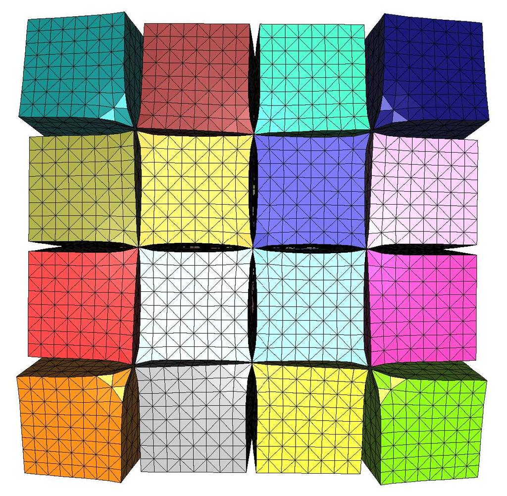
186