A robust k ε v 2 /k elliptic blending turbulence model with improved predictions in near-wall, separated and buoyant flows 1

Transcription

1 A robust ε v 2 / elliptic blending turbulence model with improved predictions in near-wall, separated and buoyant flows 1 F. Billard a,, D. Laurence a,b a School of Mechanical, Aerospace and Civil Engineering, University of Manchester, George Begg Building, Sacville Street, Manchester, M13 9PL, UK b EDF R&D MFEE, 6 quai Watier, Chatou, France Abstract This paper first reconsiders evolution over 20 years of the -epsilon-v2-f strand of eddy-viscosity models, developed since P. Durbin s 1991 original proposal for a near-wall eddy viscosity model based on the physics of the full Reynolds stress transport models, but retaining only the wall-normal fluctuating velocity variance, v2, and its source, f, the redistribution by pressure fluctuations. Added to the classical -epsilon (turbulent inetic energy and dissipation) model, this resulted in three transport equations for, epsilon and v2, and one elliptic equation for f, which accurately reproduced the parabolic decay of v2/ down to the solid wall without introducing wall-distance or low-reynolds number related damping functions in the eddy viscosity and -epsilon equations. However, most v2-f variants have suffered from numerical stiffness maing them unpractical for industrial or unsteady RANS applications, while the one version available in major commercial codes tends to lead to degraded and sometimes unrealistic solutions. After considering the rationale behind a dozen variants and asymptotic behaviour of the variables in a number of zones (balance of terms in the channel flow viscous sublayer, logarithmic layer and wae region, homogenous flows and high Reynolds number limits), a new robust version is proposed, which is also shown to yield more accurate predictions on a number of cases involving flow separation and heat transfer. This -epsilon type of model with v2/ anisotropy blends high Reynolds number and near-wall forms using two dimensionless parameters: the wall-normal anisotropy v2/ and a dimensionless parameter alpha resulting from an elliptic equation to blend the homogeneous and near-wall limiting expressions of f. The review of variants and asymptotic cases has also led to modifications of the epsilon equation: the second derivative of mean velocity is reintroduced as an extra sin term to retard turbulence growth in the transition layer (i.e. embracing the E term of the Jones and Launder (1972) -epsilon model), the homogeneous part of epsilon is now adopted as main transported variable (as it is less sensitive to the Reynolds number effects), and the excessive growth of the turbulent length-scale in the absence of production is corrected (leading to a better distinction between log layer and wae region of a channel flow). For each modification numerical stability implications are carefully considered and, after implementation in an industrial finite-volume code, the final model proved to be significantly more robust than any of the previous variants. Keywords: RANS, turbulence modelling review, channel flow buffer, logarithmic and defect layer, near-wall effects, heat transfer, unstructured finite volume method 1. Introduction The refined modelling of wall effects in the Reynolds Averaged Navier Stoes (RANS) framewor is a topic currently revitalised as Large Eddy Simulation (LES) and related hybrid RANS-LES approaches become increasingly popular and progress from low (quasi-dns) to high Reynolds wall-bounded flows. Indeed, because resolution of wall structures by LES would require very expensive meshes (of size Re 1.8, c.f. Chapman (1979)), in practice, wall turbulence is modelled using a RANS approach in the framewor of hybrid methodologies (review in Fröhlich and von Terzi (2008)). To this end, many types of near-wall RANS models have been used, from one equation to full Reynolds Stress models (RSM): to name but a few, the v 2 f model is chosen in the method of Uribe et al. (2010) whereas the PITM method of Chaouat 1 For reference update please chec here: Corresponding author. Tel: +44 (0) ; fax: +44 (0) address: flavien.billard@manchester.ac.u (F. Billard ) Preprint submitted to International Journal of Heat and Fluid Flow January 18, 2011

2 and Schiestel (2009) relies on the RSM of Launder and Shima (1989), the Elliptic Blending RSM (EBRSM) (Manceau and Hanjalić (2002)) is used in the seamless approach of Fadai-Ghotbi et al. (2010) and the (D)DES (Spalart (2009)) or the Scale Adaptive Simulation of Menter and Egorov (2005) are based on the ω SST model (Menter (1994)). Certainly the high popularity of the two latter hybrid approaches is closely related to the simplicity and robustness of the SST model, which has facilitated full scale industrial applications, e.g. complete aircrafts. Still, the latter model carries a certain amount of empiricism, as acnowledged by the author himself (Menter (1994)), and it features several empirical functions following the trend of many near-wall models (Patel et al. (1985)). Over time, and as computing power persistently grows the question as to what is the best trade-off between cost, accuracy and robustness should be revisited. The aim of the present wor is to try to devise an equivalently simple and robust approach on somehow sounder physical bases: the v 2 f model (Durbin (1991)). Its formulation inherits the minimalism of eddy viscosity models and naturally integrates wall turbulence damping by using the wall-normal fluctuations v 2 as additional scale. However it also models non-local effects of the fluctuating pressure on the turbulent fields and separately represents wall blocage effects and low Reynolds number effects. While the number of research groups focussing on RANS modelling has dwindled over the past 20 years, a notable part of the wor has been carried out in the framewor of elliptic relaxation based models, leading to several versions of the v 2 f model, which will be compared in the present article. In the first section, the pros and cons of each formulation are weighted, with focus on both stability and accuracy issues. This is followed by the presentation of the new model proposal. Lastly its performances are compared to the ω SST model and the most widely used version of the v 2 f model. The cases under consideration are two-dimensional pressure induced separating flows as well as a case of buoyancy impaired turbulence. Some three-dimensional applications are also presented. More test cases have been successfully considered, particularly for heat transfer as this is one of the areas where the original v 2 f model has been most successful, but these will be reported elsewhere: the main objective of the present paper is to propose an optimal formulation of the v 2 f type of Eddy Viscosity Model (EVM). 2. The v 2 f models 2.1. Presentation of the approach: The model stems from the standard ε system (with some low Reynolds number corrections added to the dissipation rate ε transport equation) and a third transport equation is solved for a scalar v 2, which can be assimilated near solid walls to the wall-normal fluctuations responsible for turbulent heat and momentum transfer from the wall to the core of the flow. The v 2 equation follows the classical transport equation of the wall-normal Reynolds stress component. To facilitate presentation of modelling concepts, y, v, ε 22 and φ 22 represent the wall-distance and the wall-normal component of the fluctuating velocity, the dissipation rate and the pressure-strain 2 tensors, but this does not require programming the model in a boundary fitted coordinate system as it remains at EVM level using only scalars as turbulence characterising variables. The difference between φ 22 and ε 22 is modelled as a whole (ν is the inematic molecular viscosity): φ 22 ε 22 = 2 ρ v p v v 2ν = ϕ 22 ε v2 y x x and ϕ 22 = f where f is solution of an elliptic equation: (1) f L 2 f = f h (2) L is a turbulent length-scale and f h is derived from classical second moment closure modelling in quasi homogeneous regions. In order to ensure the correct asymptotic behaviour v 2 = O(y 4 ) the following boundary condition should be used: lim f = lim 20ν 2 v 2 y 0 y 0 εy 4 (3) 2 including both pressure diffusion and redistribution. 2

3 Figure 1: A priori evaluation of the EVM relation 4 and of the standard high Reynolds turbulent viscosity expression C µ 2 /ε, compared to the exact DNS value uv/ yu for the channel flow case at Re τ = 395. Finally the model integrates v 2 in the definition of the turbulent eddy viscosity: ν t = C µ v 2 max ( ε, 6 ) ν ε (4) Durbin (1991) showed that the use of the parameter v 2 in equation 4 is the main feature allowing a correct reduction of the turbulent mixing efficiency in the buffer and viscous sublayer 3 (as seen in figure 1), circumventing the need of damping functions, à la Van Driest (1956) and subsequent models (Patel et al. (1985) review) Generic formulation of the terms and constants The definition of all models studied herein is given in the following. For a simpler comparison a generic description is adopted for the third transport equation (g = v 2 or g = v 2 /): [( D Dt = P ε + j ν + ν ) ] t j (5a) σ [( + j ν + ν ) ] t j ε (5b) Dε Dt = C ε1p C ε2 ε T Dg Dt = S g + j σ ε [( ν + ν ) t j g σ g f L 2 j j f = f h The models are referred to by the acronyms given in table 1. The terms and constants of the f, g and ε equations are given in tables 2, 3 and 4 respectively. The definitions of the length and time scales and associated constants are in table 5 and use one of the expressions 6, 7 or 8. To prevent the turbulence over-prediction at a flow stagnation point, a limiter for the turbulent time scale is proposed in Durbin (1996). The model of LIE01 proposes to use a similar limiter in the length scale for consistency. The version of T and L integrating this limiter are given in expression 8 (S represents the strain rate magnitude and is defined as S = S ij S ij with S ij = 1/2 ( i U j + j U i ) ). These limiters are effectively used in LIE01 and HAN04 models. ] (5c) (5d) 3 It may be objected that using Expression 4 yields ν t = O(y 4 ). Therefore the predicted turbulent shear stress modelled as U uv = ν t y is O(y4 ) instead of the theoretical behaviour O(y 3 ). However at walls the momentum equation budget involves the terms ν 2 U y 2 and 1 dp which are O(1). As explained in Durbin (1991) despite this inaccuracy for the wall behaviour of ρ dx the predicted turbulent shear stress, whether uv is O(y 3 ) or O(y 4 ) is insignificant. Indeed in both cases the turbulent diffusion term uv, modelled as U νt is at least two orders of magnitude smaller than the leading order terms. Liewise similar y y y arguments can be developed for the turbulent inetic energy equation. 3

4 DUR91 Durbin (1991) DUR93 Durbin (1993) DUR95 Durbin (1995) DUR96 Durbin and Laurence (1996) LIE96 Lien and Durbin (1996) PAR97 Parneix and Durbin (1997) LIE01 Lien and Kalitzin (2001) MAN02 Manceau, Carpy, and Alfano (2002b) HAN04 Hanjalić, Popovac, and Hadžiabdić (2004) URI06 Uribe (2006) Table 1: Acronyms used for models. Model f ( f h ) C 1 C 2 ϕ DUR T (C 2 1 1) 3 v2 P + C ( ) ϕ DUR T (C 2 1 1) 3 v2 P + C ( ) ϕ DUR T (C 2 1 1) 3 v2 P + C [ ( ) ] DUR96 L ϕ22 1 L T (C 2 1 1) 3 v2 P + C [ ] ϕ LIE96 22 v ε 2 T (C 1 1) 2 3 (C 1 6) v2 P + C ( ) ϕ PAR T (C 2 1 1) 3 v2 P + C [ ] ϕ LIE01 22 v ε 2 T (C 1 1) 2 3 (C 1 6) v2 P + C ( ) ϕ MAN ε εt (C 2 1 1) 3 v C 2 P ε ϕ HAN04 22 ( ) ( ) 1 P 2 T C1 1 + C 2 ε 3 v ( ) ϕ URI ν j v2 v j + ν j 2 1 j T (C 2 1 1) 3 v2 P + C ν εt v j 2 j + ν v j 2 j Table 2: Terms and coefficients of the f equation. [ L = C L max T = max L = T = [ L = C L max min [ T = max min ( ) ] 1/4, C ν 3 η ε ( ν ) ] (6) 1/2 ε 3/2 ε [ ε, C T C 2 L ( ) 3 ε + C 2 2 η ν3/2 ε 1/2 2 ε + C 2 2 T ν ε [ ] 3/2 ε, 3/2 6Cµv 2 S [ ε, 0.6 6Cµv 2 S ], C T ( ν ε, C η ( (7) ) ] 1/4 ν 3 ε ) ] (8) 1/ Evolution in the past 20 years As seen from the tables, over the last 20 years modifications mainly focussed on the numerical formulation (in search of a bettering robustness) and modelling of the wall effects in the dissipation rate equation. The original version, DUR91, used an unusually high value of the production coefficient in the ε equation (C ε1 = 1.7 instead of 1.4 as generally adopted in the RANS community). This is first corrected in DUR93, where the coefficients of the ε equation recover more traditional values in the log-layer, where P/ε = 1, together with a functional Cε1 = f(p/ε) to trigger a surge of dissipation production in the buffer layer, where P/ε > 1, with the rationale that this represents near-wall dissipation anisotropy. In DUR95 P/ε is replaced by the distance to the wall y in the definition of Cε1 to ensure the coefficient returns to its standard 4

5 Model g S g DUR91 v 2 f v 2 ε DUR93 v 2 f v 2 ε DUR95 v 2 f v 2 ε DUR96 v 2 L f v2 ε LIE96 v 2 f 6v 2 ε PAR97 v 2 f v 2 ε LIE01 v 2 f 6v 2 ε MAN02 v 2 εf v 2 ε v HAN04 2 f v2 P 2 URI06 v 2 f v2 2 P + 2 ν t v σ j 2 j Table 3: Terms and coefficients of the g equation. Note that σ g = 1.2 for HAN04. σ g = σ for all other models. Model C ε1 C ε2 σ σ ε DUR DUR ( ) 1 [ P ε ) ] 8 DUR / ( DUR ( CLy 2L ) v 2 LIE exp ( ) ( R ) y 2 PAR ( v 2 ) LIE ( v 2 ) MAN v 2 ) HAN ( v2 ( ) URI v Table 4: Terms and coefficients of the ε equation. In LIE96 R y = y /ν. Model expression for L and T C L C η C T C µ DUR91 eq DUR93 eq DUR95 eq DUR96 eq LIE96 eq PAR97 eq LIE01 eq MAN02 eq HAN04 eq URI06 eq Table 5: Lengh and time scales. 5

6 value in homogeneous cases (where P/ε > 1 and y ). Further validations proved the early proposal for Cε1 to be numerically problematic and besides, the version of DUR95 is in contradiction with the soughtafter wall-distance free property of the elliptic relaxation concept. Therefore a new parameter, /v 2, is introduced in PAR97. This latter proposal, also more consistent with near-wall dissipation anisotropy rationale, is used in all subsequent versions. Wor was also extensively performed on improving the numerical behaviour of the model. In the original version indeed, the boundary conditions for v 2 and f are coupled (equation 3) and the elliptic nature of the f equation maes the implementation very unstable in segregated codes. For the latter, the boundary condition, equation 3, requires a ratio of small terms (O(y 4 )) to be correctly computed. In practice, the time step needed to be drastically reduced. The model of LIE96 proposes to resolve the elliptic equation for the new variable f = f + 5εv 2 / 2. Doing so enables the homogeneous Dirichlet boundary condition to be used for f and therefore yields a significantly improved robustness. However LIE96 was an early model, which attempted to picup by-pass transition by a further sensitivity of Cε1 to the wall distance. The version of LIE01 combines this change of variable with the proposal of PAR97 for Cε1 and LIE01 is the version chosen by major commercial codes (StarCD, StarCCM, Fluent) for its easier convergence. HAN04 and URI06 (originally in Laurence, Uribe, and Utyuzhniov (2004)) have simultaneously and independently derived models resolving ϕ = v 2 / instead of v 2. Both teams 4 noticed a shortcoming ) in the versions of LIE96 and LIE01: the change of variable f f induces the term (5εv 2 / 2 later neglected in the f equation. However Laurence et al. (2004) shows it is of the same order as other f source terms in the logarithmic region, and its omission yields a strong over prediction of v 2. By solving this new variable ϕ, HAN04 and URI06 attempt to derive a code friendly model which, unlie LIE01, does not deteriorate the predictions of f and v 2. The derivation of the ϕ equation (equation 9) from those for v 2 and, maes a new term appear, the cross diffusion: Dϕ Dt = f P ϕ + X + j [( ) ] νt + ν j ϕ σ (9) X = 2 ν jϕ j + 2 }{{} X ν ν t σ j ϕ j } {{ } X t In HAN04 this X term is neglected and the f boundary condition is given as: (10) lim f = lim 2νϕ y 0 y 0 y 2 (11) This enhances the numerical stability because the stiffness of the boundary condition is now a ratio of O(y 2 ) terms only. However it still proved insufficiently robust for general use in a segregated industrial purpose code, and a modified version, the ζ f 0 model was derived in Popovac (2010) in the framewor of tests within the FLUENT pacage. This relies on a change of variable for f to allow a zero boundary condition for this variable, therefore this maes the ζ f 0 model inherit the same drawbacs as the models of LIE96 and LIE01. In the URI06 version the cross diffusion X term is ept in the ϕ equation and the following change of variable is proposed: f = f X ν ν j j ϕ (12) Doing so allows lim y 0 f = 0. Similarly to LIE01 a term is neglected, (X ν + ν j j ϕ), but Uribe (2006) shows it is of lesser importance. As such the formulation is numerically unstable. Indeed, in the algebraic rearrangement of the equations consecutively to the change of variable, the molecular diffusion of ϕ is cancelled in the ϕ equation, which reduces numerical stability in the viscous sub layer. In practice, ν j j ϕ is added to the ϕ source term, i.e. molecular diffusion of ϕ is effectively doubled. An undesired effect of this numerical woraround is some over-prediction of ϕ near the wall, compensated by a new tuning of the coefficients. 4 HAN04 used the letter ζ and URI06 chose ϕ. The latter notation is ept throughout this wor as a matter of consistency. 6

7 Model Re τ = 180 (Re b = 5 585) Re τ = 395 (Re b = ) Pre-print version Re τ = 590 (Re b = ) Re τ = 950 (Re b = ) Re τ = 2000 (Re b = ) DUR DUR DUR DUR LIE PAR LIE MAN HAN URI BL-v 2 / Error max Table 6: Friction coefficient C f compared to the DNS value for the same friction velocity based Reynolds number Re τ (given in %). Stepping outside the scope of numerical stability issues, we now focus on changes to the elliptic operator, equation 5d. Durbin and Laurence (1996) and Wizman et al. (1996) observe that the earlier version of the elliptic operator correctly damps the supply of v 2 in the viscous and buffer sublayers, but then erroneously augments it in the logarithmic layer, as compared to the homogeneous case, i.e: f f h, whereas f f h is needed in the logarithmic region 5. More generally, Manceau et al. (2001) shows that if the variable f behaves as y n in the log layer, the elliptic equation 5d becomes: f = f h 1 1 n(n 1)(C L κ) 2 (C µ v 2 /) 3/2 (13) f defined as ϕ22 behaves as y 1 (n = 1) in the log layer, leading to an actual amplification. The strategy adopted by DUR96 and MAN02 is to solve equation 5d for a rescaled variable f. f = Lf and f = f/ε are adopted in DUR96 and MAN02 6 respectively. These formulations leave the f variable unchanged (i.e. f = f h ) in the logarithmic region and are called neutral Behaviour in fundamental flows Using well-established DNS databases of channel flow (Kim et al. (1987), Moser et al. (1999), Alamo et al. (2004), Jimenez and Hoyas (2008)) as reference values, the sin-friction predictions of the various versions are shown in table 6 in terms of percentage. The results are mostly lying within the 10% as expected for a case used for constant tuning, but there is a clear upward (sometimes downward) drift, whence the errors are expected to increase for higher Re numbers beyond these DNS cases. In particular LIE96, PAR97, LIE01 and HAN04 models yield a maximum error ranging from 11% to 16%. The neutral formulations of DUR96 and MAN02 are clearly less affected. The properties of the logarithmic layer at infinite Reynolds number (P = ε and L = κy) are classically assumed to reduce the equations to algebraic expressions, following which the Von Kármán constant κ and anisotropy v 2 / = ϕ can be evaluated. The values returned by models in this configuration ( κ and ϕ log ) are provided in table 7, along with the value taen by the coefficient Cε1, noted Cε1,log. Behaviours of models strongly differ from one another. The Von Kármán constants predicted by LIE96 and LIE01 are excessively high and this is lined to an over prediction of ϕ log returned by the latter models. Naturally, the larger friction error drifts with Re number observed in table 6 are consistent with the larger errors on the Von Kármán constant prediction. The asymptotic values of ϕ and Cε1, in the case of homogeneous flow subject to a constant strain rate du/dy is given, table 7. Large differences amongst models can be observed. 5 with strict f < f h for purely homogeneous models or f = f h for better anisotropy reproducing high Reynolds and wall function based pressure-strain models (LRR-QI of Launder, Reece, and Rodi (1975) or SSG of Speziale, Sarar, and Gatsi (1991)). 6 MAN02 corresponds to the model presented in Manceau et al. (2002b) but this rescaled v 2 f version was originally introduced in Manceau et al. (2002a) with different values for some of the constants. 7

8 Model κ ϕ log Cε1,log ϕ Cε1, DUR DUR DUR DUR LIE PAR LIE MAN HAN URI BL-v 2 / Table 7: Predictions of the models in the logarithmic layer (left part) and in homogeneous shear turbulence (right part) Limitations of the existing versions Stability vs accuracy. Among the code-friendly formulations, none is able to effectively suppress the f boundary condition stiffness without impairing the quality of results. In LIE96 and LIE01 the terms rearrangement is done at the expense of an over prediction of v 2 in the log layer, whereas the modification proposed in URI06 leads to an overshoot of ϕ near walls. Our experience, after implementing different coding strategies, careful time-stepping and running a number of test cases is that, model version HAN04 still does not reduce the boundary condition stiffness in the f equation sufficiently. Amplification effect in the log region. All models but DUR96 and MAN02 (thans to the neutral formulation) show an overshoot of ϕ in the logarithmic layer. For LIE96 and LIE01 the combination of the two sources of over-prediction is dramatic due to a positive feedbac effect: v 2 is over-estimated due to the change of variable f f which increases the amplification factor (equation 13) which in turn increases even more v 2, and so on. Consequently those 2 models, chosen by code vendors for robustness, return values of ϕ log between 1.13 and 1.60 (table 7), which are not realisable (ϕ < 2/3). Similarly DUR95 and HAN04 return excessively high v 2 values. The inter-dependance of coefficients. In the ε model, equations 14a and 14b (Jones and Launder (1972)) determine the model behaviour in fundamental flows, where only some of the source terms of and ε are involved, and constants are tuned accordingly. Table 8 summarises the different modes. D t and Dt ε are the turbulent diffusion terms for and ε ( j (ν t /σ j ) and j (ν t /σ ε j ε) respectively). D Dt = P ε + Dt + ν j j Dε Dt = 1 T (C ε1p C ε2 ε) + Dε t + ν j j ε (14a) (14b) Mode P ε D t Dε t Constants DIT C ε2 HST C ε1 Defect Layer C ε2, σ, σ ε Log. Layer C ε1, C ε2, σ ε Near Wall C ε1, C ε2, σ, σ ε Table 8: Active and ε source terms and constants in the fundamental configurations: decaying isotropic turbulence (DIT), homogeneous shear turbulence (HST), defect layer, logarithmic layer at infinite Reynolds number and near-wall transition region. In the versions of PAR97, LIE97, LIE01, MAN02, HAN04 and URI06, the fine-tuning of ε near walls is achieved by optimising the proportionality coefficient lining C ε1 and v 2 /. However this variability subsists in the logarithmic layer and in homogeneous flows where it is undesirable. For those models, the difference in 8

9 the Cε1 definition (table 4) leads to strong diversity of prediction of the Von Kármán constant in logarithmic layer and turbulence growth rate P/ε in homogeneous shear turbulence (table 7). This interdependence also leads to a tedious calibration of the other model constants. Noteworthily the defect layer modelling (where P/ε 0) is not specifically considered in any of the formulation proposals (besides those neutralising the elliptic relaxation effect in the log-layer, which can also influence the defect layer). The wall bounded/free shear flows distinction. DUR95 is the only model able to return a substantially lower value of the coefficient C ε1 in homogeneous shear flows, hence a larger shear layer spreading rate. It is actually the difference between C ε1 and C ε2 that is most influential, but C ε2 remains fixed within each model. All other versions return the same C ε1 value regardless of the presence of a wall. 3. The present formulation A new formulation is now developed to address the problems exposed in the previous section, while simultaneously exploring more robust or code friendly solutions, which mostly stem from source terms groupings and changes of variables. One such solution was found in an adaptation to the eddy viscosity framewor of the elliptic blending RSM approach of Manceau and Hanjalić (2002). It relies on the resolution of an elliptic equation for a non-dimensional coefficient α: α L 2 j j α = 1 (15) This coefficient is given the boundary condition α = 0 at solid walls and relaxes towards 1 away from walls. It is used as a blending parameter in the v 2 source term modelling to feature a smooth transition between near-wall and quasi-homogeneous models: ϕ 22 = (1 α p ) ϕ w 22 + αp ϕ h 22. The present choice p = 3 (instead of p = 2 as in Thielen et al. (2005)) is used throughout the model s derivation following the suggestion of Lecocq (2008) who showed that a value at least equal to 3 is needed for the homogeneous term α p ϕ h 22 to vanish in the near-wall balance of the v2 transport equation. The model principal variable to be solved in a transport equation is the reduced variable ϕ = v 2 / and as such it formally can be considered as a follow-up of the wor of Laurence et al. (2004). This formulation enables setting a zero wall boundary condition for the elliptic variable α, therefore solving the numerical problems associated to the wall limit. For the definition of L and T, expression 7 is used as this provides a smoother transition between the Kolmogorov and the integral scale (Durbin and Laurence (1996)). For the coefficient C T associated to the time scale, Equation 7, the value recommended by the latter authors C T = 4 is adopted. Moreover, the constant C L is chosen so that the turbulent length-scale (Equation 7) recovers its theoretical behaviour (i.e. L = κy) in the logarithmic region in the 3/4 limit Re τ. Indeed in this situation the following holds: L = C L (C µ v /) 2 κy. Hence the value ( 3/4 C L = C µ v /) 2 = is adopted (we use the numerical value v2 / = 0.41 obtained in the logarithmic layer as presented in Table 7). Finally, similarly to HAN04, the quasi-linear SSG model has been used (but with the same simplifications as the ones performed in HAN04). However we eep here the same original values for C 1 and C 2 as recommended in Speziale et al. (1991) 7. The model uses the realisability constraint but only in the expression of the time scale present in the definition of the turbulent viscosity. This choice finds its justification in the analysis done in Sveningsson and Davidson (2004) which shows that a systematic use of the limiter wherever T is present maes it less efficient and can even lead to numerical instabilities originating from the redistribution term. The same authors also questioned the relevance of the length-scale limiter (as used in expression 8). This new proposed blended ε v 2 / model will be denoted as BL-v 2 / throughout this paper. Equations and constants of the BL-v 2 / model are given in full in Appendix A, while the incremental changes are described below: The modifications brought to the ε system can be formally seen as a double change of variable: 7 Note that the present C 2 constant is noted C 1 in their paper. 9

10 Where the E term is defined in equation 17. ε = ε h + ε E + 1 }{{} 2 ν j j (16) ε h E = 2νν t ( j U i ) ( j U i ) (17) This E term, originally proposed by Jones and Launder (1972) (JL) to account for viscous wall effects in the ε equation, is a sounder alternative to maing the production of dissipation constant Cε1 dependant on anisotropy. The E term removes some of the non-linearities and is clearly an inhomogeneity and low- Reynolds number correction (second derivative of velocity and molecular viscosity contributions respectively) which, in a channel flow maes it active only in the buffer-layer. A term by term modelling of the dissipation equation is highly debatable: ε or ω are in effect substitutes for an integral length-scale (a most essential parameter in the EVM framewor, but which does not lend itself easily to modelling at one-point transport equation level). However one may recall that the E term has much similarity with the Pε 3 term of the exact ε equation (Rodi and Mansour (1993)). Moreover the JL E term was shown to be an essential ingredient for the success in bypass transition modelling (Savill (1993), Savill (2002)). Adaptation of the E term in the framewor of v 2 f modelling was also successfully applied in the case of a sewed channel flow (Howard (1999), Howard and Sandham (2000)). However its presence introduces numerical difficulties 8. Therefore, in the present model the E term is reintroduced in the equation using the change of variable ε h = ε h + /εe. This allows it to be handled implicitly and causes no numerical instability. Moreover, the decomposition ε = ε h + 1/2ν j j is adopted from Jairlić and Hanjalić (2002) with an aim to reduce the sin term ε in the equation when 0. In the present model, a transport equation is finally solved for ε h, and to satisfy near-wall balances of the source terms in the, ε h and ϕ equations, the viscous diffusion of the three variables is halved. This also explains the presence of a factor 1/2 in the term f w of the ϕ equation. The following boundary condition is used for ε h : lim ε h = ν y 0 y 2 (18) The variable ε h is used in place of ε wherever it appears in the, ε h and ϕ equations, as well as in the definition of L and T. The formal change of variable would involve more terms which are deliberately neglected in the present approach, on the bases that they would only play a role in the vicinity of walls. Besides the numerical gain of using such a decomposition (which facilitates the numerical treatment of the E term), the latter features a decisive advantage for the model accuracy: the Kolmogorov time and length scales are used as lower bound of T and L, equations A.6, and they depend on the near-wall value of ε h. It may be argued that these Kolmogorov scales should not be influenced by the outer flow; therefore they should be independent of the Reynolds number Re τ. The variable ε h resolved by the present model is much less Re τ dependant compared to the DNS values, as shown figure 2. Indeed the presence of the term C ε3 (1 α) 3 /ε h E in the equation strongly diminishes the predicted value of the turbulent inetic energy pea in the buffer layer, the latter being nown to be strongly Re τ dependent. The sensitivity to Re τ number is mainly due to the streamwise fluctuations (and strea structures) whereas the wall-normal component v 2 is nearly independent of Re τ, therefore removing the effect of E term, via the Re τ independent ε h, on the right hand side of the ϕ equation A.4 (as well as in L and T, equations A.6) and introducing it directly into the equation A.1 is justified. Moreover, this allows an easier tuning of the model in channel flow for which case the present formulation shows the best predictions for both low and high Reynolds number, as seen on table 6. The correct theoretical behaviour of the model in the log layer is also recovered (table 7). Finally the coefficient C ε1 is ept constant, equal to its conventional value The extent of the E term effect is limited by the blending factor (1 α) 3 although the presence of the product ν ν t in E already maes it a buffer layer term. 8 It was adopted in the first version of the elliptic blending Reynolds Stress model in Manceau and Hanjalić (2002) but later abandoned (e.g. Thielen et al. (2005)). 10

11 Figure 2: Comparison of the DNS near wall dissipation rate ε (symbols) and the homogeneous dissipation rate ε h returned by the present model (symbols with solid lines) for friction velocity based Reynolds number Re τ {180; 395; 590; 950; 2000}. Figure 3: Budget of the ε equation for a channel flow, rescaled by (y + ) 2, Re τ = 395. Symbols are DNS values and lines are a priori model values. Data of Rodi and Mansour (1993). We now focus on the defect layer. The local equilibrium hypothesis P = ε characterising the logarithmic layer no longer holds further outwards. As the velocity gradient decreases turbulence is only sustained by turbulent transport terms, increasingly towards the defect layer. At the centre of the channel in the equation the equilibrium P = ε is then replaced by D T = ε, as represented in table 8 and DNS data indicate that σ = 1 is adequate. The standard values of the ε equation coefficients are calibrated to represent the logarithmic layer, homogenous shear and grid turbulence decay only. An analysis of the budget of the ε equation, as performed in Parneix et al. (1996) and also shown on figure 3 using data of Rodi and Mansour (1993), shows that if the exact ε source terms are split between rapid (P 1 +P 2 +P 3 ) and slow terms (P 4 Y ) (involving or excluding the mean velocity gradient respectively) the standard values of C ε1 = 1.44 and C ε2 = 1.83 seem overestimated by a factor two. In the logarithmic layer this overestimation is inconsequential because the excess of production and dissipation cancel each other. But even if the split between rapid and slow terms in the ε equation is highly debatable, C ε2 needs to be halved in the channel centreline region, so that it can be balanced by the turbulent transport term, which itself compares very well with the DNS data throughout the logarithmic and defect layers with the standard value of σ ε = 1.3, as shown on figure 3. Neither P/ε, nor anisotropy can be used as a criteria for reducing C ε2 in the defect layer while not affecting results in grid turbulence decay, since these parameters tae the same value in both flow configurations, hence Parneix et al. (1996) suggested a C ε2 dependency on Dε T, but in the RSM context and for the recirculation bubble in a bacstep flow. Following the same idea, a functional C ε2 is proposed here for the present model: 11

12 Figure 4: A priori evaluation of the proposed Cε2 coefficient sensitive to turbulent transport (equation 19) for a channel flow at Re τ {180; 395; 590; 950; 2000}. Figure 5: A priori evaluation of the main source term of ε, S ε = P 1 + P 2 + P 4 Y in the central region of a channel flow, Re τ = 395, influence of the use of Cε2 as defined in eq. 19. Comparison with the DNS of Mansour and Rodi (1993). C ε2 = C ε2 + α 3 (C ε4 C ε2 ) tanh ( D t ε h 3/2) (19) This results in Cε2 going from the standard value C ε2 in the logarithmic region to a decreased value of C ε4 in the defect layer. The inclusion of the blending parameter α in relation 19 is very handy as a zonal modelling parameter (rather than e.g. a turbulent Reynolds number) and ensures the Cε2 modification is not active near the wall, where turbulent transport is again significant. The a priori evaluation of Cε2 given by relation 19 for different Reynolds numbers in a channel flow is shown in figure 4. This relation yields a fairly Re τ independent characterisation of the central region of the channel. As achieved in Parneix et al. (1996), the exact source term of the ε equation is better represented using the proposed Cε2, as shown in figure 5, whereas the standard value 1.83 yields a too strongly negative ε sin term. This discrepancy of the standard model returns insufficient level of dissipation in this region resulting in a well-nown over-estimation of the turbulent viscosity and turbulent length scale (Laurence et al. (2004)). The predicted velocity and turbulent viscosity given by the model with and without using the relation 19 for Cε2 are shown in figure 6 for the channel flow case at Re τ = When using a constant Cε2 the returned turbulent viscosity is over predicted in the central region, and this discrepancy is common to all v 2 f models, and indeed a vast majority of RANS models, which lac information characterising the defect layer. This is to be directly lined to the consistent ε under-prediction. 12

13 Figure 6: Effect of Cε2 as defined in eq. 19 in a channel flow, Reτ = 2000: velocity with logarithmic scale (top) close up of the mean velocity profile with linear scale (middle) and turbulent viscosity profile (bottom). 13

14 This ν t over-prediction was shown to be especially severe for models over-predicting v 2 (for those depicting a strong amplification effect, such as the popular code-friendly version of LIE96 and LIE01, as shown in Uribe (2006)). The present version yields an improved representation of ν t in the central region, thus leading to a improved mean velocity prediction. With this modification, the model also returns the correct turbulence growth rate both in wall bounded and free shear flows. The turbulence growth P/ε now taes the different values (C ε4 1)/(C ε1 1) or (C ε2 1)/(C ε1 1) at the edge of a boundary layer and in free shear flow respectively. 4. Applications The model is validated in two classes of flows. The first type of configuration studied is two cases of pressure induced separating flows featuring a recirculation. A good prediction of the flow pattern is directly lined to the correct reproduction of the shear stress evolution, itself, in an eddy viscosity framewor, dependent on the length scale determining equation. The second category of problem under consideration is buoyancy induced turbulence generation/impairment, for which the correct near-wall turbulence damping prediction is crucial. For sae of clarity, the complete present BL-v 2 / model equations and constants, consistently benchmared on a range of test cases (Billard (2011)) is recalled in appendix A. Models are implemented in Code Saturne (Archambeau et al. (2004) and Fournier et al. (2011)) an unstructured, collocated finite volumes, time-dependent yet segregated flow solver, freely available in open-source format Pressure induced separating flows The flow through a periodically constricted channel (Almeida et al. (1993) experiment and reference LES of Temmerman and Leschziner (2001)) and in an asymmetric plane diffuser (Obi et al. (1993), Eaton (2000), reference data of Buice and Eaton (1997)) are two cases often used to validate RANS models. They are named hereafter periodic hill flow and diffuser flow. The computational domains are represented on figure 7. The length of the periodic hill domain is L 1 = 9H 1 with H 1 being the hill height. The Reynolds number based on H 1 and the bul velocity U 1 is The diffuser flow domain consists of an inlet channel of height H 2 subject to a sudden expansion with an angle of 10. The height of the outlet channel is 4.7 H 2 and the length of the computational domain is L 2 = 71H 2. The Reynolds number based on H 2 and the bul velocity U 2 is The mesh resolution is for the periodic hill flow and for the diffuser flow. In order to ensure that the present meshes are sufficiently fine, all models were run on finer meshes (with twice as many computational nodes in both directions) with no noticeable changes. Moreover the non-dimensionnal wall distance (in viscous units) of the closest cells to the wall is always smaller than unity, maing those meshes suitable for use with low Reynolds number models. The proposed BL-v 2 / version is compared to the most widely used v 2 f model of LIE01 as well as the popular ω SST model of Menter (1994). Figure 8 presents the flow pattern returned by all models on the periodic hill flow and the location of the separation and reattachment on both cases are given in table 9. Figures 9 and 11 show the sin friction prediction along the hill surface and the inclined wall of the diffuser respectively and figures 10 and 12 show the profiles of the mean stream-wise velocity and the turbulence shear stress in the two cases. In the case of the periodic hill flow relatively fair prediction of the re-circulation extent is returned by the BL-v 2 / and LIE01 models whereas the ω SST yields excessively long re-circulation. The same trend is observed on the diffuser flow. In the latter case the ω SST reattaches at the correct location but separates far too early, whereas in the hill flow it is nearly separated over the whole inter-hill region. In both flows, the recovery is slower for the ω SST model where as both v 2 f based models are in good agreement with the reference data. Those behaviours are evidenced by the mean stream-wise velocity profiles. As far as turbulent shear stress predictions are concerned, the main differences between models can be observed in the separation region of the periodic hill flow and the edge of the recirculating flow of the diffuser. The divergence between prediction of the BL-v 2 / and LIE01 models in these two configurations is relatively small despite formulations being very different, even regarding the terms and constants of the ε system on which they are based. As seen on figure 13, the C ε2 coefficient returned by the present model gradually departs from its homogeneous turbulence value of 1.83 to reach its minimum in the defect layer of 14

15 3.036H 1 y x L 1 H 1 21H 2 10 y 4.7H 2 H 2 x L 2 Figure 7: Geometry of the two pressure induced separating flows. Top: Periodic hill flow, Bottom: Diffuser flow. Periodic hill Diffuser Model Sep. Reatt. Sep. Reatt. Ref BL-v 2 / LIE ω SST Table 9: Location of the separation (Sep.) and reattachment (Reatt.) in the periodic hill flow and the diffuser flow. Distances are normalised by H 1 and H 2 respectively. the top boundary layer and most importantly just below the separation shear layer. The conventional values 1.44 and 1.83 for C ε1 and C ε2 would yield too high a turbulence growth rate therefore an under predicted recirculation size. All the v 2 f models, calibrated to return fair predictions in this type of two dimensional simple flows, use a higher value for the constant C ε1 (ranging from 1.5 to 1.55). However for all versions but DUR95 the same value is used as in homogeneous cases. On the other hand, the Cε2 modification of the present model is only activated in the presence of inhomogeneities and theoretically derived behaviours in homogeneous configurations of table 8 are properly recovered. This functional Cε2 proposal limiting the turbulence growth can be somehow compared to the turbulent viscosity limiter of the ω SST model. In the latter model, the limiter is only active when F 2 = tanh(arg2) 2 is close to 1, which is for large magnitude of the argument arg 2 defined as: arg 2 2 = max ( ωy, 500ν y 2 ω With y representing the wall distance. Liewise in the present model the constant Cε2 is decreased only in regions where the magnitude of the term D t /ε h 3/2 is the largest. Figure 14 compares the fields of D t /ε h 3/2 and arg2 2 of the respective models in the periodic hill flow. It can be seen that both terms tae their maximum values in the same regions (edge of top boundary layer and of the recirculation) indicating that the regions where the turbulence is limited by the respective models are reasonably similar 9 near the ) (20) 9 To visually emphasise the similarity between the two turbulence limiter mechanisms, a logarithmic scaling is adopted in Figure

16 LES BL-v 2 / LIE01 ω SST Figure 8: Streamlines prediction in the case of the periodic hill flow compared to the refined LES of Temmerman and Leschziner (2001). Figure 9: Prediction of the sin friction coefficient C f in the periodic hill flow. 16

17 Figure 10: Prediction of the velocity profiles (top) and the turbulence shear stress (bottom) in the periodic hill flow. Figure 9 for legends. See Figure 11: Prediction of the sin friction coefficient C f in the diffuser hill flow. See Figure 9 for legends. 17

18 Figure 12: Prediction of the velocity profiles (top) and the turbulence shear stress (bottom) in the diffuser flow. See Figure 9 for legends. Figure 13: Function C ε2 given by equation 19, returned by the BL-v2 / model in the periodic hill flow. 18

19 Figure 14: Comparison of the tanh arguments in the BL-v 2 / definition of Cε2 (i.e. SST definition of the F 2 function (bottom) (logarithmic scale). D t /ε h 3/2 ) (top) and in the ω 19

20 separation point, although further downstream the ω SST limiter seems more active than that of the present model, and this could explain why the recirculation returned by the SST model is excessively large. Noteworthily, the realisability constraint limiters present in T (for the present model) and in T and L (for the LIE01 model) do not play meaningful role in these two configurations Mixed forced and natural convection in an upward heated channel flow The added effect of buoyancy on a pressure driven fully turbulent flow was investigated in the DNS of Kasagi and Nishimura (1997) for a flow between two vertical plates ept at different temperatures, T c and T h (with T c < T h ), driven upwards by a pressure gradient (the Reynolds number based on the averaged friction velocity on the two walls and the channel half-width δ is Re τ = 150). The resulting Grashof number is Gr = , where Gr is defined as gβ(t h T c )(2δ) 3 /ν 2 (β and ν represent the volumetric expansion and the molecular viscosity respectively). The pressure gradient drives the flow upwards whereas the buoyant force drives the flow upwards (near the hot wall, aiding flow) and downwards (opposing flow). Owing to the near wall velocity profile modification by buoyancy, the turbulence is decreased in the aiding flow and increased near the opposing flow. The heat flux is modelled using a simple gradient diffusion hypothesis with a turbulent Prandtl number equal to 1. As the gravity is perpendicular to the temperature gradient, the simple model for the heat flux implies the buoyancy production is modelled as 0 in the turbulent equations. The predictions of mean velocity, mean temperature, turbulent shear stress, turbulent inetic energy and wall-normal anisotropy are shown in figure 15 for the BL-v 2 /, the LIE01 version and the ω SST model. In the buoyancy aiding side, the turbulence impairment observed is somehow captured by all models, with returned level for significantly decreased, whereas in the opposing side only the present model returns a correct level of turbulent inetic energy, and the LIE01 model yields over prediction. The ω SST consistently under predicts levels of on both sides. The near-wall anisotropy v 2 / is fairly well predicted by both v 2 f based models. The present model gives the best predictions for the turbulent shear stress therefore yielding the best velocity and temperature profiles. The relaminarisation and 50% drop of Nusselt number in the heated pipe with upward flow (buoyancy aided), You et al. (2003), is another case that the v 2 f model including the present version successfully reproduces, in opposition to an even more dramatic failure of the ω SST model. Results on this case for a selection of RANS models including an early version of the BL-v 2 / model are reported in Keshmiri et al. (2008). Other heat transfer cases (not shown here), including natural convection in a cavity (Betts and Bohari (2000)), flow in a ribbed channel (Rau et al. (1998)) and jet impinging a flat plate (Cooper et al. (1993)) were successfully run with the present model. The BL-v 2 / model was also applied to three dimensional flows: the three dimensional diffuser flow reported in Cherry et al. (2008) (the Reynolds number based on bul velocity and the inlet duct height is 10 4 ), the flow over a highly swept wing (Zhong and Turner (2009)) (the Reynolds number based on the free stream velocity and the wing chord length is ) and around the Boeing Rudimentary Landing Gear (the Reynolds number based on the free stream velocity and the wheel diameter is 10 6 )(more details on this case can be found in Spalart et al. (2010)). For the three latter cases, the simulations were run on bloc structured meshes of 1.2, 3.7 and 5.4 million cells respectively using HPC facilities. The two latter cases were run in unsteady RANS mode. Illustrative pictures of the results obtained with the present model are presented Figure 16. Conclusion A numerically robust low Reynolds number eddy viscosity model incorporating the principles of the v 2 f approach has been derived after a review of 10 variants starting from the model of Durbin (1991). The new model incorporates the near-wall turbulence damping effects through an elliptic equation but relies on the elliptic blending method originally proposed in Manceau and Hanjalić (2002) for an increased robustness. The elliptic blending approach retains the main appealing feature of the original elliptic operator 10 Switching off this constraint in the BL-v 2 / and LIE01 models increases the recirculation by a mere 1.5% and 1% respectively for the periodic hill flow. No difference is noticed in the diffuser flow. 20

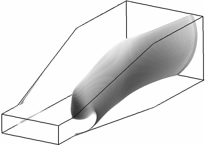
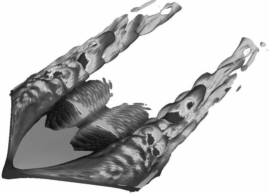
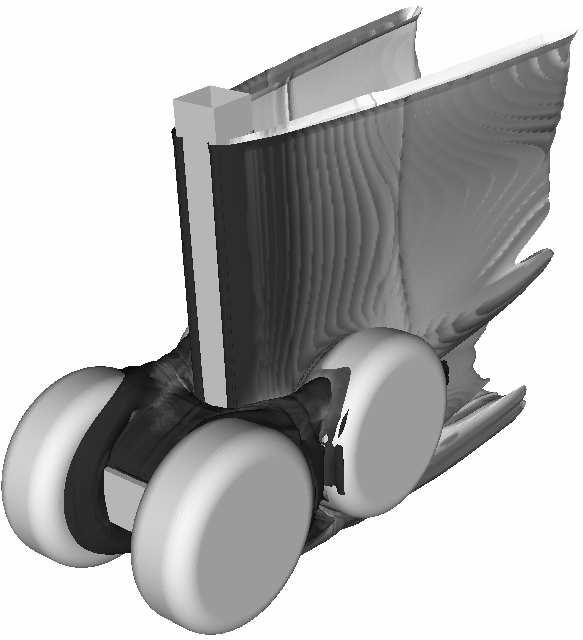
21 Figure 15: Prediction of the mean upwards velocity U +, the mean temperature T Tc T h T c, the turbulent shear-stress uv + as well as the turbulent inetic energy + and the wall-normal turbulent anisotropy v 2+ / + in the case of a flow inside a heated channel. Figure 16: Applications of the BL-v 2 / model to three-dimensional flows. Isosurface of zero streamwise velocity for the three dimensional diffuser flow and isosurface of the vorticity coloured by the turbulent inetic energy on the swept wing flow and the case of the Boeing rudimentary landing gear. 21