Transcription

1

2

3

4

5

6

7

8

9

10

11

12

13

14

15

16

17

18

19

20

21

22

23

24

25

26

27

28

29

30

31

32

33

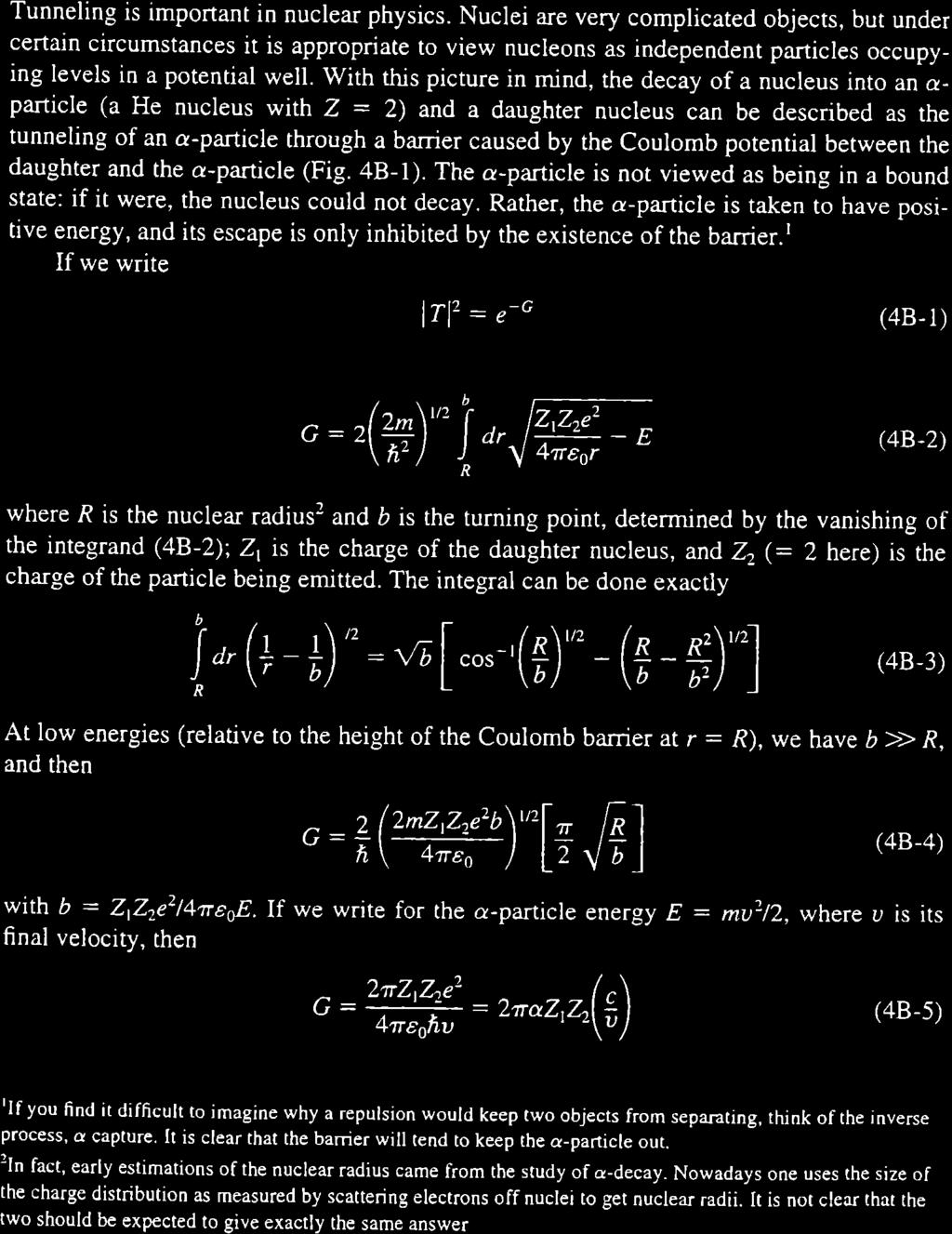
34 8.04 Quantum Physics Lecture XV One-dimensional potentials: potential step Figure I: Potential step of height V 0. The particle is incident from the left with energy E. We analyze a time independent situation where a current of particles with a welldefined energy is incident on the barrier. The time-independent SE is Ĥu(x) = Eu(x) (15-1) h 2 d 2 u (x) + V (x)u(x) = Eu(x) (15-2) 2m dx 2 d 2 u 2m dx = [E V (x)]u(x) (15-3) 2 h 2 Qualitative features of solutions for regions of constant V 1 : If E V 1 > 0, the solutions are of the form e ±ik 1x with h2 k 2 = E V 1, k 1 real. 2m Interpretation. h2 k 2 2m is the KE of the particle with total energy E in a region of potential V 1, the e ±ikx wavefunctions correspond to particles traveling left / right. Figure II: In a region where the particle energy is greater than the (constant) potential, the solutions of the SE are plane waves e ±ikx, where E V 1 = h 2 k 2 /2m is the kinetic energy of the particle in that region. If E V 1 < 0, the solutions are of the form e ±κ 1x with h2 1 2 = V 2m 1 E, κ 1 real. These are damped exponentials with a decay length constant κ 1 (decay length κ 1 1 ), where h2 κ 2 1 = V 1 E represents the missing kinetic energy of the particle 2m 1 As E V, the decay length κ 1 becomes longer and longer. κ Massachusetts Institute of Technology XV-1

35 8.04 Quantum Physics Lecture XV Figure III: In a region where the particle energy is less than the (constant) potential, the solutions of the SE are exponentially growing or decaying functions, e ±κx, where V 1 E = h 2 κ 2 /2m is the missing kinetic energy of the particle in that region. Figure IV: When a light wave experiences total internal reflection on a glass-vacuum interface, an evanescent (non-traveling, exponentially decaying wave) builds up inside the vacuum. The closer we are to the critical angle for total internal reflection, the longer the decay length of the evanescent wave. This phenomenon is analogous to a particle entering a classically forbidden region with V 1 > E. The less forbidden the region, the longer the decay length. Note. There is a non-zero probability to find the particle with energy E in a classically forbidden region with E < V 1. The less the region is forbidden (the smaller V 1 E), the further the particle penetrates into the forbidden region (the longer the decay length κ 1 1 ). The phenomenon is similar to total internal reflection inside glass at a glass-vacuum interface. The light field has non-zero amplitude in the forbidden region. How do we know? Approach with a second prism. The evanescent (decaying) field existing in the vacuum is converted back into a traveling wave in the second prism. Similarly, a particle can tunnel through a potential barrier even if its energy is insufficient to surpass it. Back to potential step Assume E > V 0 : define Massachusetts Institute of Technology XV-2

36 8.04 Quantum Physics Lecture XV Figure V: The light field tunneling through the forbidden region can be detected as it emerges on the other side in a second prism. Figure VI: As a particle tunnels through a barrier and emerges from the other side, the energy E and the Broglie wavelength 2π/k remain the same. The amplitude of the emerging wave is smaller than that of the incident wave. Figure VII: Potential step h 2 k 2 2m h 2 q 2 2m = E = E V 0 Massachusetts Institute of Technology (KE in region x < 0) (KE in region x > 0) (15-4) (15-5) XV-3

37 8.04 Quantum Physics Lecture XV The most general solution is Ae ikx + Be ikx in the region x < 0 (15-6) Ce iqx + De iqx in the region x > 0 (15-7) If we choose as the initial condition a particle incident from the left (A = 0), then the particle can be transmitted to the RHS (C = 0), or, as we shall see, partially reflected by the barrier in spite of E > V 0 (B = 0). However, if no particle is incident from the right then D = 0. Calculate the particle current (or flux) In region x < 0: ( ( ) ) h du du j < = u 2im dx u dx (15-8) h [( ) ( ) ] = A e ikx + B e ikx ikae ikx ikbe ikx c.c. 2im (15-9) hk [ ] = 2 m A 2 + AB e 2ikx A Be 2ikx B 2 c.c. (15-10) hk [ ] 2 2 = A B net current for x < 0 (15-11) m We define the reflection amplitude r = B, and the reflection coefficient as R = r 2 = A B 2. A For x > 0: hq j > = C 2 (15-12) m Continuity of wavefunction at x = 0: ψ(x 0) = A + B = ψ(x 0) = C (15-13) In spite of the potential step, the derivative of the wavefunction must also be continuous: ( ) ( ) du du ɛ d ( du ) = dx (15-14) dx x=ɛ dx x= ɛ ɛ dx 2m dx ɛ = h 2 dx[e V (x)]u(x) = 0 (15-15) For future applications, we note that if the potential contains a delta function term λδ(x a), with some magnitude of the delta function λ, then the same calculation ɛ Massachusetts Institute of Technology XV-4

38 8.04 Quantum Physics Lecture XV gives ( ) ( ) du du 2m a+ɛ = dxλδ(x a)u(λ) (15-16) dx x==a ɛ h 2 dx x=a+ɛ To summarize, we have the following rules: Rule 2.1. if the potential contains a term λδ(x a), the the first derivative du is dx discontinuous at x = a amnd satisfies the relation ( ) ( ) du du 2m = λu(a) (15-18) h 2 a ɛ Rule 1. The wavefunction u(x) is always continuous 2m = h 2 λu(a) (15-17) du Rule 2. The first spatial derivative of the wavefunction dx is continuous if the potential does not contain δ-function like terms. (It may contain potential steps). dx x=a+ɛ dx x=a ɛ Figure VIII: A discontinuity in the slope of the wavefunction occurs at a delta function potential. The difference in wavefunction slopes is proportional to the strength of the δ potential, and to the value of the wavefunction at the cusp. Continuity of ψ: A + B = C (15-19) Continuity of ψ : ik(a B) = iqc (15-20) Massachusetts Institute of Technology XV-5

39 8.04 Quantum Physics Lecture XV Solve for B, C in terms of A k C = A + B = (A B) (15-21) q ( ) ( ) k k A 1 = B 1 + (15-22) q q A q k = B q + k q q (15-23) k q B = A k + q (15-24) k q 2 C = A + B = A + A = A k + q k + q (15-25) Reflection amplitude r = B = k q (15-26) A k + q C 2k Transmission amplitude t = = (15-27) A k + q ( 2 ) 2 B k q Reflection coefficient r 2 = = (15-28) A k + q 2 C 4k 2 Transmission coefficient t 2 = A = (15-29) (k + q) 2 ( ) 2 hk Reflection current j = hk B 2 = k q A 2 (15-30) m m k + q hq 2 hk 4kq 2 Transmission current j,x>0 = C = A (15-31) m m (k + q) 2 2 Net current for x < 0 Net current for x > 0 hk hk j < = m ( A 2 B 2 ) = m 4kq A 2 (k + q) 2 (15-32) hq hk j > = m C 2 = m 4kq (k + q) 2 A 2 (15-33) The current obeys the continuity equation (see problem set) j x + t ψ 2 = 0 (15-34) Here we are considering stationary states, ψ 2 = 0 (no change of probability density t in time), = j = const, current is continuous across the potential step, j < = j >, (15-35) Massachusetts Institute of Technology XV-6

40 8.04 Quantum Physics Lecture XV or hk 2 j inc = j,x<0 = m A = j refl + j trans (15-36) = j,x<0 + j,x>0 (15-37) hk 2 hq 2 = B + C. m m (15-38) Note. r 2 + t 2 = 1 because the particle velocity is different for x < 0. x > 0 from that for Discussion of results In contrast to classical mechanics, there is some reflection at the potential step even though the energy of the particle is sufficient to surpass it. This is familiar from optics, where a step-like change in the index of refraction (e.g., air-glass interface) leads to partial reflection. The particle reflection is a consequence of the matching of the wavefunction and its derivative at the boundary. Again, this is similar to optics where the matching of th electromagnetic fields at the boundary results in a reflected field. Note. For a very smooth change of potential (or refractive index in optics) there is not reflection. What is smooth? A change over many wavelengths. Changes of the potential over a distance l short compared to a wavelength λ = 2 π result in reflection. k Slow changes of potential over many λ do not result in reflection if particle energy exceeds barrier height. Figure IX: A potential that varies smoothly over many de Broglie wavelengths does not produce partial reflection if the particle energy is sufficient to surpass it. Intermediate region l λ: we expect resonance phenomena (non-monotonic changes of reflection probability with particle energy). For the potential step, the Massachusetts Institute of Technology XV-7

41 8.04 Quantum Physics Lecture XV reflection probability 2 r 0 for k q (E V 1 ), and (15-39) 2 r 1 for q 0 (E V 1 ), as expected. (15-40) (15-41) Interestingly, the reflection probability can be written as ( ) 2 E E r 2 V1 = E + E V1 (15-42) i.e. it does not depend explicitly on h. However, the reflection is still inherenetly nonclassical in that the potential needs to change abruptly compared to the particle s de Broglie wavelength, that depends on h. Solution for E < V 0 : We define h 2k 2 = E 2m (KE for x < 0) (15-43) h 2 κ 2 = V 0 E 2m ( missing KE to surpass barrier ) (15-44) Most general solution Ae ikx + Be ikx for x < 0 (15-45) Ce κx + De κx for x > 0 (15-46) The e +κx term is not normalizable, D = 0 We can go through the same procedure as before using the continuity of ψ 1 ψ at x = 0, or use the previous calculation if we set q iκ (Ce iqx Ce κx then). Consequently, B k iκ k 2 + κ 2 r = = = = 1 (15-47) A k + iq k 2 + κ C 2k 4k 2 + κ 2 t = A = k + iκ = = 0 (15-48) k 2 + κ 2 (15-49) A part of the wave penetrates the barrier, which is why the transmission amplitude does not vanish. Note, however, that there is no associated particle current: Since Ce kx does not have a spatially varying phase, the particle current ( ) h j = ψ ψ c.c. (15-50) 2im x Massachusetts Institute of Technology XV-8

42 8.04 Quantum Physics Lecture XV vanishes for x > 0, hk 2 j < = m ( A B 2 ) = 0 (15-51) j > = 0 (15-52) The net current is zer0 in steady-state because all particles are reflected. Note. The reflected wave has an energy-dependent phase shift 2kκ with tan φ = k 2 κ 2 r = B = k iκ A k + iκ (15-53) (k iκ) 2 = k 2 + κ 2 (15-54) k 2 κ 2 2ikκ = k 2 + κ 2 (15-55) = e iφ (15-56) The phase shift of the wave is important in 3D scattering problems. Can we localize the particle in the forbidden region? Figure X: The wavefunction for E < V 0 protrudes into the forbidden region x > 0. Can the particle be observed there? To be sure that we have measured the particle inside the barrier, and not outside, we must measure its position at least with accuracy Δx κ 1. Then according to h Heisenberg uncertainty, a momentum kick exceeding Δp hκ will be trans Δx ferred onto the particle. Massachusetts Institute of Technology XV-9

43 8.04 Quantum Physics Lecture XV How much energy do we transfer? ΔE = E(p + Δp) E(p) (15-57) (p + Δp) 2 p 2 = 2m 2m (15-58) pδp (Δp) 2 = + m 2m (15-59) p = hk (15-60) pδp can be positive or negative, (Δp) 2 is always positive. the transferred energy is on average (Δp) 2 h 2 h 2κ 2 ΔE = 2m = 2m(Δx) 2 = 2m = V 0 E (15-61) According to Heisenberg uncertainty, the measurement that localizes the particle inside the barrier transfers enough energy to allow the particle to be legitimately there. Rule. A positive KE E V 1 > 0 corresponds to a spatially oscillating wavefunction e ±ikx with rate constant k (oscillation period λ = 2 π ). A negative ( missing ) KE k E V 1 < 0 corresponds to a spatially decaying or growing wavefunction e ± κx with decay rate constant κ (decay length κ 1 ). The missing KE is associated with the size of the region (κ 1 ) that the particle occupies in the classically forbidden space. Massachusetts Institute of Technology XV-10

44 8.04 Quantum Physics Lecture XVI The potential barrier: tunneling Figure I: Tunneling through a potential barrier. Assume E < V 0 (classically particle is reflected). Outside barrier solutions to the SE are u(x) = Ae ikx + Be ikx for x < a, (16-1) u(x) = Ce ikx for x > a, (16-2) (16-3) where we have omitted the term De ikx that corresponds to an incident waveform the right. Inside the barrier the SE is d 2 u 2m (x) = + (V 0 E)u(x) = κ 2 u(x) (16-4) dx 2 h 2m with κ 2 = h 2 (V o E). As before, κ is the decay constant in the classically forbidden region (κ 1 is the decay length) that is associated with the missing KE necessary to surpass the barrier classically, h2 κ 2 = V 0 E. Consequently inside the barrier 2m u(x) = Ee κx + F e κx, for x a (16-5) As before, we need to match the solution u(x) and its derivative u (x) at the boundaries. At x = a: At x = a: Ae ika + Be ika = Ee +κa + F e κa for u (16-6) +ikae ika ikbe ika = +κee +κa + κf e κa for u (16-7) Ce ika = Ee κa + F e κa for u (16-8) ikae ika = κee κa + κf e κa for u (16-9) Massachusetts Institute of Technology XVI-1

45 8.04 Quantum Physics Lecture XVI B We are interested in the reflection amplitude r = (or the reflection probability A 2 2 B C r = ) and the transmission amplitude t = (or transmission probability A A 2 C 2 t = ) from the barrier. Remember that A 2 determines the incident current, A and is a free parameter. It is useful to divide the equation for u by the equation for 1 du d u (or alternatively, match u(x) dx = dx (ln u(x)) directly. Then we write At x = a: +ikae ika ikbe +ika = κeeκa + κf e κa (16-10) Ae ika + Be ika Ee κa + F e κa At x = a: ik = +ikce ika = Ce ika κee κa + κf e κa (16-11) Ee κa + F e κa (matching of d (ln u(x)) = 1 dx u(x) dx du at boundaries). Now we proceed to eliminate E, F (Eq ): ikee κa + ikf e κa = κee κa + κf e κa (16-12) (κ + ik)ee κa = (κ ik)f e κa (16-13) E = κ ik F e 2κa (16-14) κ + ik Substitute into Eq : κ+ik RHS = κ κ ik F e 3κa + κf e κa κ ik F e 3κa + F e κ+ik κa (16-15) κ(κ ik)e +2κa + κ(κ + ik)e 2κa = (κ ik)e 2κa + (κ + ik)e 2κa (16-16) κ 2 (e 2κa e 2κa ) + ikκ(e 2κa + e 2κa ) = κ(e 2κa + e 2κa ) ik(e 2κa e 2κa ) (16-17) κ 2 sinh(2πa) + ikκ cosh(2κa) = κ cosh(2κa) ik sinh(2κa) (16-18) Massachusetts Institute of Technology XVI-2

46 8.04 Quantum Physics Lecture XVI Consequently, Eq [ ] +ikae ika ikbe ika [κ cosh(2κa) ik sinh(2κa)] (16-19) [ ] [ ] = Ae ika + Be ika κ 2 sinh(2κa) + ikκ cosh(2κa) (16-20) = Ae ika (+ikκ cosh(2κa) + k 2 sinh(2κa) + κ 2 sinh(2κa) ikκ cosh(2κa)) (16-21) = Be ika (+ikκ cosh(2κa) + k 2 sinh(2κa) κ 2 sinh(2κa) + ikκ cosh(2κa)) (16-22) [ ] [ ] Ae ika (k 2 + κ 2 ) sinh(2κa) = Be ika 2ikκ cosh(2κa) + (k 2 κ 2 ) sinh(2κa) (16-23) B r = A (16-24) (k 2 + κ 2 ) sinh(2κa) = e 2ika 2ikκ cosh(2κa) + (k 2 κ 2 ) sinh(2κa) (16-25) reflection amplitude from barrier. To calculate the transmission amplitude C, we use the continuity of u at x = a: A Ce ika = Ee κa + F e +κa (16-26) = κ ik F e κa + F e κa κ + ik (16-27) 2κ = F e κa κ + ik (16-28) Massachusetts Institute of Technology XVI-3

47 8.04 Quantum Physics Lecture XVI We find F from the continuity of u at x = a: Then, RHS = Ee κa + F e κa (16-29) = κ ik F e 3κa + F e κa (16-30) κ + ik [ ] = F e κa κ ik e 2κa + κ + ik e 2κa (16-31) κ + ik κ + ik = F e κa 2κ cosh(2κa) 2ik sinh(2κa) κ + ik (16-32) RHS = Ae ika + Be ika (16-33) = Ae ika + Ae ika (k 2 + κ 2 ) sinh(2κa) (16-34) 2ikκ cosh(2κa) + (k [ 2 κ 2 ) sinh(2κa) ] = Ae ika (k 2 + κ 2 ) sinh(2κa) 1 + (16-35) 2ikκ cosh(2κa) + (k 2 κ 2 ) sinh(2κa) 2ikκ cosh(2κa) + 2k 2 sinh(2κa) = Ae ika 2ikκ cosh(2κa) + (k 2 κ 2 ) sinh(2κa). (16-36) C 2κ F = e κa ika A A κ + ik (16-37) 2κ Ae 2ika (2ikκ cosh(2κa) + 2k 2 sinh(2κa) = A 2κ cosh(2κa) 2ik sinh(2κa) 2ikκ cosh(2κa) + (k 2 κ 2 ) sinh(2κa) (16-38) 1 = 2κe 2ika ik 2ikκ cosh(2κa) + (k 2 κ 2 ) sinh(2κa) (16-39) C = A (16-40) 2kκ = e 2ika 2kκ cosh(2κa) i(k 2 κ 2 ) sinh(2κa) (16-41) Figure II: Tunneling through the potential barrier. Consequently, we have the results for the barrier Massachusetts Institute of Technology XVI-4

48 8.04 Quantum Physics Lecture XVI h 2 k 2 2m = E h 2 κ 2 = V 2m 0 E i(k 2 +κ 2 ) sinh(2κa) B r = = e 2ika A 2kκ cosh(2κa) i(k 2 κ 2 ) sinh(2κa) t = C = e 2ika 2kκ A 2kκ cosh(2κa) i(k 2 κ 2 ) sinh(2κa) Since the energy and particle velocity are the same on both sides of the barrier, here we have r 2 + t 2 = 1. Figure III: The sinh function. Let us look at t 2 t 2 2 (2kκ) = (2kκ) 2 + (k 2 + κ2) 2 sinh 2 (2κa) (16-42) where we have used cosh 2 (x) = 1+sinh 2 (x). Since, sinh is a monotonically increasing 2m function, and κ = h 2 V0 E, the transmission is monotonically decreasing with barrier height V 0. In the limit of small transmission, κa 1 (barrier width large compared to decay ( ) 2 ( ) 2 length κ 1 1 ), we have sinh(2κa) e 2κa = 1 e 4κa and t 2 4kκ e 4κa. In this 2 4 k 2 +κ 2 limit the tunneling probability falls off exponentially with barrier thickness (in units of decay length κ 1 ). This exponential dependence explains the extremely wide variation in, e.g., lifetimes of unstable nuclei (µs to 10 9 years, corresponding to a variation by a factor of ). Massachusetts Institute of Technology XVI-5

49 8.04 Quantum Physics Lecture XVI Figure IV: The transmission through the barrier as a function of decay wavevector κ. Figure V: In the limit of large barrier height or width, the transmission falls off exponentially because the wavefunction inside the barrier is dominated by the exponentially decaying term. Potential well: resonance phenomena We first consider scattering (E > 0) x a : Ae ikx + B ikx (16-43) a x a : Ee +iqx + F e iqx (16-44) x a : Ce ikx (16-45) Figure VI: The potential well. Massachusetts Institute of Technology XVI-6

50 8.04 Quantum Physics Lecture XVI h 2 k 2 2m = E h 2 q 2 2m = V 0 + E Instead of going through the calculation again, we note that these equations are equivalent to those of the potential barrier (for E < V 0 ) if we replace κ iq. Consequently, we obtain r = ie 2ika (q 2 k 2 ) sin(2qa) 2kq cos(2qa) i(q 2 + k 2 ) sin(2qa) t = e 2ika 2kq 2kq cos(2qa) i(q 2 + k 2 ) sin(2qa) (16-46) (16-47) For the potential well, in contrast to tunneling through the barrier, the reflection and transmission oscillate as a function of parameter 2qa, i.e. as a function of number of de Broglie wavelengths 2 qπ inside the well of size a. In particular, for values 2q n a = nπ n integer (16-48) nπ q n = (16-49) 2a 2π 4a λ n = = (16-50) q n the reflection goes to zero because of destructive interference between the waves reflected at a and +a. This corresponds to the resonance condition for a Fabry-Perot resonator in optics. the phenomenon persists in 3D, and for electrons scattering off noble gas atoms is called a Ramsaner-Townsend resonance. A very similar phenomenon has been observed in collision of ultracold atoms, where the effective depth of the interatomic potential V 0 can be tuned with a magnetic field, there (and in nuclear collisions) it is called a Feshbach resonance). Bound states in attractive δ-potential What happens for negative energies V 0 < E < 0 in the potential well? We expect discrete bound states, at least if potential is sufficiently deep. Particularly simple mathematically is a limiting case where we shrink the size of the potential, simultaneously making it deeper, such that the product of depth and width is constant. Let V 0, ã 0 such that ã V 0 = const = λ > 0. We then obtain the attractive delta potential V (x) = λδ(x). We are interested in bound states: E < 0 Define h 2 κ 2 2m = 0 E = E = E, κ > 0 (16-51) Massachusetts Institute of Technology XVI-7

51 8.04 Quantum Physics Lecture XVI Figure VII: If the potential well is sufficiently deep or wide, it can support bound states with discrete energies V 0 < E < 0. Figure VIII: Attactive delta potential. Solutions for x < 0: Solutions for x > 0: Ae κx + } B{{ κx } diverges for x Ce κx + D κx (16-52) (16-53) Continuity of wavefunction at x = 0: A = D (16-54) Derivative obeys (Lecture XV) 2m u (ɛ) u ( ɛ) = h 2 λu(0) (16-55) 2m κd κa = h 2 λa (16-56) 2m 2κ = h 2 λ (16-57) Massachusetts Institute of Technology XVI-8

52 8.04 Quantum Physics Lecture XVI m κ 1 = λ (16-58) h 2 h 2κ 2 h 2 m 2 m E 1 = = h 4 λ2 = h 2 λ2 (16-59) 2m 2m 2 Binding energy for attractive δ-function. The δ potential supports Figure IX: Comparison of bound states as the potential evolves from a very deep to a very shallow potential. In the very deep potential, like in the infinite well, the wave function oscillates sinusoidally inside the well, and decays exponentially in the forbidden region. In the very shallow potential, the wavefunction is is mostly located in the forbidden region outside the well. mλ exactly one bound state of energy E = 2 2 h 2. For a finite-size well, this result corresponds to the limiting case of a weak potential that supports only one 2 h 2 mã2 bound state (V 0 mã ) with energy E = 2 h 2 V Massachusetts Institute of Technology XVI-9

53 8.04 Quantum Physics Lecture XVI Figure X: Solutions in different regions. Two attractive δ-potentials We could proceed as before, or simplify slightly by making use of the fact that the potential is symmetric x x, and therefore we expect solutions of definite parity. The even solution in the middle region is 2B cosh(κx), and A = D, which eliminates two parameters. Continuity of u: Derivative: 2B cosh(κa) = Ae κa (16-60) 2m κae κa κ2b sinh(κa) = ( ) h 2 λae κa (16-61) 2m h 2 λ κ Ae κa = 2κB sinh(κa) (16-62) ( ) 2m 2 λ κ 2B cosh(κa) = 2κB sinh(κa) (16-63) h 2ma λ 1 = tanh(κa) (16-64) h 2κa There is always exactly one solution of the eigenvalue equation (16-64) for even parity. From the figure we see that for the bound state κa < 2maλ, which is where h 2 2maλ 1 the function 1 intersects zero. On the other hand, since tanh(x) 1, we h 2 κa 1 m need 2maλ 1 < 1, or κ > λ. Larger κ means larger magnitude of binding energy κa h 2 h 2 h 2 κ 2 m 2m E = 2m. We have h 2 λ < κ < h 2 λ If we compare this to the binding-energy in m single δ-potential, κ 1 = h 2 λ we see that the particle is more strongly bound in the double-well potential. Massachusetts Institute of Technology XVI-10

54 8.04 Quantum Physics Lecture XVI Figure XI: Graphic solution of the eigenvalue equation Reason. Given the discontinuity in slope due to the potential, it is possible to choose a steeper wavefunction (larger κ larger binding energy) when the two δ-functions are close. Variation of binding energy with well separation a: As we decrease a, the Figure XII: Comparison of the wavefunction for two different well spacings. If the wells are close, for the same wavefunction discontinuity at each δ function the wavefunction outside the two wells can decay faster (larger κ), resulting in larger binding energy E = h 2 κ 2 /2m. Figure XIII: Graphic comparison of the binding energies for large and small separation 2a between the binding sites. mλ binding energy increases from the value given by κ = h 2 (binding energy of a single well attained at a ) towards the value κ = 2 mλ, attained as a 0. Thus h 2 the binding energy quadruples. the possibility of the wavefunction in a double-well system to change so as to decrease the kinetic (and possibly potential) energy is at the origin of chemical bonds in molecules. Massachusetts Institute of Technology XVI-11

55 8.04 Quantum Physics Lecture XVII For the single δ-potential we have exactly one bound state (symmetric state), for the double δ-potential we always have one symmetric bound state, and we may have (depending on the potential strength) also an antisymmetric bound state. For the finite-size potential well we may have several (but always a finite number) of bound states. Bound states in potential well Figure I: Solutions in different regions for bound states in a potential well. Here, instead of writing the solutions as exponentials, Be iqx + Ce iqx, we have already written them in a form that reflects the symmetry of the potential. We match 1 du at x = a: u dx For even solutions: C = 0 q sin(qa) κe κa = cos(qa) e κa (17-1) κ = q tan(qa) (17-2) For odd solutions: D = 0 q cos(qa) = κ sin(qa) (17-3) κ = q cot(qa) (17-4) Massachusetts Institute of Technology XVII-1

56 8.04 Quantum Physics Lecture XVII Even solutions Let us introduce y = qa, λ = 2m h 2 V 0 a 2 2ma 2 κa = h 2 E 2ma 2 = h 2 V 0 2ma2 h 2 (V 0 E ) = λ q 2 a 2 = λ y 2 (17-5) (17-6) (17-7) (17-8) Figure II: Graphic solution of the eigenvalue equation (17-2) for symmetric bound states. 2m There is always at least one solution, more if λ = h 2 V 0 a 2 is larger (potential deeper and/or wider). For λ 1, the lowest energy solutions are approximately located at ( ) h 2 2 ( ) 2 y = qa = n + 1 π, or V 0 E n = qn = h2 π 2 n + 1, similar to infinite well. 2 2m 2ma 2 2 The existence of at least one bound state is typical of 1D problems, but not of 3D problems that behave more like odd solutions. Odd solutions λ y ( π ) = cot(y) = tan + y (17-9) y 2 The looks similar to the previous plot, but with shifted RHS. For large λ, the solutions ( 2 are q n a = nσ. For small λ, a solution exists only if π ) 2 0 or 2mV 0 a π λ 2. 2 h 2 4 Massachusetts Institute of Technology XVII-2

57 8.04 Quantum Physics Lecture XVII Figure III: Graphic solution of the eigenvalue equation (17-4) for antisymmetric bound states. Figure IV: Graphic construction of an odd-state solution, or of a solution in 3D, where the wavefunction must vanish at the origin. Condition for the existence of odd solutions. In 3D, we will require that a (modified) wavefunction vanishes at the origin, therefore the solutions will look like odd-parity solutions. (It is as if the wavefunction were continued at r.) Odd solutions do not always exist because the wavefunction needs to bend around sufficiently to match a decaying exponential, this requires high KE. Figure V: If the well is not deep enough, the odd solution cannot bend down sufficiently to match (with continuous slope) a decaying exponential at the edge of the well. Massachusetts Institute of Technology XVII-3