UQ, Semester 1, 2017, Companion to STAT2201/CIVL2530 Exam Formulae and Tables

Transcription

1 UQ, Semester 1, 2017, Companion to STAT2201/CIVL2530 Exam Formulae and Tables To be provided to students with STAT2201 or CIVIL-2530 (Probability and Statistics) Exam Main exam date: Tuesday, 20 June 1

2 2

3 Probability and Monte Carlo An experiment that can result in different outcomes, even though it is repeated in the same manner every time, is called a random experiment The set of all possible outcomes of a random experiment is called the sample space of the experiment, and is denoted as Ω A sample space is discrete if it consists of a finite or countably infinite set of outcomes A sample space is continuous if it contains an interval (either finite or infinite) of real numbers, vectors or similar objects An event is a subset of the sample space of a random experiment The union of two events is the event that consists of all outcomes that are contained in either of the two events or both We denote the union as E 1 E 2 The intersection of two events is the event that consists of all outcomes that are contained in both of the two events We denote the intersection as E 1 E 2 The complement of an event in the sample space is the set of outcomes in the sample space that are not in the event We denote the complement of the event E as E The notation E c is also used Note that E E = Ω Two events, denoted E 1 and E 2 are mutually exclusive if: E 1 E 2 = where is called the empty set or null event A collection of events, E 1, E 2,, E k is said to be mutually exclusive if for all pairs, E i E j = The definition of the complement of an event implies that: (E c ) c = E The distributive law for set operations implies that (A B) C = (A C) (B C) and (A B) C = (A C) (B C) DeMorgan s laws imply that (A B) c = A c B c and (A B) c = A c B c Union and intersection are commutative operations: A B = B A and A B = B A Probability is used to quantify the likelihood, or chance, that an outcome of a random experiment will occur Whenever a sample space consists of a finite number N of possible outcomes, each equally likely, the probability of each outcome is 1/N For a discrete sample space, the probability of an event E, denoted as P (E), equals the sum of the probabilities of the outcomes in E If Ω is the sample space and E is any event in a random experiment, (1) P (Ω) = 1 (2) 0 P (E) 1 (3) For two events E 1 and E 2 with E 1 E 2 = (disjoint), P (E 1 E 2 ) = P (E 1 ) + P (E 2 ) 3

4 (4) P (E c ) = 1 P (E) (5) P ( ) = 0 The probability of event A or event B occurring is, If A and B are mutually exclusive events, P (A B) = P (A) + P (B) P (A B) P (A B) = P (A) + P (B) For a collection of mutually exclusive events, P (E 1 E 2 E k ) = P (E 1 ) + P (E 2 ) + + P (E k ) The probability of an event B under the knowledge that the outcome will be in event A is denoted P (B A) and is called the conditional probability of B given A The conditional probability of an event B given an event A, denoted as P (B A), is P (B A) = P (A B) P (A) for P (A) > 0 The multiplication rule for probabilities is: P (A B) = P (B A)P (A) = P (A B)P (B) For an event B and a collection of mutual exclusive events, E 1, E 2,, E k where their union is Ω The law of total probability yields, P (B) = P (B E 1 ) + P (B E 2 ) + + P (B E k ) = P (B E 1 )P (E 1 ) + P (B E 2 )P (E 2 ) + + P (B E k )P (E k ) Two events A and B are independent if any one of the following equivalent statements is true: (1) P (A B) = P (A) (2) P (B A) = P (B) (3) P (A B) = P (A)P (B) Observe that independent events and mutually exclusive events, are completely different concepts Don t confuse these concepts For multiple events E 1, E 2,, E n are independent if and only if for any subset of these events P (E i1 E i2 E ik ) = P (E i1 ) P (E i2 ) P (E ik ) A pseudorandom sequence is a sequence of numbers U 1, U 2, with each number, U k depending on the previous numbers U k 1, U k 2,, U 1 through a well defined functional relationship and similarly U 1 depending on the seed Ũ0 Hence for any seed, Ũ 0, the resulting sequence U 1, U 2, is fully defined and repeatable A pseudorandom sequence often lives within a discrete domain as {0, 1,, } It can then be normalised to floating point numbers with, R k = U k A good pseudorandom sequence has the following attributes among others: 1 It is quick and easy to compute the next element in the sequence 2 The sequence of numbers R 1, R 2, resembles properties as an iid sequence of uniform(0,1) random variables (iid is defined in Unit 4) Computer simulation of random experiments is called Monte Carlo and is typically carried out by setting the seed to either a reproducible value or an arbitrary value such as system time Random experiments may be replicated on a computer using Monte Carlo simulation 4

5 Distributions A random variable X is a numerical (integer, real, complex, vector, etc) summary of the outcome of the random experiment The range or support of the random variable is the set of possible values that it may take Random variables are usually denoted by capital letters A discrete random variable is an integer/real-valued random variable with a finite (or countably infinite) range A continuous random variable is a real-valued random variable with an interval (either finite or infinite) of real numbers for its range The probability distribution of a random variable X is a description of the probabilities associated with the possible values of X There are several common alternative ways to describe the probability distribution, with some differences between discrete and continuous random variables While not the most popular in practice, a unified way to describe the distribution of any scalar valued random variable X (real or integer) is the cumulative distribution function, It holds that (1) 0 F (x) 1 (2) lim x F (x) = 0 (3) lim x F (x) = 1 F (x) = P (X x) (4) If x y, then F (x) F (y) That is, F ( ) is non-decreasing Distributions are often summarised by numbers such as the mean, µ, variance, σ 2, or moments These numbers, in general do not identify the distribution, but hint at the general location, spread and shape The standard deviation of X is σ = σ 2 and is particularly useful when working with the Normal distribution Given a discrete random variable X with possible values x 1, x 2,, x n, the probability mass function of X is, p(x) = P (X = x) Note: In [MonRun2014] and many other sources, the notation used is f(x) (as a pdf of a continuous random variable) A probability mass function, p(x) satisfies: (1) p(x i ) 0 (2) p(x i ) = 1 The cumulative distribution function of a discrete random variable X, denoted as F (x), is F (x) = x i x p(x i ) P (X = x i ) can be determined from the jump at the value of x More specifically p(x i ) = P (X = x i ) = F (x i ) lim x xi F (x i ) 5

6 The mean or expected value of a discrete random variable X, is µ = E(X) = x x p(x) The expected value of h(x) for some function h( ) is: [ ] E h(x) = h(x) p(x) x The k th moment of X is, E(X k ) = x x k p(x) The variance of X, is σ 2 = V (X) = E ( (X µ) 2) = x (x µ) 2 p(x) = x x 2 p(x) µ 2 A random variable X has a discrete uniform distribution if each of the n values in its range, x 1, x 2,, x n, has equal probability Ie p(x i ) = 1/n Suppose that X is a discrete uniform random variable on the consecutive integers a, a + 1, a + 2,, b, for a b The mean and variance of X are E(X) = b + a 2 and V (X) = (b a + 1) The setting of n independent and identical Bernoulli trials is as follows: (1) There are n trials (1) The trials are independent (2) Each trial results in only two possible outcomes, labelled as success and failure (3) The probability of a success in each trial denoted as p is the same for all trials The random variable X that equals the number of trials that result in a success is a binomial random variable with parameters 0 p 1 and n = 1, 2, The probability mass function of X is ( ) n p(x) = p x (1 p) n x, x = 0, 1,, n x Useful to remember from algebra: the binomial expansion for constants a and b is (a + b) n = k=0 ( ) n a k b n k k If X is a binomial random variable with parameters p and n, then, E(X) = n p and V (X) = n p (1 p) 6

7 Given a continuous random variable X, the probability density function (pdf) is a function, f(x) such that, (1) f(x) 0 (2) f(x) = 0 for x not in the range (3) f(x) dx = 1 (4) For small x, f(x) x P (X [x, x + x)) (5) P (a X b) = b a f(x)dx = area under f(x) from a to b Given the pdf, f(x) we can get the cdf as follows: F (x) = P (X x) = x f(u)du for < x < Given the cdf of a continuous random variable, F (x) we can get the pdf: f(x) = d dx F (x) The mean or expected value of a continous random variable X, is µ = E(X) = The expected value of h(x) for some function h( ) is: [ ] E h(x) = x f(x)dx h(x)f(x) dx The k th moment of X is, E(X k ) = x k f(x) dx The variance of X, is σ 2 = V (X) = E ( (X µ) 2) = (x µ) 2 f(x)dx = x 2 f(x) dx µ 2 A continuous random variable X with probability density function f(x) = 1 b a, a x b is a continuous uniform random variable or uniform random variable for short If X is a continuous uniform random variable over a x b, the mean and variance are: µ = E(X) = a + b 2 and σ 2 = V (X) = (b a)2 12 7

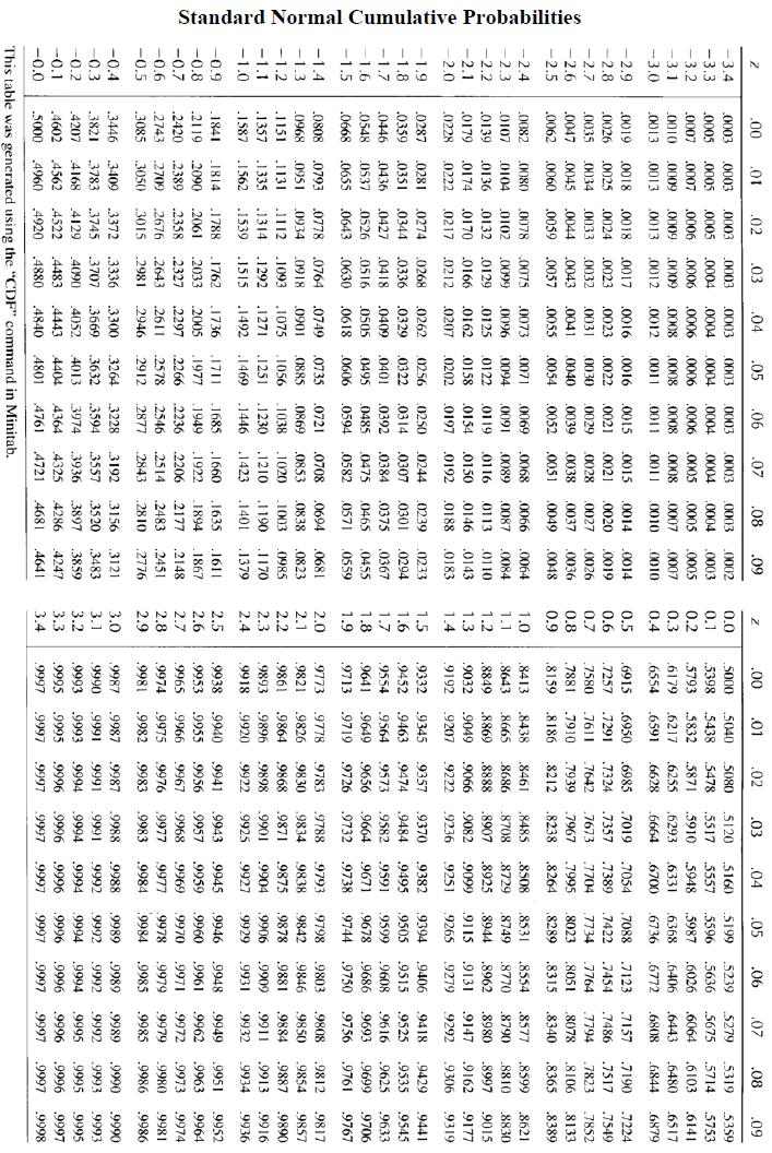
8 A random variable X with probability density function f(x) = 1 σ 2π e (x µ) 2 2σ 2, < x <, is a normal random variable with parameters µ where < µ <, and σ > 0 For this distribution, the parameters map directly to the mean and variance, E(X) = µ and V (X) = σ 2 The notation N(µ, σ 2 ) is used to denote the distribution Note that some authors and software packages use σ for the second parameter and not σ 2 A normal random variable with a mean and variance of: µ = 0 and σ 2 = 1 is called a standard normal random variable and is denoted as Z The cumulative distribution function of a standard normal random variable is denoted as and is tabulated Φ(z) = F Z (z) = P (Z z), It is very common to compute P (a < X < b) for X N(µ, σ 2 ) This is the typical way: We get: P (a < X < b) = P (a µ < X µ < b µ) ( a µ = P < X µ < b µ ) σ σ σ ( a µ = P < Z < b µ ) σ σ ( b µ ) ( a µ ) = Φ Φ σ σ ( b µ ) F X (b) F X (a) = F Z σ ( a µ ) F Z σ The exponential distribution with parameter λ > 0 is given by the survival function, F (x) = 1 F (x) = P (X > x) = e λx The random variable X that equals the distance between successive events from a Poisson process with mean number of events per unit interval λ > 0 The probability density function of X is f(x) = λe λx for 0 x < Note that sometimes a different parameterisation, θ = 1/λ is used (eg in the Julia Distributions package) The mean and variance are: µ = E(X) = 1 λ and σ 2 = V (X) = 1 λ 2 The exponential distribution is the only continuous distribution with range [0, ) exhibiting the lack of memory property For an exponential random variable X, P (X > t + s X > t) = P (X > s) Monte Carlo simulation makes use of methods to transform a uniform random variable in a manner where it follows an arbitrary given distribution One example of this is if U Uniform(0, 1) then X = 1 λ log(u) is exponentially distributed with parameter λ 8

9 Joint Probability Distributions A joint probability distribution of two random variables is also referred to as a bivariate probability distribution A joint probability mass function for discrete random variables X and Y, denoted as p XY (x, y), satisfies the following properties: (1) p XY (x, y) 0 for all x, y (2) p XY (x, y) = 0 for (x, y) not in the range (3) p XY (x, y) = 1, where the summation is over all (x, y) in the range (4) p XY (x, y) = P (X = x, Y = y) A joint probability density function for continuous random variables X and Y, denoted as f XY (x, y), satisfies the following properties: (1) f XY (x, y) 0 for all x, y (2) f XY (x, y) = 0 for (x, y) not in the range (3) f XY (x, y) dx dy = 1 (4) For small x, y: f XY (x, y) x y P (5) For any region R of two-dimensional space, ( ) P (X, Y ) R = f XY (x, y) dx dy R ( ) (X, Y ) [x, x + x) [y, y + y) A joint probability density function can also be defined for n > 2 random variables (as can be a joint probability mass function) The following needs to hold: (1) f X1 X 2 X n (x 1, x 2,, x n ) 0 (2) f X1 X 2 X n (x 1, x 2,, x n )dx 1 dx 2 dx n = 1 Most of the concepts in this section, carry over from bivariate to general multivariate distributions (n > 2) The marginal distributions of X and Y as well as the conditional distribution of X given a specific value Y = y and vice versa can be obtained from the joint distribution If the random variables X and Y are independent, then f XY (x, y) = f X (x) f Y (y) and similarly in the discrete case The expected value of a function of two random variables is: [ ] E h(x, Y ) = h(x, y)f XY (x, y) dx dy for X, Y continuous The covariance is a common measure of the relationship between two random variables (say X and Y ) It is denoted as cov(x, Y ) or σ XY, and is given by: [ ] σ XY = E (X µ X )(Y µ Y ) = E(XY ) µ X µ Y The covariance of a random variable with itself is its variance 9

10 The correlation between the random variables X and Y, denoted as ρ XY, is ρ XY = cov(x, Y ) V (X)V (Y ) = σ XY σ X σ Y For any two random variables X and Y, 1 ρ XY 1 If X and Y are independent random variables, σ XY = 0 and ρ XY = 0 The opposite case does not always hold: In general ρ XY = 0 does not imply independence But for jointly Normal random variables it does In any case, if ρ XY = 0 then the random variables are called uncorrelated When considering several random variables, it is common to consider the (symmetric) Covariance Matrix, Σ with Σ i,j = cov(x i, X j ) The probability density function of a bivariate normal distribution is 1 f XY (x, y; σ X, σ Y, µ X, µ Y, ρ) = 2πσ X σ Y 1 ρ 2 { [ ]} 1 (x µ X ) 2 exp 2(1 ρ 2 ) σx 2 2ρ(x µ X)(y µ Y ) + (y µ Y ) 2 σ X σ Y σy 2 for < x < and < y <, with parameters σ X > 0, σ Y > 0, < µ X <, < µ Y <, and 1 < ρ < 1 Given random variables X 1, X 2,, X n and constants c 1, c 2,, c n, the (scalar) linear combination (with possible affine term b), is often a random variable of interest Y = c 1 X 1 + c 2 X c n X n + b The mean of the linear combination is the linear combination of the means, E(Y ) = c 1 E(X 1 ) + c 2 E(X 2 ) + + c n E(X n ) + b This holds even if the random variables are not independent The variance of the linear combination is as follows: V (Y ) = c 2 1V (X 1 ) + c 2 2V (X 2 ) + + c 2 nv (X n ) + 2 i<j ci c j cov(x i, X j ) If X 1, X 2,, X n are independent (or even if they are just uncorrelated) V (Y ) = c 2 1V (X 1 ) + c 2 2V (X 2 ) + + c 2 nv (X n ) ( ) In case the random variables X 1,, X n were jointly Normal then, Y Normal E(Y ), V (Y ) That is, linear combinations of Normal random variables remain Normally distributed A collection of random variables, X 1,, X n is said to be iid, or independent and identically distributed if they are mutually independent and identically distributed This means that the (n - dimensional) joint probability density is a product of the individual densities In the context of statistics, a random sample is often modelled as an iid vector of random variables X 1,, X n An important linear combination associated with a random sample is the sample mean: n X = X i = 1 n n X n X n X n If X i has mean µ and variance σ 2 then sample mean (of an iid sample) has, E(X) = µ, V (X) = σ2 n 10

11 Descriptive Statistics Descriptive statistics deals with summarizing data using numbers, qualitative summaries, tables and graphs Here are some types of data configurations: 1 Single sample: x 1, x 2,, x n 2 Single sample over time (time series): x t1, x t2,, x tn with t 1 < t 2 < < t n 3 Two samples: x 1,, x n and y 1,, y m 4 Generalizations from two samples to k samples (each of potentially different sample size, n 1,, n k ) 5 Observations in tuples: (x 1, y 1 ), (x 2, y 2 ),, (x n, y n ) 6 Generalizations from tuples to vector observations (each vector of length l), (x 1 1,, x l 1),, (x 1 n,, x l n) Individual variables may be categorical or numerical Categorical variables (taking values in one of several categories) may be ordinal meaning that they can be sorted (eg low, moderate, high ), or not (eg cat, dog, fish ) A statistic is a quantity computed from a sample (assume here a single sample x 1,, x n ) Here are very common and useful statistics: 1 The sample mean: x = x x n = n n (x i x) 2 x 2 i n x2 2 The sample variance: s 2 = = n 1 n 1 3 The sample standard deviation: s = s 2 4 Order statistics work as follows: Sort the sample to obtain the sequence of sorted observations, denoted x (1),, x (n) where, x (1) x (2) x (n) Some common order statistics: (a) The minimum min(x 1,, x n ) = x (1) (b) The maximum max(x 1,, x n ) = x (n) (c) The median median = { x( n x i ( x( n 2 ) + x ( n 2 +1) ) 2 ) if n is odd, if n is even Note that the median is the 50 th percentile and the 2nd quartile (see below) (d) The q th quantile (q [0, 1]) or alternatively the p = 100q percentile (measured in percents instead of a decimal), is the observation such that p percent of the observations are less than it and (1 p) percent of the observations are greater than it In cases (as is typical) that there is not such a precise observation, it is a linear interpolation between two neighbouring observations (as is done for the median when n is even) In terms of order statistics, the q th quantile is approximately (not taking linear interpolations into account) x ([q n]) Here [z] denotes the nearest integer in {1,, n} to z (e) The first quartile, denoted Q1 is the 25th percentile The second quartile (Q2) is the median The third quartile, denoted Q3 is the 75th percentile Thus half of the observations lie between Q1 and Q3 In other words, the quartiles break the sample into 4 quarters The difference Q3 Q1 is the interquartile range (f) The sample range is x (n) x (1) 11

12 Constructing a Histogram (Equal Bin Widths) (1) Label the bin (class interval) boundaries on a horizontal scale (2) Mark and label the vertical scale with frequencies or counts (3) Above each bin, draw a rectangle where height is equal to the frequency (or count) A Kernel Density Estimate (KDE) is a way to construct a Smoothed Histogram While construction is not as straightforward as steps (1) (3) above, automated tools can be used Both the histogram and the KDE are not unique in the way they summarize data With these methods, different settings (eg number of bins in histograms or bandwidth in a KDE) may yield different representations of the same data set Nevertheless, they are both very common, sensible and useful visualisations of data The box plot is a graphical display that simultaneously describes several important features of a data set, such as centre, spread, departure from symmetry, and identification of unusual observations or outliers It is often common to plot several box plots next to each other for comparison An anachronistic, but useful way for summarising small data-sets is the stem and leaf diagram In a cumulative frequency plot the height of each bar is the total number of observations that are less than or equal to the upper limit of the bin The Empirical Cumulative Distribution Function (ECDF) is, ˆF (x) = 1 n 1{x i x} Here 1{ } is the indicator function The ECDF is a function of the data, defined for all x Given a candidate distribution with cdf F (x), a probability plot is a plot of the ECDF (or sometimes just it s jump points) with the y-axis stretched by the inverse of the cdf F 1 ( ) The monotonic transformation of the y-axis is such that if the data comes from the candidate F (x), the points would appear to lie on a straight line Names of variations of probability plots are the P-P plot and Q-Q plot (these plots are similar to the probability plot) A very common probability plot is the Normal probability plot where the candidate distribution is taken to be Normal(x, s 2 ) The Normal probability plot can be useful in identifying distributions that are symmetric but that have tails that are heavier or lighter than the Normal A time series plot is a graph in which the vertical axis denotes the observed value of the variable and the horizontal axis denotes time A scatter diagram is constructed by plotting each pair of observations with one measurement in the pair on the vertical axis of the graph and the other measurement in the pair on the horizontal axis The sample correlation coefficient r xy is an estimate for the correlation coefficient, ρ, presented in the previous unit: (y i y)(x i x) r xy = (y i y) 2 (x i x) 2 12

13 Statistical Inference Ideas Statistical Inference is the process of forming judgements about the parameters of a population, typically on the basis of random sampling The random variables X 1, X 2,, X n are an (iid) random sample of size n if (a) the X i s are independent random variables and (b) every X i has the same probability distribution A statistic is any function of the observations in a random sample, and the probability distribution of a statistic is called the sampling distribution Any function of the observation, or any statistic, is also a random variable We call the probability distribution of a statistic a sampling distribution A point estimate of some population parameter θ is a single numerical value ˆθ of a statistic ˆΘ The statistic ˆΘ is called the point estimator The most common statistic we consider is the sample mean, X, with a given value denoted by x As an estimator, the sample mean is an estimator of the population mean, µ Central Limit Theorem (for sample means): If X 1, X 2,, X n is a random sample of size n taken from a population with mean µ and finite variance σ 2 and if X is the sample mean, the limiting form of the distribution of as n, is the standard normal distribution Z = X µ σ/ n This implies that X is approximately normally distributed with mean µ and standard deviation σ/ n The standard error of X is given by σ/ n In most practical situations σ is not known but rather estimated in this case, the estimated standard error, (denoted in typical computer output as SE ), is s/ n where s is the point estimator, x 2 i n x2 s = n 1 Central Limit Theorem (for sums): Manipulate the central limit theorem (for sample means and use n Z = n X i n µ, nσ 2 which follows a standard normal distribution as n X i = nx This yields, This implies that n X i is approximately normally distributed with mean n µ and variance n σ 2 Knowing the sampling distribution (or the approximate sampling distribution) of a statistic is the key for the two main tools of statistical inference that we study: (a) Confidence intervals a method for yielding error bounds on point estimates (b) Hypothesis testing a methodology for making conclusions about population parameters 13

14 The formulas for most of the statistical procedures use quantiles of the sampling distribution When the distribution is N(0, 1) (standard normal), the α quantile is denoted z α and satisfies: zα 1 α = e x2 2 dx 2π A common value to use for α is 005 and in procedures the expressions z 1 α or z 1 α/2 appear Note that in this case z 1 α/2 = A confidence interval estimate for µ is an interval of the form l µ u, where the end-points l and u are computed from the sample data Because different samples will produce different values of l and u, these end points are values of random variables L and U, respectively Suppose that P ( L µ U ) = 1 α The resulting confidence interval for µ is l µ u The end-points or bounds l and u are called the lower- and upper-confidence limits (bounds), respectively, and 1 α is called the confidence level If x is the sample mean of a random sample of size n from a normal population with known variance σ 2, a 100(1 α)% confidence interval on µ is given by x z 1 α/2 σ n µ x + z 1 α/2 σ n Note that it is roughly of the form, x 2 SE(x) µ x + 2 SE(x) Confidence interval formulas give insight into the required sample size: If x is used as an estimate of µ, we can be 100(1 α)% confident that the error x µ will not exceed a specified amount when the sample size is not smaller than ( ) z1 α/2 σ 2 n = A statistical hypothesis is a statement about the parameters of one or more populations The null hypothesis, denoted H 0 is the claim that is initially assumed to be true based on previous knowledge The alternative hypothesis, denoted H 1 is a claim that contradicts the null hypothesis For some arbitrary value µ 0, a two-sided alternative hypothesis would be expressed as follows: H 0 : µ = µ 0 H 1 : µ µ 0, whereas a one-sided alternative hypothesis would be expressed as: H 0 : µ = µ 0 H 1 : µ < µ 0 or H 0 : µ = µ 0 H 1 : µ > µ 0 The standard scientific research use of hypothesis is to hope to reject H 0 so as to have statistical evidence for the validity of H 1 An hypothesis test is based on a decision rule that is a function of the test statistic For example: Reject H 0 if the test statistic is below a specified threshold, otherwise don t reject 14

15 Rejecting the null hypothesis H 0 when it is true is defined as a type I error Failing to reject the null hypothesis H 0 when it is false is defined as a type II error H 0 Is True H 0 Is False Fail to reject H 0 : No error Type II error Reject H 0 : Type I error No error α = P (type I error) = P (reject H 0 H 0 is true) β = P (type II error) = P (fail to reject H 0 H 0 is false) The power of a statistical test is the probability of rejecting the null hypothesis H 0 when the alternative hypothesis is true A typical example of a simple hypothesis test has H 0 : µ = µ 0 vs H 1 : µ = µ 1, where µ 0 and µ 1 are some specified values for the population mean This test isn t typically practical but is useful for understanding the concepts at hand Assuming that µ 0 < µ 1 and setting a threshold, τ, reject H 0 if the x > τ, otherwise don t reject Explicit calculation of the relationships of τ, α, β, n, σ, µ 0 and µ 1 is possible in this case In most hypothesis tests used in practice (and in this course), a specified level of type I error, α is predetermined (eg α = 005) and the type II error is not directly specified The probability of making a type II error β increases (power decreases) rapidly as the true value of µ approaches the hypothesized value The probability of making a type II error also depends on the sample size n - increasing the sample size results in a decrease in the probability of a type II error The population (or natural) variability (eg described by σ) also affects the power The P -value is the smallest level of significance that would lead to rejection of the null hypothesis H 0 with the given data That is, the P -value is based on the data It is computed by considering the location of the test statistic under the sampling distribution based on H 0 It can also be viewed as the probability of observing a set of data which is as consistent or more consistent with the alternative hypothesis than the observed data, when the null hypothesis is true It is customary to consider the test statistic (and the data) significant when the null hypothesis H 0 is rejected; therefore, we may think of the P -value as the smallest α at which the data are significant In other words, the P -value is the observed significance level Clearly, the P -value provides a measure of the credibility of the null hypothesis Computing the exact P -value for a statistical test is not always doable by hand It is typical to report the P -value in studies where H 0 was rejected (and new scientific claims were made) Typical ( convincing ) values can be of the order 0001 A General Procedure for Hypothesis Tests is (1) Parameter of interest: From the problem context, identify the parameter of interest (2) Null hypothesis, H 0 : State the null hypothesis, H 0 (3) Alternative hypothesis, H 1 : Specify an appropriate alternative hypothesis, H 1 (4) Test statistic: Determine an appropriate test statistic (5) Reject H 0 if: State the rejection criteria for the null hypothesis (6) Computations: Compute any necessary sample quantities, substitute these into the equation for the test statistic, and compute the value (7) Draw conclusions: Decide whether or not H 0 should be rejected and report that in the problem context 15

16 Single Sample Inference The setup is a sample x 1,, x n (collected values) modelled by an iid sequence of random variables, X 1,, X n The parameter at question in this unit is the population mean, µ = E[X i ] A point estimate is x (described by the random variable X) We devise hypothesis tests and confidence intervals for µ, distinguishing between the (unrealistic but simpler) case where the population variance, σ 2, is known, and the more realistic case where it is not known and estimated by the sample variance, s 2 For very small samples, the results we present are valid only if the population is normally distributed But for non-small samples (eg n > 20, although there isn t a clear rule), the central limit theorem provides a good approximation and the results are approximately correct Testing Hypotheses on the Mean, Variance Known (Z-Tests) iid Model: X i N(µ, σ 2 ) with µ unknown but σ 2 known Null hypothesis: H 0 : µ = µ 0 Test statistic: z = x µ 0 σ/ n, Z = X µ 0 σ/ n Alternative P -value Rejection Criterion Hypotheses for Fixed-Level Tests H 1 : µ µ 0 P = 2 [ 1 Φ ( z )] z > z 1 α/2 or z < z α/2 H 1 : µ > µ 0 P = 1 Φ ( z ) z > z 1 α H 1 : µ < µ 0 P = Φ ( z ) z < z α Note: For H 1 : µ µ 0, a procedure identical to the preceding fixed significance level test is: Reject H 0 : µ = µ 0 if either x < a or x > b where a = µ 0 z 1 α/2 σ n and b = µ 0 + z 1 α/2 σ n Compare these results with the confidence interval formula (presented in previous unit): x z 1 α/2 σ n µ x + z 1 α/2 σ n In this case, if H 0 is not true and H 1 holds with a specific value of µ = µ 1, then it is possible to compute the probability of type II error, β In the (very realistic) case where σ 2 is not known, but rather estimated by S 2, we would like to replace the test statistic, Z, above with, T = X µ 0 S/ n, but in general, T no longer follows a Normal distribution Under H 0 : µ = µ 0, and for moderate or large samples (eg n > 100) this statistic is approximately Normally distributed just like above In this case, the procedures above work well 16

17 But for smaller samples, the distribution of T is no longer Normally distributed Nevertheless, it follows a well known and very famous distribution of classical statistics: The Student-t Distribution The probability density function of a Student-t Distribution with a parameter v, referred to as degrees of freedom, is, f(x ; v) = Γ[ (v + 1)/2 ] πvγ(v/2) 1 [ (x 2 /v ) + 1] (v+1)/2 < x <, where Γ( ) is the Gamma-function It is a symmetric distribution about 0 and as v it approaches a standard Normal distribution The following mathematical result makes the t-distribution useful: Let X 1, X 2,, X n be an iid sample from a Normal distribution with mean µ and variance σ 2 The random variable, T has a t-distribution with n 1 degrees of freedom Now, knowing the distribution of T (and noticing it depends on the sample size, n), allows us to construct hypothesis tests and confidence intervals when σ 2 is not known, analogous to the (Z-tests and confidence intervals) presented above If x and s are the mean and standard deviation of a random sample from a normal distribution with unknown variance σ 2, a 100(1 α)% confidence interval on µ is given by s s x t 1 α/2,n 1 µ x + t n 1 α/2,n 1, n where t 1 α/2,n 1 is the 1 α/2 quantile of the t distribution with n 1 degrees of freedom A related concept is a 100(1 α)% prediction interval (PI) on a single future observation from a normal distribution is given by x t 1 α/2,n 1 s n X n+1 x + t 1 α/2,n 1 s n This is the range where we expect the n + 1 observation to be, after observing n observations and computing x and s Testing Hypotheses on the Mean, Variance Unknown (T-Tests) iid Model: X i N(µ, σ 2 ) with both µ and σ 2 unknown Null hypothesis: H 0 : µ = µ 0 Test statistic: t = x µ 0 s/ n, T = X µ 0 S/ n Alternative P -value Rejection Criterion Hypotheses for Fixed-Level Tests H 1 : µ µ 0 P = 2 [ ( )] 1 F n 1 t t > t 1 α/2,n 1 or t < t α/2,n 1 H 1 : µ > µ 0 P = 1 F n 1 ( t ) H 1 : µ < µ 0 P = F n 1 ( t ) t > t 1 α,n 1 t < t α,n 1 Note that here, F n 1 ( ) denotes the cdf of the t-distribution with n 1 degrees of freedom As opposed to Φ( ), it is not tabulated in standard tables and like Φ( ) it cannot be explicitly evaluated So to calculate P -values, we use software 17

18 Two Sample Inference The setup is a sample x 1,, x n1 modelled by an iid sequence of random variables, X 1,, X n1 and another sample y 1,, y n2 modelled by an iid sequence of random variables, Y 1,, Y n1 Observations, x i and y i (for same i) are not paired In fact, it is possible that n 1 n 2 (unequal sample sizes) iid The model assumed is, X i N(µ 1, σ1 2), Y iid i N(µ 2, σ2 2) Variations are: (i) equal variances: σ1 2 = σ2 2 := σ2 (ii) unequal variances: σ2 2 σ2 2 We could carry single sample inference for each population separately Specifically, for µ 1 = E[X i ] and µ 2 = E[Y i ] However we focus on, µ := µ 1 µ 2 = E[X i ] E[Y i ] For this difference in means we can carry out inference jointly It is very common to ask if µ (=, <, >) 0, ie if µ 1 (=, <, >) µ 2 But we can also replace the 0 with other values, eg µ 1 µ 2 = 0 for some 0 A point estimator for µ is X Y (difference in sample means) The estimate from the data is denoted by x y (the difference in the individual sample means), with, x = 1 n 1 x i, y = 1 n 2 y i n 1 n 2 In the case (ii) of unequal variances: Point estimates for σ1 2 and σ2 2 are the individual sample variances, s 2 1 = 1 n 1 (x i x) 2, s 2 2 = 1 n 2 (y i y) 2 n 1 1 n 2 1 In case (i) of equal variances, both S 2 1 and S2 2 estimate σ2 In this case, a more reliable estimate can be obtained via the pooled variance estimator Sp 2 = (n 1 1)S1 2 + (n 2 1)S2 2 n 1 + n 2 2 In case (i), under H 0 : T = X Y 0 ( 1 S p + 1 t n1 + n 2 2 ) n 1 n 2 That is, the T test statistic follows a t-distribution with n 1 + n 2 2 degrees of freedom In case (ii), under H 0, there is only the approximate distribution, where the degrees of freedom are T = X Y 0 S1 2 + S2 2 n 1 n 2 v = ( s 2 1 n 1 + s2 2 ( ) 2 s 2 1 /n 1 n approx t ( v ) n 2 ) 2 ( s 2 2 /n 2 n 2 1 If v is not an integer, may round down to the nearest integer (for using a table) ) 2 18

19 Case (i): Testing Hypotheses on Differences of Mean, Variance Unknown and Assumed Equal (two sample T-Tests with equal variance) iid Model: X i N(µ 1, σ 2 iid ), Y i N(µ 2, σ 2 ) Null hypothesis: H 0 : µ 1 µ 2 = 0 Test statistic: t = x y 0 s p 1 n n 2, T = X Y 0 S p 1 n n 2 Alternative P -value Rejection Criterion Hypotheses for Fixed-Level Tests H 1 : µ 1 µ 2 0 P = 2 [ ( )] 1 F n1 +n 2 2 t H 1 : µ 1 µ 2 > 0 H 1 : µ 1 µ 2 < 0 ( ) P = 1 F n1 +n 2 2 t ( ) P = F n1 +n 2 2 t t > t 1 α/2,n1 +n 2 2 or t < t α/2,n1 +n 2 2 t > t 1 α,n1 +n 2 2 t < t α,n1 +n 2 2 Case (ii): Testing Hypotheses on Differences of Mean, Variance Unknown and NOT Equal (two sample T-Tests with unequal variance) Model: X i iid N(µ 1, σ 2 1 ), Y i Null hypothesis: H 0 : µ 1 µ 2 = 0 Test statistic: t = x y 0 S 2 1 n 1 + S2 2 n 2 iid N(µ 2, σ 2 2 ), T = X Y 0 S 2 1 n 1 + S2 2 n 2 Alternative P -value Rejection Criterion Hypotheses for Fixed-Level Tests H 1 : µ 1 µ 2 0 P = 2 [ ( )] 1 F v t t > t 1 α/2,v or t < t α/2,v H 1 : µ 1 µ 2 > 0 P = 1 F v ( t ) H 1 : µ 1 µ 2 < 0 P = F v ( t ) t > t 1 α,v t < t α,v Case (i) (Equal variances) - confidence interval: x y t 1 α/2,n1 +n 2 2 s p 1 n n 2 µ 1 µ 2 x y + t 1 α/2,n1 +n 2 2 s p 1 n n 2 Case (ii) (NOT Equal variances) - confidence interval: s 2 1 x y t α/2,v + s2 2 s 2 1 µ 1 µ 2 x y + t n 1 n α/2,v + s2 2 2 n 1 n 2 19

20 Linear Regression The collection of statistical tools that are used to model and explore relationships between variables that are related in a nondeterministic manner is called regression analysis Of key importance is the conditional expectation, E(Y x) = µ Y x = β 0 + β 1 x with Y = β 0 + β 1 x + ɛ, where x is not random and ɛ is a Normal random variable with E(ɛ) = 0 and V (ɛ) = σ 2 Simple Linear Regression is the case where both x and y are scalars, in which case the data is, (x 1, y 1 ),, (x n, y n ) Then given estimates of β 0 and β 1 denoted by ˆβ 0 and ˆβ 1 we have y i = ˆβ 0 + ˆβ 1 x i + e i i = 1, 2,, n, where e i, are the residuals and we can also define the predicted observation, ŷ i = ˆβ 0 + ˆβ 1 x i Ideally it would hold that y i = ŷ i (e i = 0) and thus total mean squared error L := SS E = e 2 i = (y i ŷ i ) 2 = (y i ˆβ 0 ˆβ 1 x i ) 2, would be zero But in practice, unless σ 2 = 0 (and all points lie on the same line), we have that L > 0 The standard (classic) way of determining the statistics ( ˆβ 0, ˆβ 1 ) is by minimisation of L The solution, called the least squares estimators must satisfy L = 2 (y i β ˆβ 0 ˆβ 1 x i ) = 0 0 ˆβ0 ˆβ1 L β 1 ˆβ0 ˆβ1 = 2 Simplifying these two equations yields n ˆβ 0 + ˆβ 1 ˆβ 0 (y i ˆβ 0 ˆβ 1 x i )x i = 0 x i = x i + ˆβ 1 y i x 2 i = y i x i These are called the least squares normal equations The solution to the normal equations results in the least squares estimators ˆβ 0 and ˆβ 1 Using the sample means, x and y the estimators are, ( ) y i)( x i y i x i ˆβ 0 = y ˆβ n 1 x, ˆβ1 = ( ) 2 x i x 2 i n 20

21 The following quantities are also of common use: Hence, Further, S xy = S xx = (x i x) 2 = (y i y)(x i x) = x 2 i x i y i ˆβ 1 = S xy S xx ( ) 2 x i n ( i)( ) x y i n SS T = (y i y) 2, SS R = (ŷ i y) 2, SS E = (y i ŷ i ) 2 The Analysis of Variance Identity is or, Also, SS R = ˆβ 1 S xy ( ) 2 ( ) 2 ) 2 y i y = ŷ i y + (y i ŷ i SS T = SS R + SS E An Estimator of the Variance, σ 2 is ˆσ 2 := MS E = SS E n 2 A widely used measure for a regression model is the following ratio of sum of squares, which is often used to judge the adequacy of a regression model: R 2 = SS R SS T = 1 SS E SS T ( ) ( ) E ˆβ0 = β 0, V ˆβ0 = σ 2 [ 1 n + x2 S XX ( ) ( ) E ˆβ1 = β 1, V ˆβ1 = σ2 S XX In simple linear regression, the estimated standard error of the slope and the estimated standard error of the intercept are ( ) ˆσ 2 ( ) [ ] 1 se ˆβ1 = and se ˆβ0 = ˆσ 2 S XX n + x2 ] S XX 21

22 The Test Statistic for the Slope is T = ˆβ 1 β 1,0 ˆσ 2 /S XX H 0 : β 1 = β 1,0 H 1 : β 1 β 1,0 Under H 0 the test statistic T follows a t - distribution with n 2 degree of freedom An alternative is to use the F statistic as is common in ANOVA (Analysis of Variance) not covered fully in the course SS R /1 F = SS E /(n 2) = MS R MS E Under H 0 the test statistic F follows an F - distribution with 1 degree of freedom in the numerator and n 2 degrees of freedom in the denominator Analysis of Variance Table for Testing Significance of Regression Source of Sum of Degrees of Mean F 0 Variation Squares Freedom Square Regression SS R = ˆβ 1 S xy 1 MS R MS R /MS E Error SS E = SS T ˆβ 1 S xy n 2 MS E Total SS T n 1 There are also confidence intervals for β 0 and β 1 as well as prediction intervals for observations We don t cover these formulas To check the regression model assumptions we plot the residuals e i and check for (i) Normality (ii) Constant variance (iii) Independence Logistic Regression: Take the response variable, Y i as a Bernoulli random variable In this case notice that E(Y ) = P (Y = 1) The logit response function has the form ( ) E Y = exp(β 0 + β 1 x) ( ) 1 + exp β 0 + β 1 x Fitting a logistic regression model to data yields estimates of β 0 and β 1 The following formula is called the odds ( ) E Y ( ) ( ) = exp β 0 + β 1 x 1 E Y 22

23 23

24 24