6 Source Characterization

Transcription

1 6 Source Characterization Source characterization describes the rate at which earthquakes of a given magnitude, and dimensions (length and width) occur at a given location. For each seismic source, the source characterization develops a suite of credible and relevant earthquake scenarios (magnitude, dimension, and location) and computes the rate at which each earthquake scenario occurs. The first step in the source characterization is to develop a model of the geometry of the sources. There are two basic approaches used to model geometries of seismic sources in hazard analyses: areal source zone and faults sources. Once the source geometry has been modelled, then models are then developed to describe the occurrence of earthquakes on the source. This includes models that describe the distribution of earthquake magnitudes, the distribution of rupture dimensions for each earthquake magnitude, the distribution of locations of the earthquakes for each rupture dimension, and the rate at which earthquakes occur on the source (above some minimum magnitude of interest). 6.1 Geometrical Models Used for Seismic Sources in Hazard Analyses In the 1970s and early 1980s, the seismic source characterization was typically based on historical seismicity data using seismic zones (called areal sources). In many parts of the world, particularly those without known faults, this is still the standard of practice. In regions with geologic information on the faults (slip-rates or recurrence intervals), the geologic information can be used to define the activity rates of faults Areal Source Zones Areal source zones are used to model the spatial distribution of seismicity in regions with unknown fault locations. In general, the areal source zone is a volume; there is a range on the depths of the seismicity in addition to the plot of the zone in map view. 6-1

2 Even for regions with known faults, background zones modeled as areal sources are commonly included in the source characterization to account for earthquakes that occur off of the known faults. Gridded seismicity is another type of areal source. In this model the dimensions of the areal source zones are small. The seismicity rate for each small zone is not based solely on the historical seismicity that has occurred in the small zone, but rather it is based on the smoothed seismicity smoothed over a much larger region. This method of smoothed seismicity has been used by the USGS in the development of national hazard maps (e.g. Frankel et al, 1996) Fault Sources Fault sources were initially modelled as multi-linear line sources. Now they are more commonly modelled as multi-planar features. The earthquake ruptures are distributed over the fault plane. Usually, the rupture are uniformly distributed along the fault strike, but may have a non-uniform distribution along strike. 6.2 Seismic moment, moment magnitude, and stress-drop We begin with some important equations in seismology that provide a theoretical basis for the source scaling relations. The seismic moment, M o (in dyne-cm), of an earthquake is given by M o = µ A D (6.1) where µ is the shear modulus of the crust (in dyne/cm 2 ), A is the area of the fault rupture (in cm 2 ), and D is the average displacement (slip) over the rupture surface (in cm). For the crust, a typical value of µ is 3 x dyne/cm 2. The moment magnitude, M, defined by Hanks and Kanamori (1979) is 6-2

3 M = 2 3 log 10 (M o ) 10.7 (6.2) The relation for seismic moment as a function of magnitude is log 10 M o = 1.5 M (6.3) Note that since eq. (6.2) is a definition, the constant, 16.05, in eq. (6.3) should not be rounded to These equations are important because they allow us to relate the magnitude of the earthquake to physical properties of the earthquake. Substituting the eq.(6.2) into eq. (6.1) shows that the magnitude is related to the rupture area and average slip. M w = log( A) + log( D) + log( µ ) (6.4) The rupture area, A, and the average rupture displacement, D, are related through the stress-drop. In general terms, the stress-drop of an earthquake describes the compactness of the seismic moment release in space and/or time. A high stress-drop indicates that the moment release is tightly compacted in space and/or time. A low stress-drop indicates that the moment release is spread out in space and/or time. There are several different measures of stress-drop used in seismology. Typically, they are all just called stressdrop. In this section, we will refer to the static stress-drop which is a measure of the compactness of the source in space only. For a circular rupture, the static stress-drop at the center of the rupture is given by Δσ 7x10 = circ π µ D A (6.5) 6-3

4 where Δσ is on bars (Kanamori and Anderson, 1979). The constants will change for other rupture geometries (e.g. rectangular faults) and depending on the how the stressdrop is defined (e.g. stress-drop at the center of the rupture, or average stress-drop over the rupture plane). A circular rupture is reasonable for small and moderate magnitude earthquakes (e.g. M<6), but for large earthquakes a rectangular shape is more appropriate. For a finite rectangular fault, Sato (1972) showed that the stress-drop is dependent on the aspect ratio (Length / Width). Based on the results of Sato, the stress-drop for a rectangular fault scales approximately as (L/W) Using this scaling and assuming that L=W for a circular crack, eq. (6.5) can be generalized as Δσ 7x rec = π µ D A L W 0.15 (6.6) Note that eq. (6.6) is not directly from Sata (1972), since he computed the average stressdrop over the fault. Here, I have used constants such that rectangular fault with an aspect ratio of 1.0 is equal to the stress-drop for a circular crack. The absolute numerical value of the stress-drop is not critical for our purposes here. The key is that the stress-drop is proportional to D/sqrt(A) with a weak dependence on the aspect ratio. For an aspect ratio of 10, the stress-drop given by eq. (6.6) is 30% smaller than for a circular crack (eq. 6.5). If the median value of D/sqrt(A) does not depend on earthquake magnitude and the dependence on the aspect ratio is ignored, then the stress-drop will independent of magnitude which simplifies the source scaling relation given in eq. (6.4). Let c = 1 D A (6.7) and assuming µ = 3 x dyne/cm 2, then eq (6-4) becomes M =log(a) log(c 1) 3.05 (6.8) 6-4

5 where M is the mean magnitude for a given rupture area. For a constant median static stress-drop, magnitude is a linear function of the log(a) with a slope of 1.0. That is, M =log(a)+b (6.9) where b is a constant that depends on the median stress-drop. For individual earthquakes, there will be aleatory variability about the mean magnitude. It has been suggested that the static stress-drop may be dependent on the slip-rate of the fault (Kanamori 1979). In this model, faults with low slip-rates have higher static stressdrops (e.g. smaller rupture area for the given magnitude) than faults with high slip-rates. This implies that the constant, b, in eq. (6-9) will be dependent on slip-rate Other magnitude scales While moment magnitude is the preferred magnitude scale, the moment magnitude is not available for many historical earthquakes. Other magnitude scales that are commonly available are body wave magnitude (m b ), surface wave magnitude (M S ), and local magnitude (M L ). The m b and M L magnitudes typically are from periods of about 1 second and the M S is from a period of about 20 seconds. These different magnitude scales all give about the same value in the magnitude 5 to 6 range (Figure 6-1). As the moment magnitude increases, the difference between the magniude scales increases. This is caused because the short period magnitude measures (m b and M L ) saturate at about magnitude 7 and the long period magnitude measures (M S ) begin to saturate at about magnitude 8.0. There are various conversion equations that have been developed to convert the magnitudes of older earthquakes to moment magnitude. Figure 6-1 shows and example 6-5

6 of these conversions. When developing an earthquake catalog for a PSHA, it is important to take these conversions into account. 6.3 Maximum Magnitude Once the source geometry is defined, the next step in the source characterization is to estimate the magnitude of largest earthquakes that could occur on a source. For areal sources, the estimation of the maximum magnitude has traditionally been computed by considering the largest historical earthquake in the source zone and adding some additional value (e.g. half magnitude unit). For source zones with low historical seismicity rates, such as the Eastern United States, then the largest historical earthquake from regions with similar tectonic regimes are also used. For fault sources, the maximum magnitude is usually computed based on the fault dimensions (length or area). Prior to the 1980s, it was common to estimate the maximum magnitude of faults assuming that the largest earthquake will rupture 1/4 to 1/2 of the total fault length. In modern studies, fault segmentation is often used to constrain the rupture dimensions. Using the fault segmentation approach, geometric discontinuities in the fault are sometimes identified as features that may stop ruptures. An example of a discontinuity would be a "step-over" in which the fault trace has a discontinuity. Fault step-overs of several km or more are often considered to be segmentation points. The segmentation point define the maximum dimension of the rupture, which in tern defines the characteristic magnitude for the segment. The magnitude of the rupture of a segment is called the "characteristic magnitude". The concept of fault segmenation has been called into question following the 1992 Landers earthquake which ruptured multiple segments, including rupturing through several apparent segmentation points. As a result of this event, multi-segment ruptures are also considered in defining the characteristic earthquakes, 6-6

7 Before going on with this section, we need to deal with a terminology problem. The term maxmimum magnitude is commonly used in seismic hazard analyses, but in many cases it is not a true maximum. The source scaling relations that are discussed below are empirically based models of the form shown in eq. 6.9). If the entire fault area ruptures, then the magnitude given by eq. (6.9) is the mean magnitude for full fault rupture. There is still significant aleatory variability about this mean magnitude. For example, the using an aleatory variability of 0.25 magnitude units, the distribution of magnitudes for a mean magnitude of 7.0 is shown in Figure 6-2. The mean magnitude (point A) is computed from a magnitude area relation of the form of eq. (6.9). The true maximum magnitude is the magnitude at which the magnitude distribution is truncated. In Figure 6-2, the maximum magnitude shown as point B is based on 2 standard deviations above the mean. In practice, it is common to see the mean magnitude listed as the maximum magnitude. Some of the ideas for less confusing notation are awkward. For example, the term mean maximum magnitude could be used, but this is already used for describing the average maximum magnitude from alternative scaling relations (e.g. through logic trees). In this report, the term mean characteristic magnitude will be used for the mean magnitude for full rupture of a fault. The mean characteristic magnitude is estimated using source scaling relations based on either the fault area or the fault length. These two approaches are discussed below Magnitude-Area Relations Evaluations of empirical data have found that the constant stress-drop scaling (as in eq. 6.9) is consistent with observations. For example, the Wells and Coppersmith (1994) magnitude-area relation for all fault types is M = 0.98 Log( A) (6.10) 6-7

8 with a standard deviation of 0.24 magnitude units. The estimated slope of 0.98 has a standard error of 0.04, indicating that the slope is not significantly different from 1.0. That is, the empirical data are consistent with a constant stress-drop model. The standard deviation of 0.24 magnitude units is the aleatory variability of the magnitude for a given rupture area. Part of this standard deviation may be due to measurement error in the magnitude or rupture area. For large crustal earthquakes, the rupure reaches a maximum width due to the thickness of the crust. Once the maximum fault with is reached, the scaling relation may deviate from a simple 1.0 slope. In particular, how does the average fault slip, D, scale once the maximum width is reached? Two models commonly used in seismiology are the W- model and the L-model. In the W-model, D scales only with the rupture width and does not increase once the full rupture width is reached. In the L-model, D is proportional to the rupture length. A third model is a constant stress-drop model in which the stress-drop remains constant even after the full fault width is reached. Past studies have shown that for large earthquake that were depth limited (e.g. the rupture went through the full crustal thickness), the average displacement average continues to increase as a function of the fault length, indicating that the W-model is not appropriate. Using an L-model (D = αl), then A=L W max and eq. (6.4) becomes M = log( L) + log( Wmax ) + log( α) + log( µ ) (6.11) Combining all of the constants together leads to 4 4 M = log( L) + b1 = log( A) + b (6.12) So for an L-model, once the full fault width is reached, the slope on the log(l) or log(a) term is 4/3. Hanks and Bakun (2001) developed a magnitude-area model that incorporates an L-model for strike-slip earthquakes in California (Table 6-1). In their 6-8

9 model, the transition from a constant stress-drop model to an L-model occurs for a rupture area of 468 km 2 (Figure 6-3). For and aspect ratio of 2, this transition area corresponds to a fault width of 15 km. 6-9

10 Table 6-1. Examples of magnitude-area scaling relations for crustal faults Mean Magnitude Standard Deviation Wells and Coppersmith M = 0.98 Log (A) σ m =0.24 (1994) all fault types Wells and Coppersmith M = 1.02 Log(A) σ m =0.23 (1994) strike-slip Wells and Coppersmith M = 0.90 Log(A) σ m =0.25 (1994) reverse Ellsworth (2001) M = log(a) (lower range: 2.5 th σ m =0.12 strike-slip for A> 500 km 2 percentile) M = log(a) (best estimate) M = log(a) (upper range: 97.5 th percentile) Hanks and Bakun M = log(a) for A< 468 km 2 σ m =0.12 (2001) strike-slip M = 4/3 Log(A) for A> 468 km 2 ) Somerville et al (1999) M = log(a) Examining the various models listed in Table 6-1. The mean magnitude as a function of the rupture area is close to M = log(a) + 4 (6.13) This simplified relation will be used in some of the examples in later sections to keep the examples simple. Its use is not meant to imply that the more precise models (such as those in Table 6-1) should not be used in practice. Regional variations in the average stress-drop of earthquakes can be accommodated by different a constant in the scaling relation Magnitude-Length Relations The magnitude is also commonly estimated using fault length, L, rather than rupture area. One reason given for using the rupture length rather than the rupture area is that the down-dip width of the fault is not known. The seismic moment is related to the rupture area (eq. 6.1) and using empirical models of rupture length does not provide the missing information on the fault width. Rather, it simply assumes that the average fault width of 6-10

11 the earthquakes in the empirical database used to develop the magnitude-length relation is appropriate for the site under study. Typically, this assumption is not reviewed. A better approach is to use rupture area relations and include epistemic uncertainty in the downdip width of the fault. This forces the uncertainty in the down-dip width to be considered and acknowledged rather than hiding it in unstated assumptions about the down-dip width implicit in the use of magnitude-length relations. If the length magnitude relations are developed based only on data from the region under study, and the faults have similar dips, then length-magnitude relations may be used. 6.4 Rupture Dimension Scaling Relations The magnitude-area and magnitude-length relations described above in section 6.3 are used to compute the mean characteristic magnitude for a given fault dimension. The mean characteristic magnitude is used to define the magnitude pdf. In the hazard calculation, the scaling relations are also used to define the rupture dimensions of the scenario earthquakes. To estimate the mean characteristic magnitude, we used equations that gave the magnitude as a function of the rupture dimension (e.g. M(A)). Here, we need to have equations that gives the rupture dimensions as a function of magnitude (e.g. A(M)). Typically, the rupture is assumed to be rectangular. Therefore, to describe the rupture dimension requires the rupture length and the rupture width. For a given magnitude, there will be aleatory variability in the rupture length and rupture width Area-Magnitude Relations The common practice is to use empirical relations for the A(M) model; however, the empirical models based on regression are not the same for a regression of magnitude given and area versus a regression of area given magnitude. In most hazard evaluations, different models are used for estimating M(A) versus A(M). As an example, the difference between the M(A) and A(M) based on the Wells and Coppersmith (1994) model for all ruptures simply due to the regression is shown in Figure 6-4, with A on the 6-11

12 x-axis for most models. The two models are similar, but they differ at larger magnitudes. While the application of these different models is consistent with the statistical derivation of the models, there is a problem of inconsistency when both models are used in the hazard analysis. The median rupture area for the mean characteristic earthquake computed using the A(M) model will not, in general, be the same as the fault area. As an alternative, if the empirical models are derived with constraints on the slopes (based on constant stress-drop, for example) then the M(A) and A(M) models will be consistent. That is, applying constraints to the slopes leads to models that can be applied in either direction. As noted above, the empirically derived slopes are close to unity, implying that a constant stress-drop constraint is consistent with the observations Width-Magnitude Relations It is common in practice to use empirical models of the rupture width as a function of magnitude. For shallow crustal earthquakes, the available fault width is limited due to the seismogenic thickness of the crust. The maximum rupture width is given by W max H seimo = sin( dip) (6.14) where H seismo is the seismogenic thickness of the crustal (measured in the vertical direction). This maximum width will vary based on the crustal thickness and the fault dip. The empirical rupture width models are truncated on fault-specific basis to reflect individual fault widths. For example, if the seismogenic crust has a thickness of 15 km and a fault has a dip of 45 degrees, then the maximum width is 21 km; however, if another fault in this same region has a dip of 90 degrees, then the maximum width is 15 km. For moderate magnitudes (e.g. M5-6), the median width from the empirical model is consistent with the width based on an aspect ratio of 1.0. At larger magnitudes, the empirical model produces much smaller rupture widths, reflecting the limits on the rupture width for the faults in the empirical data base. 6-12

13 Rather than using a width-magnitude model in which the slope is estimated from a regression analysis, a fault-specific width limited model can be used in which the median aspect ratio is assumed to be unity until the maximum width is reached. Using this model, the median rupture width is given by 0.5log( A( M )) log( W ( M )) = log( Wmax ) for for A( M ) < W A( M ) W max max (6.15) The aleatory variability of the log(w(m)) should be based on the empirical regressions for the moderate magnitude (M ) earthquakes because the widths from the larger magnitudes will tend to have less variability due to the width limitation In the application of this model, the rupture width pdf is not simply a truncated normal distribution, but rather the area of the pdf for rupture widths greater than W max is put at W max. Formally, the log rupture width model is a composite of a truncated normal distribution and a delta function. The weight given to the delta function part of the model is given by the area of the normal distribution that is above W max. In practice, this composite distribution is implemented by simply setting W=W max for any widths greater than W max predicted from the log-normal distribution. 6.5 Magnitude Distributions In general, a seismic source will generate a range of earthquake magnitudes. That is, there is aleatory variability in the magnitude of earthquakes on a given source. If you were told that an earthquake with magnitude greater than 5.0 occurred on a fault, and then you were asked to give the magnitude, your answer would not be a single value, but rather it would be a pdf. The magnitude pdf (often called the magnitude distribution) will be denoted f m (m). It describes the relative number of large magnitude, moderate, and small magnitude earthquakes that occur on the seismic source. 6-13

14 There are two general categories of magnitude density functions that are typically considered in seismic hazard analyses: the truncated exponential model and the characteristic model. These are described in detail below Truncated Exponential Model The truncated exponential model is based on the well known Gutenberg-Richter magnitude recurrence relation. The Gutenberg-Richter relation is given by Log N( M ) = a bm (6.16) where N(M) is the cumulative number of earthquakes with magnitude greater than M. The a-value is the log of the rate of earthquakes above magnitude 0 and the b-value is the slope on a semi-log plot (Figure 6-5). Since N(M) is the cumulative rate, then the derivative of N(M) is the rate per unit magnitude. This derivative is proportional to the magnitude pdf. The density function for the truncated exponential model is given in Section 4. If the model is truncated a M min and M max, then the magnitude pdf is given by f TE m β exp( β ( m M min ) ( m) = 1 exp( β ( M M max min )) (6.17) where β is ln(10) times the b-value. Empirical estimates of the b-value are usually used with this model. An example of the truncated exponential distribution is shown in Figure Characteristic Earthquake Models The exponential distribution of earthquake magnitudes works well for large regions; however, in most cases is does not work well for fault sources (Youngs and Coppersmith, (1985). As an example, Figure 6-6 shows the recurrence of small earthquakes on the south central segment of the San Andreas fault. While the small earthquakes 6-14

15 approximate an exponential distribution, the rate of large earthquakes found using geologic studies of the recurrence of large magnitude earthquakes is nuch higher than the extrapolated exponential model. This discrepancy lead to the development of the characteristic earthquake model. Individual faults tend to generate earthquakes of a preferred magnitude due to the geometry of the fault. The basic idea is that once a fault begins to rupture in a large earthquake, it will tend to rupture the entire fault segment. As a result, there is a characteristic size of earthquake that the fault tends to generate based on the dimension of the fault segment. The fully characteristic model assumes that all of the seismic energy is released in characteristic earthquakes. This is also called the maximum magnitude model because it does not allow for moderate magnitude on the faults. The simplest form of this model uses a single magnitude for the characteristic earthquake (e.g. a delta function). A more general form of the fully characteristic model is a truncated normal distribution (see Section 4) that allows a range of magnitudes for the characteristic earthquake consistent with the aleatory variability in the magnitude-area or magnitude-length relation. The distribution may be truncated at nsig max standard deviations above the mean characteristic magnitude. The magnitude density function for the truncated normal (TN) model is given by: f TN m (M)= 1 1 2πσ m Φ(nsig max ) 2 (M M char) exp 2 2σ m for M M char σ m 0 otherwise < nsig max (6.18) and M char is the mean magnitude of the characteristic earthquake. An example of this model is also shown in Figure

16 6.5.3 Composite Models The fully characteristic earthquake model does not incorporate moderate magnitude earthquakes on the faults. This model is appropriate in many cases. Alternative models are based on a combination of the truncated exponential model and the characteristic model. These composite models include a characteristic earthquake distribution for the large magnitude earthquakes and an exponential distribution for the smaller magnitude earthquakes. Although they contain an exponential tail, these models are usually called characteristic models One such composite model is the Youngs and Coppersmith (1985) characteristic model. The magnitude density function for this model is shown in Figure 6-5. This model has a uniform distribution for the large magnitudes and an exponential distribution for the smaller size earthquakes. The uniform distribution is centered on the mean characteristic magnitude and has a width of 0.5 magnitude. Since this model is a composite of two distributions, an additional constraint is needed to define the relative amplitudes of the two distributions. This is done by setting the height of the uniform distribution to be equal to the value of the exponential distribution at 1.0 magnitude units below the lower end of the characteristic part (1 magnitude unit less than the lower magnitude of the uniform distribution). This additional constraint sounds rather arbitrary, but it has an empirical basis. The key feature is that this constraint results in about 94% of the total seismic moment being released in characteristic earthquakes and about 6% of the moment being released in the smaller earthquakes that fall on the exponential tail. Other forms of the model could be developed (e.g. a uniform distribution with a width of 0.3 magnitude units). As long as the fractional contribution of the total moment remains the same, then the hazard is not sensitive to there details. The equations for the magnitude density function for the Youngs and Coppersmith characteristic model are given by 6-16

17 f m YC (m) = 1 βexp( β(m char M min 1.25) 1+ c 2 1 exp( β(mchar M min 0.25) 1 β exp( β(m M min ) 1+ c 2 1 exp( β(m char M min 0.25) for M c har 0.25 < M M c har for M min M M char 0.25 where (6.19) c 2 0.5β exp( β ( M = 1 exp( β ( M char char M M min min 1.25) 0.25) (6.20) 6.6 Activity Rates The magnitude density functions described in section 6.5 above give the relative rate of different earthquake magnitudes on a source (above some given minimum magnitude). To compute the absolute rate of earthquakes of different magnitudes requires an estimate of rate of earthquakes above the minimum magnitude, which is called the activity rate and is denoted N(M min ). There are two common approaches used for estimating the activity rates of seismic sources: historical seismicity and geologic (and geodetic) information Activity Rate Based on Historic Seismicity If historical seismicity catalogs are used to compute the activity rate, then the estimate of N(M min ) is usually based on fitting the truncated exponential model to the historical data from an earthquake catalog. When working with earthquake catalogs, there are several important aspects to consider: magnitude scale, dependent events, and completeness. The catalog needs to be for a single magnitude scale. Typically, historical earthquakes will be converted to moment magnitude as discussed previously. Dependent events, aftershocks and foreshocks, need to be removed from the catalog. The probability models that are used for earthquake ocurrence assume that the earthquakes are 6-17

18 independent. Clearly, aftershocks and foreshocks are dependent and do not satisfy this assumption. The definition of what is an aftershock and what is a new earthquake sequence is not simple. It is most common for the dependent earthquakes to be idenified by a magnitude dependent time and space window. Any earthquake that fall with a specified time or distance from an earthquake (and has a smaller magnitude) is defined as an aftershock. The size of the time and space windows can vary from region to region, but in all cases the window lengths are greater for larger magnitude earthquakes. Once the catalog has been converted to a common magnitude scale and the dependen evens have been removed, the catalog is then evaluated for completeness. Figure 6-7 shows an evaulation of the completeness for the Swiss earthquake catalog. The model of the activity rate from historical catalogs assumes that all events the occurred in the time period covered by the catalog have been reported in the catalog. In general, this is not the case and the catalogs are incomplete for the smaller magnitudes. A method for evaluating catalog completeness was developed by Stepp (1972). In this method, the rate of earthquakes is plotted as a function of time, starting at the present and moving back toward the beginning of the catalog. If the occurrence of earthquakes is stationary (not changing with time), then this rate should be approximately constant with time. If the catalog is incomplete, then the rate should start to decline. This process is used to estimate the time periods of completeness for specific magnitude ranges. An example is shown in Figure 6-7 for the Swiss catalog. In this example, the magnitude 6 and larger earthquakes are complete for about 400 years, but the magnitude 3 earthquakes are complete for about 150 years. The rate of each magnitude is computed over the time period for which it is complete. Once the catalog has been corrected for completeness, the b-value and the activity rate are usually computed using the maximum likelihood method (Weicherdt, 1980) rather han least-squares fit to the cumulative rate. The maximum likelihood estimate for the b- value is given by 6-18

19 1 b = ln(10) M M min ( ) (6-21) and the activity rate is simple the observed rate at the minimum magnitude. The maximum likelihood method is generally preferred because the cumulative rate data are not independent and least-squares gives higher weight to rare large magnitude events that may not give a reliable long term rate. As an example, an artificial data set was generated using the truncated expontial distribution with a b-value of 1.0. This sample was then fit using maximum likelihood and using least-squares. As shown in Figure 6-8, the least-sqaures fit lead to a b-value much smaller than the population sampled (b=1.0). In this example, the maximum likelihood method gives a b-value of 0.97, but the leastsquares model gives a b-value of The use of the maximum likelihood method, depends on quality of the catalog at the smallest magnitudes used. Typical b-values are between 0.8 and 1.2 for crustal sources. For subduction zones, lower b-values ( ) are common. If the b-value is outside of this range, then they should be reviewed for possible errors such as not removing dependent events, not accounting for catalog completeness, and the fitting method (e.g. use of odrinary leastsquares to fit the cumulaive data) Activity Rate based on Slip-Rate If fault slip-rate is used to compute the activity rate, then the activity rate is usually computed by balancing the long-term accumulation of seismic moment with the longterm release of seismic moment in earthquakes. The build up of seismic moment is computed from the long-term slip-rate and the fault area. The annual rate of build up of seismic moment is given by the time derivative of eq. (6.1): 6-19

20 dm o dd = µ A = µ AS dt dt (6.22) where S is the fault slip-rate in cm/year. The seismic moment released during an earthquake of magnitude M is given by eq. (6.3). The slip-rate is converted to an earthquake activity rate by requiring the fault to be in equilibrium. The long-term rate of seismic moment accumulation is set equal to the long-term rate of the seismic moment release. The activity rate of the fault will depend on the distribution of magnitudes of earthquakes that release the seismic energy. For example, a fault could be in equilibrium by releasing the seismic moment in many moderate magnitude earthquakes or in a few large magnitude earthquakes. The relative rate of moderate to large magnitude earthquakes is described by the magnitude pdfs that were described in section 6.5. As an example of the method, consider a case in which only one size earthquake occurs on the fault. Assume that the fault has a length of 100 km and a width of 12 km and a slip-rate of 5 mm/yr. The rate of moment accumulation is computed using eq. (6-21) µas = (3x10 11 dyne/cm 2 ) (1000 x cm 2 ) (0.5 cm/yr) = 1.5 x dyne-cm/yr Next, using the simplified magnitude-area relation (eq. 6-13), the mean magnitude is M = log(1000) + 4 = 7.0, and the moment for each earthquake is M o /eqk = 10 (1.5x ) = 3.5 x dyne-cm/eqk The rate of earthquakes, N, is the ratio of the moment accumulation rate to the moment released in each earthquake 6-20

21 N = µas M o /eqk = 1.5 x1024 dyne cm / yr 3.5 x10 27 =0.0043eqk / yr dyne cm/eqk This approach can be easily generalized to an arbitrary form of the magnitude pdf. The rate of earthquakes above some specified minimum magnitude, N(M min ), is given by the ratio of the rate of accumulation of seismic moment to the mean moment per earthquake with M>M min. From Chapter 4 (eq. 4.10), the mean moment per earthquake is given by M o Mean = eqk M max (1.5M ) 10 m min f m ( M ) dm (6-23) and the activity rate is given by N ( M min µ AS ) = Mean[ M / eqk] o (6-24) 6.7 Magnitude Recurrence Relations Together, the magnitude distribution and the activity rate are used to define the magnitude recurrence relation. The magnitude recurrence relation, N(M), describes the rate at which earthquakes with magnitudes greater than or equal to M occur on a source (or a region). The recurrence relation is computed by integrating the magnitude density function and scaling by the activity rate: N( M ) = N( M min ) M max f m m= M ( m) dm (6-25) Although the density functions for the truncated exponential and Y&C characteristic models are similar at small magnitudes (Figure 6-5), if the geologic moment-rate is used to set the annual rate of events, N(Mmin), then there is a large impact on the computed activity rate depending on the selection of the magnitude density function. Figure 6-9 shows the comparison of the magnitude recurrence relations for the alternative magnitude 6-21

22 density functions when they are constrained to have the same total moment rate. The characteristic model has many fewer moderate magnitude events than the truncated exponential model (about a factor of 5 difference). The maximum magnitude model does not include moderate magnitude earthquakes. With this model, moderate magnitude earthquakes are generally considered using areal source zones. The large difference in the recurrence rates of moderate magnitude earthquakes between the Y+C and truncated exponential models can be used to test the models against observations for some faults. The truncated exponential model significantly overestimates the number of moderate magnitude earthquakes. This discrepancy can be removed by increasing the maximum magnitude for the exponential model by about 1 magnitude unit. While this approach will satisfy the both the observed rates of moderate magnitude earthquakes and the geologically determined moment rate, it generally leads to unrealistically large maximum magnitudes for known fault segments (e.g. about 4-6 standard deviations above the mean from a magnitude-area scaling relation) or it requires combining segments of different faults into one huge rupture. Although the truncated exponential model does not work well for faults in which the geologic moment-rate is used to define the earthquake activity rate, in practice it is usually still included as a viable model in a logic tree because of it wide use in the past. Including the truncated exponential model is generally conservative for high frequency ground motion (f>5 hz) and unconservative for long period ground motions (T>2 seconds). 6.8 Rupture Location Density Functions The final part of the source characterization is the distribution of the locations of the ruptures. For faults, a uniform distribution along the strike of the fault plane is commonly used and a triangle distribution or lognormal distribution is often used for the location down-dip. For areal sources, the earthquakes are typically distributed uniformly with a zone (in map view) and a triangle distribution or lognormal distribution is often used for the location at depth. For the areal source zone that contains the site, it is important that a small integration step size for the location pdf be used so that the probability of an earthquake 6-22

23 being located at a short distance from the site is accurately computed. The step size for the zone containing the site should be no greater than 1 km. 6.9 Earthquake Probabilities The activity rate and the magnitude pdf can be used to compute the rate of earthquake with a given magnitude range. To convert this rate of earthquakes to a probability of an earthquake requires an assumption of earthquake occurrence. Two common assumptions used in seismic hazard analysis are the Poisson assumption and the renewal model assumption Poisson Assumption A standard assumption is that the occurrence of earthquakes is a Poisson process. That is, there is no memory of past earthquakes, so the chance of an earthquake occurring in a given year does not depend on how long it has been since the last earthquake. For a Poisson process, the probability of at least one occurrence of an earthquake above M min in t years is given by eq. 4.28: P(M>M min t) = 1 - exp( -ν(μ> M min )t ) (6.26) In PSHA, we are concerned with the occurrence of ground motion at a site, not the occurrence of earthquakes. If the occurrence of earthquakes is a Poisson process then the occurrence of peak ground motions is also a Poisson process Renewal Assumption While the most common assumption is that the occurrence of earthquakes is a Poisson process, an alternative model that is often used is the renewal model. In the renewal model, the occurrence of large earthquakes is assumed to have some periodicity. The conditional probability that an earthquake occurs in the next ΔT years given that it has not occurred in the last T years is given by 6-23

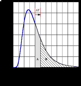
24 P(T,ΔT )= T+ ΔT T T f (t)dt f (t)dt (6.27) where f(t) is the probability density function for the earthquake recurrence intervals. Several difference forms of the distribution of earthquake recurrence intervals have been used: normal, log-normal, Weibull, and Gamma. In engineering practice, the most commonly used distribution is the log-normal distribution. The lognormal distribution is given by (eq. 4-19): f LN (t)= 1 2πσ ln t t (ln(t) ln(µ))2 exp 2 2σ ln t (6.28) Although lognormal distributions are usually parameterized by the median and standard deviation, in renewal models, the usual approach is to parameterize the distribution by the mean and the coefficient of variation (C.V.). For a log normal distribution, the relations between the mean and the median, and between the standard deviation and the C.V. are given in eq and 4.21: T µ = 2 exp(σ ln t /2) (6.29) σ ln t = ln(1+ CV 2 ) (6.30) The conditional probability computed using the renewal model with a lognormal distribution is shown graphically in Figure In this example, the mean recurrence interval is 200 years and the coefficient of variation (C.V.) is 0.5. The conditional probability is computed for an exposure time of 50 years assuming that it has been 200 years since the last earthquake. Graphically, the conditional probability is given by the 6-24

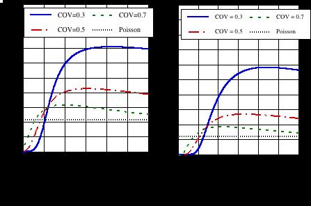
25 ratio of the area labeled A to the sum of the areas labeled A and B. That is, P(T=200,ΔT=50)=A/(A+B). An important parameter in the renewal model is the C.V.. The C.V. is a measure of the periodicity of the earthquake recurrence intervals. A small C.V. (e.g. C.V. < 0.3) indicates that the earthquakes are very periodic, whereas a large C.V. (e.g. C.V>>1) indicates that the earthquakes are not periodic. Early estimates of the C.V. found small C.V. of about 0.2 (e.g. Nishenko, 1982); however, more recent estimates of the C.V. are much larger, with C.V. values ranging from 0.3 to 0.7. In practice, the typical C.V. used in seismic hazard analysis between 0.4 and 0.6. The sensitivity of the conditional probability to the C.V. is shown in Figures 6-11 and 6-12 for a 50 and 5 year exposure periods, respectively. For comparison, the Poisson rate is also shown. These figures shows that the renewal model leads to higher probabilities once the elapse time since the last earthquake is greater than about one-half of the mean recurrence interval. In addition, these figures show that as the C.V. becomes larger, the conditional probability becomes closer to the Poisson probability. Figures 6-11 and 6-12 show one short-coming of the lognormal distribution when applied to the renewal model. As the time since the last earthquakes increases past about twice the mean recurrence interval, the computed probability begins to decrease, contrary to the basic concept of the renewal model that the probability goes up as the time since the last earthquake increases (e.g. strain continues to build on the fault). To address this short-coming of the lognormal model, Mathews (1999) developed a new pdf for earthquake recurrence times called the Brownian Passsage Time (BPT) model. The pdf for this model is given by: f τ BPT (τ,cv ) = 1 2 (τ 1) exp (6.31) 2πCV 2 3 τ 2CV 2 τ 6-25

26 where τ is the normalized time since the last event:τ = t T. The pdf for the lognormal and BPT model are compared in Figure 6-13 for a CV=0.5 and a mean recurrence interval of 200 years. These two pdfs are very similar. The difference is that the BPT model puts more mass in the pdf at large recurrence times that avoids the problem of the probability reducing for large recurrence times. This increase in mass at large recurrence times is shown in Figure 6-14 which is a blow-up of the pdf shown in Figure Another difference between the lognormal and BPT models is a very short recurrence times. At short recurrence times, the BPT model has less mass than the lognormal model as shown in Figure This will lead to lower earthquake probabilities shortly after a large earthquake occurs. The probabilities computed using the lognormal and BPT models are shown in Figure 6-16 for a mean recurrence of 200 years and a CV of 0.5. This figure shows that the BPT model is very similar to the lognormal model, but does not have the undesirable feature or descreasing probabilities for long recurrence times. For this reason, the BPT model is preferred over the log-normal model. 6-26

27 Figure 6-1. Relations between the different magnitude scales. (From Boore and Joyner, 1982). All of the magnitude measures, other than moment magnitude saturate at some maximum value due to low frequency limits of the magnitude measures.

28 Figure 6-2. The maximum magnitude is the magnitude at which the pdf goes to zero. \

29 Figure 6-3. Comparison of magnitude-area scaling for constant stress-drop with width limited L-models.

30 Figure 6-4. Comparison of the magnitude-area scaling for regression of M given log(a) and the regression of log(a) given M.

31 Figure 6-5. Comparison of magnitude pdfs commonly used in seismic hazard analyses

32 Figure 6-6. Comparison of the exponential recurrence model with paleoseismic estimates of the recurrence for large magnitude earthquakes (From Youngs and Coppersmith, 1985

33 Figure 6-7. Example of catalog completeness evaluation for the San Francisco Bay Area seismicity. (From Geomatrix, 1993). For short time intervals (left and side of plot) there is large natural variation in the seismicity rates. For long time intervals (right side of plot), the seismicity is expected to become constant. A significant decrease in the rate for small magnitudes as compared to large magnitudes indicates that the catalog is not complete for the smaller magnitudes. The years marked in the plot indicate the estimated completeness periods.

34 Figure 6-8. Comparison of exponential recurrence model using least-squares and maximum likelihood.

35 Figure 6-9. Comparison of recurrence relations for the commonly used magnitude pdfs.

36

37

38 Figure Comparison of the pdf for the lognormal and the BPT model. In this example, the mean recurrence interval is 200 years and the CV =0.5.

39 Figure Comparison of the pdf for the lognormal and the BPT model. In this example, the mean recurrence interval is 200 years and the CV =0.5. The figure has expanded the tails of the distribution to show that the BPT model has more mass than the lognormal model.

40 Figure Comparison of the pdf for the lognormal and the BPT model. In this example, the mean recurrence interval is 200 years and the CV =0.5. The figure has expanded the small recurrence tails of the distribution to show that the BPT model has less mass than the lognormal model for short recurrence times.

41 Figure Comparison of the probability of an earthquake for the lognormal and the BPT model. In this example, the mean recurrence interval is 200 years and the CV =0.5.