Dispersion Technology DT1200. Operating and Maintenance Manual

Transcription

1 Dispersion Technology DT1200 Operating and Maintenance Manual Dispersion Technology 364 Adams Street Bedford Hills, NY Wednesday, May 30, 2007 Software Version

2 Table of Contents 1. Basic Operating Instructions... 6 Introduction... 6 Measurement Overview... 6 Getting started - Turning on power and starting software... 6 Log in Log-out or Log-in again Adding a new user Editing an existing user Getting familiar with the basic sensor configuration Emptying and cleaning the chamber, basic sensor configuration Filling the empty chamber with a new sample, basic configuration Stirring the sample, if equipped with dc motor Stirring the sample, if equipped with digital stirrer Initializing the burettes Setting up burettes with 1 Normal Acid and Base Reagents Using the Holder for storing ph probe when not in use Placing ph probe in sample Measuring ph and temperature Checking system by measuring intrinsic attenuation of water The Status Bar Viewing the attenuation of the water sample Preparing a 10 wt% colloidal silica sample Defining the 10 wt% colloidal silica sample Using the Content Wizard Using pyncnometer tool to determine weight fraction of sample Measuring attenuation and calculating psd, 10 wt% silica Getting familiar with the Analysis form Printing and Saving Analysis as a Test Report Saving any graph on the Analysis as separate picture Saving and retrieving Excel files from the Analysis form Re-calculate option - Selecting a particular record Re-calculate option - Prediction Re-calculate option - Overlay several records Re-calculate option - Volume fraction search Re-calculate option - Scattering coefficient search Re-calculate option - Thermal expansion coefficient search Re-calculate option - Structure and Fractals Re-calculate option - Mixtures of two dispersed phases Saving intrinsic attenuation Understanding Experiments and Measurements Time Titration Protocol, zp of 10 wt% colloidal silica Viewing Continuous data Getting familiar with Burette Control in manual mode Titration protocol ph ramp, measuring zp of 10 wt% colloidal silica

3 Using Details in ph ramp Titration Protocol (optional) ph Stat titration protocol ml titration protocol, 10 wt% colloidal silica Simple colloid titration without measurements Continuous temperature control of sample Ramp Temperature Protocol using 10 wt% Silica Ludox sample Making plots of existing data Saving graphs to metafiles Adding a saved graph to a document Viewing Data Opening the Data View window Finding specific data Reading and revising comments in the data Getting a quick overview of a large set of data Selecting data fields to be displayed Creating a custom view of the data Editing your measured data using the Data View window Re-analyzing selected experiments Exporting selected experiments to Export directory Reviewing exported files Sending an export file by Saving all Experiments in a Query to an Excel Spreadsheet Reviewing Properties of Materials Displaying Basic properties of a solid material Displaying Basic Properties of a Liquid material Displaying material properties at a specific temperature Sorting materials by a given material property Displaying Standard, User defined, and Favorite materials Saving Material Properties to an Excel Spreadsheet Displaying Details of a Material Comparing the properties of two materials Defining a new solid material General comments Defining a new solid material for making submicron particles Defining density of new solid material using pyncnometer and slurry Using pyncnometer bottle to determine density of particles in slurry Sensitivity of particle density measurement to slurry weight fraction Deleting a material Defining a new solid material for making large particles Defining a new solid material for making soft particles Defining Thermal Expansion Defining Thermal conductivity Defining Heat capacity Defining a new material based on an existing material Defining a new liquid material General comments Defining new liquid material - as medium for solid particles Defining Density

4 Defining Viscosity Defining Dielectric constant Defining Sound speed Defining Intrinsic loss Automatic determination of Sound speed and Intrinsic loss Saving the newly defined material Defining a new fluid material as medium for soft particles Thermal conductivity Heat Capacity Thermal Expansion Defining new liquid material - for emulsion droplets Define New Material form Set up instrument to work with an external pump Loading sample using external pump Emptying the sample using external pump Using zp probe externally Using zp probe externally with ring stand Advanced Topics Viewing more Raw Data Grid information Calculating the density of material using pyncnometer Calculating weight fraction of sample using pyncnometer Using Setup parameters Using single gap mode to study structure Measuring zp at high ionic strength Measuring Complex samples Computing zeta potential for bimodal size distributions Measuring weight fraction from cvi Calibration Temperature calibration ph calibration Conductivity calibration Zeta potential calibration Pyncnometer calibration Viewing Calibration Constants Error in one or more Calibration constants Definition of instrument Constants Acoustic Sensor Conductivity NonAq Conductivity probe ElectroAcoustic Impedance probe Interface ph probe Pyncnometer Sample Signal Processor

5 Temperature probe Wfr calibration Maintenance Replacement of consumable items Acoustic chamber, checking seals Burette, rinsing Electroacoustic probe, cleaning Measuring Unit, cleaning ph probe, preparing for use ph probe, cleaning ph probe, filling ph probe, restoring response Sample chamber, cleaning Sample Handling systems of the DTI instruments DT-300, Electroacoustic Zeta Potential Probe Zeta Probe, manually Zeta Probe supported with the holder plate Zeta Probe up side down with small sample cup Zeta Probe with magnetic stirrer Zeta Probe with peristaltic pump DT-100, Acoustic particle size sensor DT-100 with minimum sample volume DT-100 with peristaltic pump DT-100 with magnetic stirrer DT-100 with titration setup DT-1200, Acoustic and Electroacoustic spectrometer DT-1200 with magnetic stirrer DT-1200 with peristaltic pump DT-1200, separate sensors DT-400, Titrator DT-500, On-line sensor block DTI additional sensors Conductivity Dielectric permittivity Appendix A Setting up instrument for a specific customer Appendix B Retrieving Data from Database with a Query

6 1. Basic Operating Instructions Introduction It is suggested that any new user of the DT1200 use the following tutorials as a means of becoming familiar with the instrument, before attempting to make measurements on their own. Each lesson builds on the skills learned in the previous one so it is best if you go through the lessons in the order presented. In some cases individual lessons can be skipped if you are in hurry to get started, and these lessons are marked optional. This manual describes all of the features and capabilities of a complete DT1200, with all available options. Your instrument may not have some of this optional equipment and you can simply ignore those sections that do not apply to your case. Measurement Overview Making a measurement and printing the results is simple. This lesson provides a quick overview of the sequence of steps necessary to do a single measurement. Succeeding lessons describe these steps in more detail to answer any questions. This lesson assumes you are using the instrument in its basic configuration, i.e. all sensors combined into a single assembly mounted in the Measuring Unit. There are 10 steps to making a single measurement, 1. Empty any sample from the chamber. 2. Fill the chamber with your new sample. 3. On the Home page, click on each type measurement that you want to perform. 4. Select the name of the media from list of materials. 5. Select whether your disperse phase is a solid or liquid. 6. Select the name of the disperse phase from list of materials. 7. Enter the weight fraction of your sample. 8. Press the Run button. 9. Wait till the measurement is complete, and the analysis of results appears. 10. On Analysis report, click on File- Print report. Getting started - Turning on power and starting software For convenience, you can leave the system always turned on, with the DT1200 software running, so that it will always be available for measurements as needed. Turning on the DT1200 is a two step process. First turn on the Electronics box by depressing the power button on the front panel. Next, turn on the computer. It is important that the Electronics Unit be turned on first so that the Plug and Play feature of Windows can install the correct software for the plug-in cards in the Electronics Unit. The Windows operating system should be open within a minute or so. 6

7 If the DT1200 is already powered up, check to see if the DT1200 program is running. If it is running, either the Home window will be visible, or it will be minimized and shown only as an icon on the bottom status bar. If program is running but minimized, click on DT1200 icon on the status bar at the bottom of the screen. If the DT1200 program is not Figure 1-1 Display screen showing Home page running, double click on the DT1200 icon which appears on the desktop, as shown at left side of screen in the figure to the right. Each time the DT1200 program starts it performs tests to check the performance of each installed component. The Instrument Status form, showed below, indicates the status of each component as the test proceeds. 7

8 Figure 1-2 Instrument Status form When the tests are complete a message box, such as shown below, will appear that asks if you want to initialize the burette now. Answer No, as we will do this later. 8

9 When the start-up tests are complete, the Home page will appear as shown below in Figure 1-3. Figure 1-3 Home page at start-up 9

10 Log in Before making measurements it is useful to log in. If you are logged in any measurements that you make are automatically saved with reference to your initials and project name. This will make it easy for you to later find specific test results. After the system has completed its startup sequence, you can log in by clicking on LogIn/Out on the home page menu bar. The LogIn form shown to the right form will appear. The password for a Guest user is simply the word guest. Type guest in the password box and press the Enter key. Case is not important. The window will then appear as shown below. If you wish you can then enter a description of the project you are working on in the Project box. This information can be used later to retrieve specific data related to your project. For now, if you like, just type the phrase my first measurements. Every person logged-in is defined in the saved data by his/her Initials. As shown in the Initials box, the initials for a Guest is Gst. (The initials for an existing User Name can not be changed.) To log in press the Log In button. 10

11 Log-out or Log-in again If you are through using the instrument you may want to log out so that another user does not inadvertently make measurements and save data marked with your initials and project. To log out click the menu item LogIn/Out on the Home page. A window such as the one shown to the right will appear. To log out press the Log Out button. If you wish, you can enter a different Project and then press Log In. If you decide not to logout press Cancel. 11

12 Adding a new user Click on LogIn/Out on the home page to display the Log In Window. From the list of User Names select Administrator. Enter the Administrator password and press the Enter key. (The Administrator password is dispersion.) To add a new user or edit an existing unit press the Add/Edit Users button. The Add/Edit User window will appear. Enter the new User Name, e.g John Smith, and press the Enter key. 12

13 A window Defining new user John Smith will appear. Enter a password for the new user and then press Enter key. The password will be visible during entry. If you like, enter a more appropriate three letter initials for this new user. (By default program picks first three letters of first name. Use care picking initials; once initials are saved for this user, the selected initials can not be changed.) If you wish, you can also define address of this user. (This will be of use in communicating in the event that you have questions concerning the results or have service related questions.) By default, a new user is defined to have User, Guest, and Reader privileges. If appropriate for this individual, you can add Expert and/or service privileges by checking the appropriate boxes. To save this new user definition, press the Save button. To forget this new user definition, press the Cancel button. 13

14 Editing an existing user The procedure for editing an existing user is very similar to defining a new user. Click on LogIn/Out on the home page to display the Log In Window. From the list of User Names select Administrator. Enter the Administrator password and press the Enter key. Press the Add/Edit Users button. The Add/Edit window will appear. Click on the box to the right of the User Name box to pull down list of existing users. Select an existing user, e.g. John Smith. The password for this user is visible. You may change the password if you wish. You may also change the address for this user. You can also change the privileges for this user by checking or un-checking the privileges boxes at the bottom of the window. To save your changes for this user, press the Save button. To forget changes for this user, press the Cancel button. 14

15 Getting familiar with the basic sensor configuration In the basic sensor configuration the acoustic, cvi, temperature, and conductivity sensors are all installed together so as to form a common sample chamber. The chamber is mounted inside the Measurement Unit, which is depicted in Figure 1-4. A top and front cover protects the sensors from exposure to spilled sample or cleaning fluids. Some users prefer to work with the covers removed. The top cover can easily be removed by first removing the knurled ring around the entrance port and lifting the top cover. Figure 1-4 Measuring Unit with covers removed Emptying and cleaning the chamber, basic sensor configuration The chamber should always be left filled with some appropriate clean storage fluid, e.g. water. This will keep any residual contaminants from drying out on the surfaces, in which case they would be more difficult to remove. Your first step in measuring a new sample is to empty any storage fluid or any previous sample. 15

16 If the ph probe is inserted in the cap, remove it and insert it in the storage fixture for now. Remove the cap at the top of the chamber and put it aside. Place a beaker below the chamber and open the rotary or pinch valve to allow the sample to run out. Close the valve or pinch clamp. Fill the chamber with some appropriate cleaning fluid depending on the last sample that was measured (e.g. plain water, water with detergent, solvent, etc). For now, we will use just plain tap water. If necessary, use the supplied nylon brush to clean the chamber. Note: It is not important that the chamber be spotlessly clean. Some discoloring of the walls of the chamber after using various pigments is not a problem. This is one of the advantages of working with concentrates; they are not easily contaminated in a significant way. Open the valve again, let the sample run out, and then close the valve again. Continue on to next lesson. Do not stop here! We always want to leave the chamber filled with fluid when not being used. If the chamber is left empty, any residual contamination will dry on surface and may later be difficult to remove. Wet surfaces stay cleaner than dry surfaces. Filling the empty chamber with a new sample, basic configuration Empty the chamber of any fluid as described above. Close the valve on the exit port of the chamber. Turn off the stirrer. The basic configuration requires about 120 ml of sample. Fill the chamber with sample as shown in figure to the right. As the sample chamber is filled, the fluid will also rise in the external bypass tube that connects the bottom to the top portion of the sample chamber. The sample chamber should be filled till the fluid reaches the return port at the top of the chamber. It should not be overfilled since, as the acoustic sensor closes, the level will rise approximately 6 mm further. 16

17 Figure 1-5 Filling the chamber 17

18 Stirring the sample, if equipped with dc motor Turn on the stirrer. The stir bar acts not only as a normal vortex stirrer but also as a centrifugal pump, causing the sample to be circulated from the bottom, up the external tube and back to the top via the return port. The speed of the stir bar is controlled by a rotary switch on the bottom of the stirrer assembly as shown in figure to the right. Start by turning the stir bar off by turning the control fully counter clockwise (viewed from below). Increase the setting one step at a time, waiting a few seconds at each position. Find the fastest setting at which the sample is stirred well. If the speed is too fast, the stir bar will decouple, and the sound will change significantly. It is best to work at that speed setting just one step slower than the highest one that appears to work reliably. Sometimes a bubble is trapped in the chamber. It is useful to turn the stir bar off for a few seconds, and then turn it back on. This usually dislodges any large air bubble and brings it to the surface. Figure 1-6 Set stir speed Stirring the sample, if equipped with digital stirrer If your unit is equipped with a digital stirrer the speed is controlled from the keyboard. The digital stirrer provides constant speed, independent of the viscosity of the sample. The stirrer can be turned on by clicking on the stir button at which point it will turn red to indicate the stirrer is on. If you click the button again the stirrer will turn off and the red light will go out. You can adjust the speed by first displaying the desired speed (using the list box scroll keys) and then clicking on it so that it is displayed with blue background. The indicated value is the stir speed in revolutions per second. It is sometimes more convenient to change speed using the UP/Down keys on the keyboard which works immediately after you turn the stir motor on. Sometimes it is convenient to have the stirrer turn on automatically whenever you start a new experiment. You can arrange this on the Home Page by clicking on Tools Options 18

19 and then checking the box AutoStir On at Start of Experiment as shown in figure below. In a similar way you can arrange to turn off the stirrer automatically at the end of an experiment by checking the box AutoStir Off at End of Experiment 19

20 Initializing the burettes Each burette must be initialized before it can be used to dispense reagent. After the burette is initialized, it then knows the position of the syringe plunger and how much reagent is left in it that can be dispensed. If you are not planning to use the burette to dispense reagents you can skip this step. You can always initialize the burette later, but you will have to empty any sample before doing so, or some unspecified amount of both reagents will be added to the sample. Some of the following lessons do use the burettes, so let s initialize it now. The two burettes are shown in the Figure to the right. On the Home page, click on the menu item View - Burette control. The Burette Control form appears as shown in Figure 1-7 figure below. By default, it is assumed that 1 N HCl is installed in Burette 1 on the right and 1 N KOH is installed in Burette 2 on the left, but this can be changed as will be shown later. Click on the Initialize button for Burette 1. The plunger moves to empty the contents of the syringe into the sample, and then only partially fills it with fresh reagent. Notice that after initialization the Initialize text changes color to green. Next initialize the second burette in the same way. Figure

21 Setting up burettes with 1 Normal Acid and Base Reagents If your burettes are already set up with 1N acid and 1 N base reagent, then you can skip this lesson if you are in a hurry. However, if you plan to use other reagents in your work and you want to understand how to load the burette with fresh reagents, proceed as follows. Click on the first pull down box at the top of the form for Burette 1. The message shown below appears. Click Yes to continue. Click on Acid. In the lower pull-down box below, select 1 N HCl. The message shown below will appear. Follow the instructions and then click OK. The message shown below then appears. Follow these instructions and then click OK. Finally, the following message appears. Click OK. Then Click the Flush button for burette 1. Notice that the syringe first pulls in a small amount of air, then some fresh reagent from the bottle. Then it dispenses this volume of air and reagent to the sample via the dispensing probe. This sequence of partially filling the 21

22 syringe with air and reagent is repeated three times. The purpose of this operation is to remove any trace of the previous reagent. At the end of the flush cycle the burette is empty of any air and contains only some new reagent. Click the fill button for burette 1. Note that the syringe moves all the way down, filling the syringe with 5 ml of reagent. You can also empty the syringe by clicking of the Empty button, but we will not do that just now. Instead we will manually dispense a specified dose of reagent. Click on the pull down box for the dispense volume for Burette 1. Select a dose of 100 ul. Click on the Dispense button to dispense this volume of reagent. Note that even this small dose is not dispensed suddenly, but instead dispensed slowly over the next 10 seconds or so. This is done so as not to shock the system by adding reagent too quickly. Repeat the same process for Burette 2 using 1 N KOH. Then Empty the Chamber and refill with distilled water. Using the Holder for storing ph probe when not in use If the ph probe is still packed, prepare it using the Maintenance Procedure ph probe, preparing for use before continuing. When the ph probe is not being used, it should be stored safely in the storage fixture shown below. The storage fixture should be filled with ph probe filling solution. The nut should be tightened sufficiently that the ph probe fits snugly into the receptacle, but not so tight that it is difficult to remove. The tip of the ph probe is very delicate and easily broken. Use caution moving ph probe from place to place. Placing ph probe in sample Install the cap on top of the Chamber. It is held in place with an O ring around the side. Twist it slightly while pushing downward so that it is seated on the top flange of the chamber. Make sure that the ph probe has been properly prepared for measurements. It is important that the ph probe is not inserted too far, or the probe will be broken during attenuation measurements as the gap is closed! The tip of the probe should extend at least 40 mm from the bottom of the cap, but no more that 45 mm. Carefully insert the ph probe into the Cap as shown in figure to right. Figure 1-9 ph probe in sample 22

23 Measuring ph and temperature A platinum resistance temperature probe is installed in the bottom sensor block and protrudes about 10 mm into the sample so as to precisely monitor the sample temperature. The present value of the sample temperature is displayed on the Home page. Check that the temperature displayed is reasonable. There may be times when you want to enter the sample temperature manually, instead of measuring it. Double click on the label Temp, C on the Home page. Note that this label becomes red in color, indicating that it is no longer being measured. Now type in any temperature value, e.g This new value will be accepted and, in fact, will be recorded in the database as if it were the actual temperature at which succeeding measurements are made. Double-click again on the temperature label, and note that the label returns to the original color and that the temperature displayed is again the actual measured value. It is important to understand that the temperature that is entered does not control the temperature; it only sets the temperature that will be recorded to the database for succeeding measurements. The ph of distilled water, after it has come to equilibrium with CO2 in the atmosphere is about 5.5. Check to see that the ph is reading in the range of 5-6. The ph value can also be entered manually in the same way as temperature. Double-click on the label ph. The label text turns to a red color. You can now edit the ph value. This value will be recorded in the database for all succeeding measurements until the box is double-clicked again. Double-click again on the ph value to return to monitoring ph. Figure 1-10 Manual entry of ph and temperature data 23

24 Checking system by measuring intrinsic attenuation of water The DT1200 measures attenuation over a very wide dynamic range. Pure water has an attenuation which is less than any of the colloids that you might be interested in, so it is a convenient sample for testing the performance of the instrument at an extreme condition. In the Experiment design frame, click the Attenuation button so that it is checked. If necessary, click on other buttons so that none are checked. In the Sample definition frame, see that the Liquid media is water and the particles are defined as none. This is the default condition when the program starts, so you will not need to make any changes if you have been following these lessons in order. Press the Run button. The following message will appear since we have not yet defined any disperse phase. We do in fact want to measure the intrinsic attenuation of water, so click Yes. The Run button will initially change to Starting and then split into two separate buttons labeled Stop and Pause. We will discuss the functions of these buttons later when doing more complex titration experiments. The Status Bar The status bar at the bottom of the home page, shown in Figure 1-11, is divided into two parts. The left hand portion of the Status Bar gives information as to what the system is doing right now. During the attenuation measurement running now it will tell you that it is measuring attenuation and will specify which gap is presently being used to collect data. The right hand portion of the Status Bar indicates the amount of time required to complete the current experiment. In this case the experiment is quite simple, a single attenuation measurement. For a single measurement this information is not so helpful, but when doing a long titration experiment it will tell you how much longer it will take to complete the experiment. 24

25 Figure 1-11 Status bar on Home page 25

26 Viewing the attenuation of the water sample When the measurement of your water sample is complete, the Status Bar at the bottom of the home page will indicate the time that this simple experiment was completed. On the Home page, click on View Grid Raw Data. The Grid form will open. Click on the menu item View Attenuation and the attenuation for the water sample you just measured will appear, similar to that shown in Figure Figure 1-12 Attenuation of water The attenuation of water at 100 MHz varies from to db/cm/mhz depending on the room temperature. Two curves are shown in the figure. The top curve, described by the solid circles, shows the measured attenuation. The bottom curve, described by the x symbols, shows the expected error for each measured attenuation. Typically the error increases as the frequency decreases, as shown in this example. The error will usually be less than 0.05 db/cm/mhz at 3 MHz. 26

27 Preparing a 10 wt% colloidal silica sample The next several lessons use a 10 weight % dispersion of colloidal silica. It is supplied in liquid form at a concentration of 50 wt% and must be diluted prior to measurement with 0.01 M KCl. The following procedure will prepare a sample of about 120 ml which is sufficient for making measurements using the basic sensor configuration. Prepare a liter of 0.01 M KCl by adding.745 g of Potassium Chloride to a 1 liter volumetric flask and filling flask to 1 liter using distilled water. Place a 250 beaker on a balance and tare it. Weigh out 25 g of the 50% concentrate. Dilute this to a total weight 125 g using 0.01 M KCl as diluent. This sample will be used both as a demonstration colloid for illustrating particle size and as a zeta potential standard. The particle size measurement does not require any calibration. Once a sample has been prepared by dilution, it should be used that day and then discarded. Although the 50% concentrate is stable for a long time, the ph and zeta potential value of the diluted sample will change slowly with time. Defining the 10 wt% colloidal silica sample If we only want to measure the attenuation and sound speed of the sample, we do not need to know anything about the properties of the sample. However, if we want to calculate the particle size distribution we need to know some physical properties. For sub-micron rigid particles such as silica we need to know only the density of both the particles and the media, and also the viscosity of the media. Since we want next to measure the PSD of this colloidal silica, we need to define this sample. This is done in the Sample Definition frame on the Home form shown in Figure First we define the liquid media. Water is selected by default when the program starts and we will use this default value for our silica sample. The required density and viscosity for the selected media is automatically computed from information in the Material Table in the database. 27

28 Figure 1-13 Defining the 10 wt% colloidal silica Next we need to define the particles, i.e. the disperse phase. By default, the particles are assumed to be solid. Since our silica particles are indeed solid, we keep the default condition. Next we need to specify the material that our particles are made of, in this case silica. To do this we use the pull-down box to display a list of pre-defined materials that are saved in the Material Table in the database. If we type the letter s the list will display those materials starting with the letter s. Accordingly we select the material silica, Ludox. The required density of the particles is calculated from data in the Material table. Once we have defined the materials that compose our colloid, we need to then specify how much of each material is present in our sample. This is done inside the Content frame. In this simple case we can simply type the weight % inside the appropriate box in the content frame as shown in Figure

29 Using the Content Wizard Sometimes you may not know the weight fraction of the sample you want to measure but you do know other information about the weight or volume of the media, disperse phase, or the sample as a whole. The DT1200 provides a Content Wizard that can help you define the weight fraction of the sample given various combinations of known information. To demonstrate, click on the menu item Tools Content Wizard. The content portion of the Home page expands to add boxes for %vol, weight(gm), and volume (ml) for the media, disperse phase and for the sample as a whole, as illustrated in Figure Figure 1-14 Using the Content Wizard Let us say that we have prepared 125 g of our 10 wt% silica Ludox standard material. Enter this value for the total weight of the Disperse system. Then click on the Calculate button. The values for the weight, volume and vol% are then computed for the disperse phase, the media, and the overall system, as shown in Figure For example, we see that the 10 wt% silica sample consisted of 12.5 g in a total sample volume of ml. The values you entered are shown in red; the computed values are shown in blue Figure 1-15 Entering wt% and the total weight to calculate all other parameters 29

30 The content wizard can be used to calculate the weight fraction of a sample given any sufficient combination of weight, or volume information. For example, in the current case we saw that the 10 wt% silica sample consisted of 12.5 g in a total sample volume of ml. We could just as easily have entered this information to define the sampleand then press the Calculate button as shown in Figure Figure 1-16 Entering weight of particles and total volume to obtain all other parameters 30

31 Using pyncnometer tool to determine weight fraction of sample Sometimes you may be given a sample where the weight fraction is unspecified. Perhaps someone else prepared the sample and didn t tell you the weight fraction of the particulates. Let s say that you know only that your sample is alumina_alpha dispersed in water. Your Sample definition would appear as follows, with the wt% left blank. To determine the wt%, click on Tools Pyncnometer on the Home page. The following window will appear. The Sample definition on the Pyncnometer form will automatically be preset to the sample that you have already defined, i.e. alumina_alpha in water.. If you are using a density meter, just enter the measured temperature and the density of the slurry and press Enter. For example let s say you measure a slurry density of at 31

32 at a temperature of 23.6 C. The pyncnometer form would appear as shown below with a Weight % of shown in the Calculated results.. If you press the Save button, the weight % value will automatically be saved to the wt % box on the sample Definition frame on the Home page. If you do not have access to a very handy density meter, you may want to use a simple pyncnometer bottle to determine the weight % of your sample. A pyncnometer bottle is simply a bottle that allows one to fill it with a very well-defined volume of fluid so that this precise fluid volume can be weighed accurately. If you check the menu item Options Use pyncnometer bottle, the pyncnometer window will appear with two extra boxes, one containing the calibration constant for the pyncnometer volume, and a second labeled Weight,g for entering the measured weight of the fluid contained in the pyncnometer bottle. \ 32

33 If the value for the pyncnometer volume is blank then it is clear that your pyncnometer bottle is not calibrated. To calibrate the pyncnometer bottle, click on Calibration Pyncnometer on the Home page and follow those instructions. Once the pyncnometer is calibrated, the unknown weight fraction of your sample can be determined as follows: 1) Clean and thoroughly dry the pyncnometer bottle and the stopper. 2) Place the empty dry pyncnometer bottle and stopper on balance and tare it. 3) Measure the temperature of your slurry sample. 4) Remove the pyncnometer bottle from the balance, fill the pyncnometer bottle with your sample, carefully insert stopper so that excess fluid fills and overflows the capillary in stopper, and carefully remove any excess fluid from the outside of the bottle. 5) Place filled pyncnometer bottle on balance and weigh contents of the bottle. 6) Enter the temperature and measured weight on the Pyncnometer form. 7) Press Compute to calculate and display the weight fraction in the Calculated results frame. 8) Press Save to enter the measured weight fraction for your sample as the wt% in your Sample definition on the Home page. For example, let s say that you have filled the pyncnometer with your slurry and have determined that this volume of slurry at 23.6 C weighed grams. If you enter the temperature and measured weight in the respective boxes on the Pyncnometer form, it would then appear as shown below. The calculated weight % is the same as we measured previously using the density meter. If you now click on the Save button, the calculated weight % will be automatically input to the wt% box in the Sample definition frame on the Home page as shown below. 33

34 34

35 Measuring cvi and calculating zp, 10 wt% silica sample Let s determine the zeta potential of this 10 wt% colloidal silica. We have already defined the sample. The next step is to define the experiment that we want to do by checking the appropriate boxes in the Experiment Design frame. We want to measure zp, so we need to check the box labeled CVI for zeta potential as shown in Figure When we do this the A priori frame appears asking us to define the particle size of the sample. The calculation of zeta potential requires size information if the size is larger than about 0.3 microns. Below 0.3 microns, the calculation of zeta potential is independent of particle size. The colloidal silica has a size of about 0.03 microns, so we can just leave the value set to the default value of 0.1 micron. Figure 1-17 To make the measurement, click on Run. If we are asking to measure only zeta potential, but not particle size, the following message will appear asking for some particle size information. If the particle size is less than 300 nm then the size information is not necessary to compute the zeta potential and you should check the first option, Particle size is less than 300 nm. If the particle size is larger than 300 nm and is known, then enter the estimated size and the standard deviation in the respective boxes, and then check the second option box Particle size is known. If the size is unknown, then check the third option box, Particle size is unknown. 35

36 After a few seconds, the Home page will appear as shown in Figure The left portion of the Status Bar indicates that the unit is now measuring the colloid vibration current. Figure 1-18 After a short time, the measurement is complete and the Analysis form appears with the calculated zeta potential, as shown in Figure The value should be approximately - 38 mv. The calibration of zeta potential is discussed in the Calibration chapter. Figure

37 Measuring attenuation and calculating psd, 10 wt% silica. We have already defined the sample for our 10 wt% silica. Click on the Attenuation box till it is checked. For now, make sure the Conductivity and CVI boxes are not checked. Click on either if necessary to uncheck it. Click the Run button. It will take several minutes to measure the attenuation spectrum. During this time you will get updates in the left-hand side of the Status Bar as to which gap is being measured. Eventually the Analysis form, similar to that shown in Figure 1-20, will be displayed showing the particle size distribution for this sample. Figure 1-20 Analysis of PSD for colloidal silica 37

38 Getting familiar with the Analysis form In this lesson we will learn more about some detailed capabilities of the Analysis form. This form appears right after the raw data has been collected. The main purpose of the Analysis form is to convert the raw data, such as attenuation or colloid vibration current, to the user required outputs, such as particle size and zeta potential. It performs these calculations and then displays the output results. If the Analysis form is not currently displayed, click on the menu item File Analysis on the Home page. The form s appearance depends on which raw data are measured for a particular record. There are four main display setups, namely: Setup 1) Acoustic attenuation and colloid vibration current are both measured. Setup 2) Only acoustic attenuation is measured; Setup 3) Only colloid vibration current is measured; Setup 4) Only acoustic attenuation is measured, but no disperse phase is specified on the Home form The following Figures illustrate these four display Setups, as they would normally appear automatically after a measurement is finished and the analysis of the raw data is complete. Each setup display Setup is largely fixed by the properties that are measured, but some modifications are possible by making selections from the View menu as will be described. Figure 1-21 shows Setup 1 for which attenuation, cvi, and conductivity are all measured. Whether the unimodal or bimodal PSD is shown depends on which provides the most realistic picture of the sample based on the respective fitting errors. Figure 1-22 shows Setup 2 for which only attenuation measured. In this case the fitting errors suggested that the bimodal solution provided a better representation. Figure 1-23 shows Setup 2 again, but in this case the user has clicked on the menu item View both unimodal and bimodal to see both. Figure 1-24 shows Setup 2 yet again, but in this case the user as clicked on the menu item View Sound speed to display sound speed information. 38

39 Figure 1-21 Setup 1 - All parameters measured, showing unimodal PSD Figure 1-22 Setup 2 - Only attenuation measured, showing bimodal PSD 39

40 Figure 1-23 Setup 2 - Only attenuation measured, showing unimodal & bimodal Figure 1-24 Setup 2 - Only attenuation measured, showing sound speed 40

41 The Analysis software can utilize altogether three separate theories of increasing sophistication for calculating zeta potential, namely the simple classic theory of Smoluchwski, an Advanced CVI aqueous theory, and a theory for non-aqueous or nanocolloids. Figure 1-25 shows Setup 3, for which we measure only CVI, and by default calculate zp using this classic theory. The more sophisticated theories yield more accurate zp values only when the conductivity of the sample is known, which in turn allows us to calculate the Debye length and Dukhin number Du, both important characteristic of surface conductivity. The Advanced CVI aqueous theory works when ka >3. For lower ka values, due to the small size or low ionic strength, the third theory becomes employed. It takes into account the overlap of thick double layers. The best output for the third theory is surface charge. This parameter can be calculated without conductivity, assuming nevertheless a ka < 3. The calculation of a zeta potential would require conductivity data, which might be hard to obtain in non-polar liquids. In addition, this calculation is very non-linear. The software restricts the highest value of zeta potential for this third theory at 200 mv. You can see the results for the two more sophisticated theories by clicking on the menu item View Advanced CVI. Figure 1-26 shows Setup 3 for case where user has indeed measured conductivity and selected Advanced CVI. Figure 1-25 Setup 3 - Only zeta potential is measured Figure 1-26 Analysis software utilizes three theories for calculating zeta potential. 41

42 The Advanced CVI aqueous frame has a check box labeled zeta bimodal. If you check this box a Bimodal frame appears as shown in Figure 1-27 below. This would allow you to recalculate zeta for given CVI using a bimodal PSD that you specify in this Bimodal frame Figure 1-27 Bimodal frame is supplied to define PSD for calculating zeta potential Figure 1-28 shows Setup 4 for case where only attenuation is measured and there is no disperse phase. This Setup is used for intrinsic attenuation measurement. Once attenuation data is displayed in Setup 4 it can be converted to a reological format by checking the box rheology output and then pressing RUN ( If necessary click on Recalculate to make RUN visible) This will convert attenuation and sound speed into visco-elastic moduli as shown in Figure

43 Figure 1-28 Attenuation spectra Figure 1-29 Rheological spectra 43

44 Printing and Saving Analysis as a Test Report Click on File - Print analysis as report to print a copy of the present report to the printer Check File- AutoPrint if you want to generate this report automatically each time you make a measurement. If you modify the report format you can save this so that it will be used next time the system is started by clicking File-Save report setup. You can Paste this form as a report into the MS Word file. In order to do this, use Alt- PrintScr keys. This would copy the form to the clipboard. The form must have focus at this point, which is indicated by top bar being blue. Then open MS Word file and do Paste command. Analysis appears there as a picture. 44

45 Saving any graph on the Analysis as separate picture You can save any graph on the Analysis form as a stand alone picture. In order to do this, click right mouse button. The following form appears. Select tab System. The form would become like following. Frame Export Image allows you to save this particular graph as metafile. Use button Browse to select directory and then type name of the file. 45

46 Saving and retrieving Excel files from the Analysis form The analysis of a particular measurement can be easily saved to an Excel file. Corresponding functions are available from the Analysis, File. You can save file with your own name using following form. If saved automatically, the name of the file would be constructed from the measurement data and time. To see all the saved Excel files, click on File-Explore saved files. The windows Explorer will open (in directory c:\data_aco\excel) and you will see a listing of all saved files, including the one you just created, Myfile, as shown on the following Figure. Files with last letter A contain numbers for attenuation graph. Files with last letter P contain numbers for size graph. 46

47 ft(i) At(i) atlog(i) atbi(i) The columns are defined as follows Ft(i) Frequency, MHz At(i) Attenuation, db/cm/mhz Atlog(i) Attenuation of best fit unimodal distribution, db/cm/mhz Atbi(i) Attenuation of best fit bimodal distribution 47

48 The column in the spreadsheet can easily be graphed using excel by clicking on the appropriate columns and then clicking on the graph tool. A resulting spreadsheet with the graph might appear as shown. ft(i) At(i) atlog(i) atbi(i)

49 In a similar manner, we can look at the PSD data. In Windows Explorer, Click on the file myfilep.csv. A spreadsheet similar to this should appear. d-log psd-log cum-log d-bi psd-bi cum-bi psd-1 psd E E E E E E The columns are defined as follows. d-log Diameter for unimodal distribution data, microns psd-log Unimodal particle size distribution function cum-log Unimodal cumulative particle size d-bi Diameter for bimodal distributions, microns psd-bi Bimodal particle size distribution cum-bi Cumulative bimodal particle size psd-1 Particle size distribution of mode 1 of bimodal distribution psd-2 Particle size distribution of mode 2 of bimodal distribution Rheological data is saved automatically to the file "c:\data_aco\srhe.dat" If you want to save attenuation and PSD excel files for every measurement, the check File - Autosave If you want to see the last attenuation data that was analyzed, click on File- Open last attenuation with Excel. If you want to see the last PSD information that was generated by the Analysis form, click on File - Open last PSD with Excel. If you want to explore all Excel files created by the Analysis form, click on File - Explore saved Excel files. 49

50 Re-calculate option - Selecting a particular record. Analysis form can re-analyze existing raw data. To access previous data first click on the menu item Re-calculate. The Analysis form widens to show additional information as illustrated on the right-hand side Several objects in the frame database record select allow you to connect Analysis to any record from the database. As a first step you should select a Query that contains this record. This is done with the object that is linked to the query ~DemoQuery now. Clicking on arrow would open a list of available queries. As a second step you should select a database field for chousing the record. It is done with the list under the Query name. When you select the field it would show automatically all records of this query by the field values on the list below. Click on the record you want and Analysis would be automatically connected to it. Object with four arrows on the top of the frame allows you to browse records of the selected query. 50

51 Re-calculate option - Prediction. Button RUN starts calculation for the selected record. You can restrict frequency range for cutting off attenuation points that are in doubt. Use boxes fmin and fmax for this purpose. You can restrict size range using boxes dmin and dmax. You can recalculate automatically all records in the given query by checking box recordset Option prediction allows you to plot attenuation that corresponds to particular PSD. For this purpose you should check this box and specify desired PSD in the frame Unimodal or Bimodal. This would disconnect searching program and plot theoretical attenuation corresponding to the PSDs in those frames. 51

52 Re-calculate option - Overlay several records. Analysis allows overlaying PSD and attenuation curves from several different records of the same Query. You should select these records by clicking on them and using SHIFT or CTRL buttons. SHIFT selects all records between two. CTRL allows you to select individual records one by one. Then click button OVERLAY. You can overlay either unimodal or bimodal PSDs using options under button OVERLAY. Analysis must be closed after OVERLAY finished. It cannot be turn to the re-calculation mode because it is not clear what record to select. You must start it again from the HOME page if you want to continue work with other records. 52

53 Re-calculate option - Volume fraction search. Usually volume fraction or weight fraction must be input parameters on HOME page with precision roughly 0.1%. However, in some cases attenuation contains enough data for extracting this parameter together with PSD. It can be done when particle size lies in the range from 0.1 to 1 micron for solid particles. Frame VFR search contains box automatic, Checking this box would run search for vfr with PSD from the given attenuation spectra. In addition, one can know PSD for the given attenuation. It can be used for searching for unknown vfr. This part of the program runs when one checks box vfr only and specfies known PSD in Unimodal frame. 53

54 Re-calculate option - Scattering coefficient search. Scattering coefficient is a property of large particles material. The border between large and small particles is 10 microns, but in some cases even 3 microns particles might be considered large. This is type 2 material when new material created using Define Material form, see menu Tools of the Home page. In default it is set to 2. This parameter accounts for scattering deviation from the pure elastic mode. Searching for large particles is very different than for small ones. After one creates a new material for large particles and uses it for measurement, Analysis would automatically search for large sizes recognizes that material type is 2. It would also recognize that scattering coefficient is in default. It would run automatic search box this parameter and PSD. You can re-run this search if you check box automatic on the frame Large particles. After it finds the best value of scattering coefficient it would display message asking you if you are happy with the size. If not, you have option to search for scattering using known size, check box scatter only and specify this size in Unimodal frame. Button save allows you to save the best value of the scattering coefficient directly to the database. You can make this button visible or invisible by clicking on boxes automatic or scatter only. 54

55 Re-calculate option - Thermal expansion coefficient search. Thermal expansion coefficient is a material property of the soft particles, such as emulsion droplets and latencies. These are material types 3 and 6 when New Material is created in the Define Material form, see Home page, menu TOOLs. It is possible to extract value of this parameter directly from Attenuation. Alternatively, form Define Material has software for calculating this parameter from density T dependence. Check boxes automatic and th.exp. only works the same way as similar boxes on the vfr and scattering coefficient searches. 55

56 Re-calculate option - Structure. Some dispersed systems are structured. This can be modeled as if particles are connected with strings, polymers or other specific forces. Oscillation of these strings contributes to attenuation. If box structure checked, software accounts for this additional attenuation. It searches for the best value of the second Hookean coefficient that determines dissipative properties of the strings. This parameter is shown in the box next to the structure check. Newsletter 8 on the www dispersion.com describes result of this option for structured alumina dispersion. One should use it if regular searching procedure fails to fit high frequency attenuation. This extra attenuation comes from structure. This is raw data for calculating structuring coefficient. 56

57 Re-calculate option - Porous and fractal particles. There are particles that contain trapped water. We have two models for them. One model is porous particles, the other model is fractal particles. There are two prototypes for creating such materials using Define material form. Parameter porosity determines how much water is trapped in the particles in the porous model. Value of this parameter changes from 0.1 to 0.9. It is shown in the box next to ph on the top of Analysis. It can be changed only from Define Material form. It is saved in the Material table, field fractal number. This parameter is used for sizing only. Zeta potential of small particles is not affected by porosity if Smolushowski theory is valid. Porosity is not adjustable. User can try various numbers, till fit is good and size is as expected. Size dependence on this parameter is very non-linear. It is our experience that it becomes important when porosity exceeds

58 The other model assumes fractal particles. There is a paper on the web site that describes this notion. Basically, it is porous particles with trapped water and repeated symmetry of structure. Fractal model has a characteristic number- fractal dimension. For solid particles it is 3. For linear chains of particles it is 1. Fractal particles belong to type 1. When New Material is created in Define Material form, fractal number setup to 3 solid particles. You can change it to range from 1 to 3. This would run fractal search in Analysis. Output of the search is shown on frame Monodisperse. We have published paper indicating that the value of the fractal number does not affect size much. We suggest using number 2. However, it is very easy to go to the Define Material form and change this number. You can determine by yourself how influenced this parameter is for your system. 58

59 Re-calculate option - Mixtures of two dispersed phases. There are two approaches for characterizing dispersions with more than two dispersed phases see Home page, menu Mixtures. Analysis has a special program for the approach when two dispersed phases are determined on the Home page. There is a frame on the bottom re-calculate options column that displays name of the extra material and corresponding weight fraction. This is a flag that this approach has been selected. This program can be run by checking box triple mixtures on the Bimodal frame. It would run search for tri-modal PSD. The third mode is for aggregates. The first mode is reserved for the smaller phase particles. This size must be specified in the box size 1. It is assumed to be known. The second mode is reserved for the larger phase particles. This size must be specified in the box size 2. It is assumed to be known. The third mode aggregates of modes 1 and 2. Software searches for the amount of free particles for the each mode, and PSD of aggregates. It is shown in the frame Triple Mixture. 59

60 Saving intrinsic attenuation. There is a form for creating a new material Define Material, Home page, Tools. There are two prototypes for new liquids 4 and 5. When we use these prototypes for creating a new material, software would know that the liquid by itself must be measured. It would not allow using this liquid with particles unless intrinsic attenuation has been measured. When you select this new liquid on the Home page, software would setup measurement protocol for three consecutive measurements. The first measurement might be affected by unknown sound speed. After the second measurement Analysis would offer a possibility to save intrinsic attenuation of the liquid and sound speed. Only after this saving, Home page would allow using this material. 60

61 Understanding Experiments and Measurements In the following lessons we will discuss making measurements and doing experiments. It is helpful to understand how these two terms are used. A measurement is the action of measuring a specific set of parameters under a fixed set of conditions. For example, in the previous lessons you have seen how a given measurement might include zeta potential, particle size, and conductivity, in various combinations depending on our need at the moment. A given measurement is obtained under one set of conditions of temperature, ph, and chemistry. In an experiment, we alter the measurement conditions according to some experiment protocol in order to see how the measurement values change with ph, temperature, added reagent, or just elapsed time. 61

62 Time Titration Protocol, zp of 10 wt% colloidal silica There may be times when you want to make the same measurement several times. Perhaps you are interested in seeing if the zp of a particular sample changes with time. Or perhaps you want to see if the psd remains stable. We will use the same colloidal silica as our test case. In the Experiment Design frame on the Home page, double click on Titration. The titration Protocol form opens, as shown in Figure Figure 1-30 Titration protocol - None In the Path frame, use the combo boxes to set the following parameters Type time Min, sec 1 Max, sec 3600 i.e. 1 hour Points 7 Scale Lin The graph on the right hand side of the form shows the measurement schedule, as shown in Figure

63 Figure 1-31 Linear time series Sometimes it is desirable to take more frequent measurements at the beginning of an experiment, then to reduce the frequency as time goes on. We can take measurements on a logarithmic time scale by setting: Scale Log The graph will now show the selected time schedule for measurements on a log time scale, as shown in Figure Figure 1-32 Log time series Most often, you may simply wish to take measurements as quickly as possible. In this case, set the value of Max, sec to a small number, e.g. 16. The system may not be able to make the required number of measurements in this Max time, but it will collect measurements as rapidly as possible, one right after the next. 63

64 Let s do it. Set titration parameters as below: Type time Min, sec 1 Max, sec 16 Points 7 Scale Lin Now click on OK to save the titration protocol. If you are following these tutorials in sequence, then you already have defined the sample as 10 wt% colloidal silica and have checked only the cvi measurement. In this case all you need to do now is click RUN and watch the results. Viewing Continuous data On the Home page, click on View On-line/Continuous data. A form with the caption Online Monitoring appears. The graph for your data would appear similar to that shown in Figure Zeta zp Figure 1-33 On-line/ Continuous data Since the last measurement was only for zeta potential, only this graph was plotted. Additional graphs can be selected by checking appropriate menu items in the View menu. If you right click on any of the graphs, you can edit the various graph parameters. For example, right click on the zp plot. The Graph Control dialog box will open, as depicted in Figure

65 Figure 1-34 Graph Control Click on the Axis tab at the top of the form. A new set of options appears on the form, as shown in Figure In the Apply to Axis frame, click on Y Primary. In the Scale frame, click on User-Defined. In the Range frame, set Max to 0, Min to -50, and Ticks to 10. Click on Apply Now button to see the effect of any change. Click OK to stop editing and return to normal operation. 65

66 Figure 1-35 Graph control, Axis tab Other features of the graph can be edited in a similar way by clicking on the appropriate tab. 66

67 Getting familiar with Burette Control in manual mode Most of the time you will be using the automatic titration software to control the dispensing of reagents from the burettes into the sample. However, there will be times when it is convenient to dispense reagents manually. This is quite simple. If you are following these tutorials in sequence, then you already have a sample of 10 wt% colloidal silica in the chamber that is being stirred by the stir bar. The ph probe should also be in place. Note the initial ph reading. It should be between 9.0 and 9.3. Let s dispense a small amount of reagent and test the response of the ph probe. The Burette form is shown in Figure Set the Dispense volume for Burette 2, containing the 1 N KOH base, to 100 ul. Click on the Dispense command button. You will hear the burette dispense this small volume of reagent in small mini-doses over the next 10 seconds. The reagent is added slowly to allow proper mixing and to prevent shocking the system with locally high concentrations of reagent. Figure 1-36 Burette control Observe the increase in ph value. The ph should increase about 0.2 ph units above the previously noted value. Now set the dispense volume for Burette 1, containing the 1 N HCL acid, to 100 ul and again click on the Dispense command button. Observe now the decrease in ph value back to the original value noted before. 67

68 Titration protocol ph ramp, measuring zp of 10 wt% colloidal silica In many cases it will be desirable to control the chemistry automatically by adding reagents programmatically to achieve some specific purpose. For example, perhaps we will want to do a ph titration to determine the isoelectric ph of a sample. Let s demonstrate this capability by doing a ph titration of our 10 wt% colloidal silica sample that is already in place. We will plan to titrate over the range of ph 10 to ph 2. We can set this up as follows. On the Home page, double click on Titration Set the parameters inside the Path frame as follows: Type ph ramp Min, ph 2 Max, ph 10 Points 9 Sweeps 2 Ini Dir Incr Ini point 4 The graph on the Titration Control form, presented in Figure 1-37, now shows the ph path that we have defined. Our demonstration colloid has a ph of about 9.3. We have specified that the initial direction should be increasing and that the maximum ph should be 10, so the sample will be titrated from the initial ph of 9.3 to 10, at which point it will change direction and titrate back down to ph 2 where it will stop. Click OK to save the desired titration protocol. On the Home page, click run to start the titration. 68

69 Figure 1-37 ph ramp titration 69

70 Using Details in ph ramp Titration Protocol (optional) Most of the time you can simply specify a ph ramp titration as we have just illustrated. However, it is possible to make some adjustments to the titration protocol that might provide some benefit in special situations. If this is of interest continue reading, otherwise skip to the next lesson. Click on the menu item View Details. This will expand the Titration Protocol to include details of the Equilibrium Criteria and Constraints, as shown in Figure Figure 1-38 ph ramp titration details The Equilibrium criteria describe the conditions that must be met before the sample is judged stable. Each time the program adds a dose of reagent, it waits until the sample is stable before calculating whether the sample is at the next setpoint, or if not, how much additional reagent is necessary to get it closer to that setpoint. The Tolerance value specifies how closely the ph must approach each setpoint before the measurement data is obtained. 70

71 The Drift value specifies the maximum rate of change of ph with respect to time for the sample to be judged stable. The value of ph/s/s specifies the maximum second derivative of the ph value for the sample to be judged stable. The Min Eq value specifies the minimum time interval, in seconds that must elapse after adding reagent, before the sample can be judged stable. This provides time for the ph probe to show an initial response and time for some initial mixing of the reagent with the sample. The Max Eq. value specifies a maximum time interval, in seconds. If the time after the last reagent dose exceeds this limit, the sample is judged stable whether the other conditions are met or not. 71

72 ph Stat titration protocol In some applications it is of interest to determine how much continued addition of reagent is necessary to maintain the ph at some fixed value. For example it may be desirable to determine the end point in a milling operation. As the material is ground down, new surface is exposed that then requires that additional acid or base be added to keep the ph constant. The end of any chemical demand can indicate the end of grinding effectiveness. On the Titration Protocol form, select ph stat mode. As shown in Figure 1-39, you can now specify the ph that you would like to hold during measurements. You can also set the number of measurements that you would like to take while holding the ph at this value. We will not actually do this ph stat titration now, but instead move on to the next lesson. Figure 1-39 ph Stat titration 72

73 ml titration protocol, 10 wt% colloidal silica In some applications you may just wish to add a specified amount of a given reagent to the sample in well defined increments. This can be done quite easily with the ml titration protocol. In the Type pull down box, select ml as shown in Figure Figure 1-40 ml titration 73

74 Simple colloid titration without measurements Important surface properties of the particles in a dispersion can be gleaned from a simple colloid titration without even measuring properties such as zeta potential, conductivity, or particle size. We can learn a lot from a simple plot of ph vs the number of milliequivalents (Meq) of added acid or base. The following procedure describes how to do such a colloid titration using for example a 10 wt% alumina slurry ( Sumitomo AKP- 30). Calculating the added Meq requires knowledge of the sample volume, the normality of the acid/base reagents and the volume of added acid/base reagent. The normal sample volume when using the magnetic stir bar is about 110 ml. Assuming you are using this configuration for this test, you want to make sure that the sample volume stored in the Instrument Constants is this same value. On the home page click on Calibration Constants. Scroll down till you reach Sample volume and click on that line. Enter your sample volume in the edit box at the top of the form. Click on the words Calibration Constant directly below edit box. Click on Save box to the right of the Edit box to save your new value. It is assumed that you have already set up the burette with the correct acid/base reagents and have defined the normality of the reagents. Next we need to set up the Titration protocol for this colloid titration. On the main form, double click on the Titration option to open the Titration Protocol form. On this Titration Protocol form, click View Details. Select Type ph ramp. The Titration Protocol form will then appear as shown in Figure 1-41 below. For this example, set the Path as shown below. The reagents installed in the burette are shown in the Reagents frame. Set the Equilibrium criteria as shown below. These are all default values, except for the value for Drift which is set so as to require a better equilibrium condition at each addition point. The improved equilibrium yields somewhat smoother titration curves, which is important when doing this colloid titration experiment. 74

75 Figure 1-41 Titration Protocol for colloid titration of 10 wt% alumina slurry Next we need to define the experiment protocol on the Home page. In this simple colloid titration we do not measure PSD, zeta potential or conductivity, so these boxes are unchecked. Define the Sample in the normal manner. Uncheck Run Time Analysis since we do not need to do any analysis. The Home page should now appear as in Figure 1-42 Figure 1-42 Home page for simple colloid titration 75

76 Now we are ready to do the titration. Click on the Run button. After the experiment starts, the Titration form will display the results of the titration experiment. Click on Titration on the status bar at the bottom of the screen to make the Titration form visible. When the experiment is complete, the plot of ph vs Meq will appear as shown in Figure For such colloid titrations it is more useful to display the data somewhat differently, as meq vs ph. To switch the axes, click on Options Plot ml or Meq vs ph. The display will then appear as shown in Figure When displaying data in this way, it is also useful to see a plot of the derivative of ph/meq which is shown by the red overlay curve. If you do not want to see the derivative curve, click on the menu item Options - Overlay Meq/pH slope ph meq Figure 1-43 Graph of ph vs meq during colloid titration of 10 wt% alumina 76

77 meq -4 4 Slope, Meq/pH ph Figure 1-44 Graph of meq vs ph with overlay showing derivative of Meq/pH When the experiment is complete, the titration data shown in these plots, along with other related data, can be permanently saved to a file by clicking on File - Save last experiment to Excel file. The saved files can be inspected by clicking on File Inspect Excel files. The filename for these ph titration files consist of date/time stamp followed by the letter H. These files are in csv format (comma separated values) which can be directly viewed by Excel by simply double clicking on the file name. The file contains a header which contains information about the sample and the experimental protocol. 77

78 The excel file for the above titration is shown below Exp 4/22/2004 Date 22:22 Sample ID Mfr Particles none Media water Wt % Protocol ph ramp,2.0,10.,7,1,lin,incr,1,7,0.25,0.001,acid,base,-300,300,,,30,,,0.002,30,300,5, 3,1.0 N HCl,1.0 N K Reagent A 1.0 N HCl Reagent B 1.0 N KOH Time Minutes Vol Added ph meq Temp deriv dose# SetPt doseul V 22:22: :24: :24: :25: :26: :26: :27: :28: :29: :30: :31: :31: :32: :33: :33: :34: :35: :36: :37: :38: :39: :39: :40: :41: :42: :42: :43: :44: :45: :46: :46: :47:

79 Continuous temperature control of sample If your system is equipped with temperature control option then you can program the instrument to maintain a constant sample temperature. The temperature control is achieved using a special heater probe that is inserted through the top plug such that when the plug is installed the heating element is immersed in the sample. The heater probe installed in the top cap is shown in Figure Figure 1-45 Heater probe installed in Top Cap being put in place As a demonstration we will just use water for our sample. Fill the chamber with water in the normal manner. Then place the top plug with the heater in place. On the Home page, double click on the Temp option control. The Temperature Protocol will open as illustrated in Figure Select Continuous Type Since the temperature is controlled using only a heating element, the temperature can only be maintained at some temperature somewhat above room temperature, typically at least three degrees above room temperature. Accordingly, set the Temp value to three degrees above ambient, for example 26 degrees. Leave the Tolerance and Drift values set to default values. 79

80 Figure 1-46 Temperature Protocol form Click on OK to close the Temperature Protocol form. The Temperature Control form will open automatically. The graph at the bottom of the Temperature Control form shows the error between the present temperature and the setpoint that you previously selected on the Temperature Protocol form. A typical plot of the temperature error after a short time of operation is shown in Figure In this case the set point temperature is 26 C, the actual temperature is and the Temperature error is thus which is the value plotted on the graph. 80

81 Figure 1-47 Temperature Control form. The temperature is adjusted by controlling the duty ratio of the voltage applied to the heater. A duty ratio of 1.0 means the heater is on continuously. A duty cycle of 0.1 means that the voltage is on only 10% of the time. After several minutes the temperature of the sample will reach a steady state condition. The temperature will fluctuate somewhat about the setpoint value, typically no more than +/ degrees C. A typical plot of the fluctuation after the temperature controller has been operating for some time is shown in Figure

82 Figure 1-48 Plot of temperature error after control working for few minutes When you no longer want to maintain temperature you must again double click on the Temp option on the home page, and click on Type None on the Temperature Protocol. Warning: The heater must always be immersed in a sample when the Temperature Control is in the Continuous mode, else the heater will overheat. The heater has a built in thermal fuse that will permanently shut off the heating element if it overheats due to being removed from sample without shutting down the control. 82

83 Ramp Temperature Protocol using 10 wt% Silica Ludox sample Whereas the Continuous type temperature control works constantly, whether an experiment is in progress or not, the Ramp and Stat mode controls temperature only if an experiment is running. Note: It is safer to use the Ramp or Stat mode, rather than Continuous mode, since one is guaranteed that after the experiment is complete the heater will automatically be turned off. As a demonstration we will use a 10 wt% silica Ludox dispersion. Fill the chamber with a sample in the normal manner. Place the top plug with the heater in place. On the Home page, double click on the Temp option. The Temperature Protocol will open. Select the Ramp Type Since the temperature controller uses a heating element, the temperature can only be set to temperatures somewhat above room temperature, typically at least 2 degrees above room ambient. For this example we will make measurements from 25 to 30 degrees C in steps of 1 degree. Accordingly, set Type = Ramp, Min = 25, Max = 30 and Points = 6. We will sweep up in temperature just one time by setting Sweeps = 1 and IniDir = Incr. The Temperature Protocol for this Ramp experiment would then appear as shown in Figure

84 Figure 1-49 Temperature Protocol for ramp type experiment Leave the Tolerance and Drift values set to default values. The Tolerance value of 0.2 specifies that the measurement at each temperature set point will not start till the temperature is within 0.2 degrees C of the selected set point. The Drift value of 0.02 degrees C/sec specifies further that the measurement will not start at any setpoint till the rate of change of temperature is less than that amount. Click on OK to close the Temperature Protocol form. The Temperature Control form will not appear immediately as before with Continuous type control, and in fact will not open until you begin the experiment by clicking the Run button on the Home page. For this experiment we will measure the attenuation, zeta potential and conductivity of a 10 wt% silica Ludox sample. (Depending on your system configuration you may only be able to measure some subset of these properties) When you are ready to proceed with the experiment, click the Run button. Shortly thereafter the Temperature Controller can be made visible by clicking on its icon on the status bar at the bottom of the screen. The heater is controlled by varying the duty ratio of the voltage applied to it. A duty ratio of 1.0 means the heater is on continuously. A duty cycle of 0.1 means that it is on just 10% of the time. When the experiment is complete, the heater is turned off and the temperature is therefore no longer controlled. 84

85 Making plots of existing data The Graph program allows you to create various graphs of the data already obtained and stored in the database. To start using the Graph program click on the File-Graph menu item on the Home page. The form shown in Figure 1-50 will appear. Figure 1-50 Graph program Choose the property by that you would like to use in selecting the particular measurements to be plotted. For example, click on the measurement date. The list of records available for plotting then appears, as shown in Figure Figure 1-51 List of records 85

86 The records that appear are those that are contained in the current Query. The name of the current Query is shown in the box at the bottom of the form. The Query Today always contains all of the measurements made on the current date. Tomorrow, new measurements will be shown corresponding to the measurements made on that day. Click on the Query pulldown box and select the Query ~DemoQuery Select one of the records. Click on the list of graphs pulldown box and a list of the available graph types will appear. Figure 1-52 Select the Attenuation spectra graph. As shown in Figure 1-53, the form expands to allow more choices concerning the items in the legend, the curves to be plotted, and the units for plotting. 86

87 Figure 1-53 The legend can contain two items of information, as defined by your choices in the lefthand and right-hand entries in the Legend frame. For now select Measurement Date in the left-hand legend item, and none for the right-hand legend item. A plot for a given measurement can contain more than one curve for a single measurement. The check boxes in the Curve frame allow you to select the curve for the experimental data, the best fit theoretical curve assuming a monodisperse psd, and the best fit curve assuming either a unimodal or bimodal distribution. These can be selected in any combination. For now, check only the experiment and lognormal curves. To generate the plot, simply press the Plot button. The curve for the experimental and theoretical curve for this measurement is shown in Figure

88 5 DT-1200, Attenuation Spectra ~DemoQuery Attenuation [db/cm/mhz] /25/2000 8:24:20 PM 9/25/2000 8:24:20 PM Frequency [MHz] Figure 1-54 Attenuation spectra for alumina slurry 88

89 To plot the PSD for this sample, select PSD in the pull-down box for type of graph. The right hand side of the Graphics form will then change to give you various PSD selections. For now simply select a lognormal curve as shown in Figure Figure 1-55 Plotting a lognormal curve To make a plot, simply click on the plot button. A curve similar to that shown in Figure 1-56 will be displayed. 89

90 DT-1200, Particle Size Distribution ~DemoQuery 9/25/2000 8:24:20 PM PSD, weight basis Diameter [um] Figure 1-56 To plot more than one record, select the desired records by clicking on them. Use the control key to select individual records, as shown in Figure 1-57 Alternatively, use the Shift key to select a range of adjacent records. To generate the plots, click on the Plot button. A curve similar to that shown in Figure 1-58 will appear shortly. 90

91 Figure 1-57 selecting multiple records to plot 91

92 5 DT-1200, Particle Size Distribution ~DemoQuery 4 9/25/2000 8:24:20 PM 9/21/ :52:21 AM PSD, weight basis Diameter [um] Figure 1-58 Plot of the PSD for two records If you like, you can edit many of the features of any plot. Simply click on the feature you would like to edit. For example, click anywhere on the title at the top of the plot. The form depicted in Figure 1-59 appears. You can for example edit the text that appears in the title by simply typing new text in the text window, such as my data. 92

93 Figure 1-59 Editing the Title on a graph Saving graphs to metafiles Sometimes it is very convenient to take a graph created with the graph program and simply copy it to the clipboard and then paste it into a document. Select one of the graphs you made earlier by clicking anywhere on that graph. Click on File- Export. The from shown in Figure 1-60 will then appear. Select the Windows Metafile type (the default), type in a filename where you would like to save the graph, and click on Save. Figure 1-60 Export graph as Windows Metafile 93

94 Adding a saved graph to a document It is very easy to paste a graph that you have saved to a Word document. Open the word document. Then from the Word menu click on Insert Picture From file. A file menu appears. Select the filename you saved earlier and click on Save. 94

95 Viewing Data Opening the Data View window To open the Data View window click on menu item View Data on the Home page. The Data View window will appear similar to that shown below. If measurements were made today, that data will be displayed by default. However, if no measurements were made today, by default the data window opens using the shortest time period that contains at least one measurement (a week, a month, a year, whatever time period is required to contain at least one measurement) In the example shown, the data is displayed for the past month. The number of experiments found is displayed on the Status bar at the bottom of the form. In this case 22 experiments were found in the past month involving altogether 191 measurements. The data contained in each column of the form is described in the heading at the top of the form. The meaning of any column in the table is given in the Status Bar at the bottom of the form when any cell in that column is clicked with the mouse. Take a minute and examine several fields in this way. The data in the first six columns describe features of the measured sample. The data in the next four columns describe the experiment performed on that sample. The remaining columns contain measurement data and analyses of those data. 95

96 The width of any column can be changed by placing the cursor half way between headings in the first row of the table till a double arrow appears and then moving the cursor to provide the column width desired. These width settings are only temporary. In the example shown, note that five measurements were performed in the last experiment at 03:20:28 (at the bottom of the form), whereas in the previous experiment at 02:58:44 only one measurement was made. The nature of the Titration Protocol is displayed in the Titr Prot column, whereas any temperature titration experiment is described in the T Prot column. The five measurements taken in the last experiment can be collapsed into a single row by clicking on the small box having a inside located at the left of the Experiment Date column. The - changes to a + when the rows are collapsed, in much the same manner as for a directory tree if one uses Windows Explorer to select files. This collapsing can be reversed by clicking on the + box for the same experiment. This feature of collapsing and expanding data is particularly useful when large numbers of measurements are made as part of a single experiment. (For example a long time-series experiment or a very detailed titration experiment. 96

97 Finding specific data In day-to-day measurements the data shown by default will often be quite appropriate for the task at hand. However, when one wants to review historical records or see only specific results it is possible to query the database for specific data. To define a specific Query, click on the Query command button (or select View Query Definition from the menu). The Query definition then appears near the top of the form as shown in the figure below. The Query definition allows one to select data according to nine criteria as detailed in the nine combo boxes shown in the Query definition frame. As an example of using the Query definition, select a 10 year time period using the first combo box at the left. Next select Alumina_alpha as the disperse phase. Press the Go button at the far left side of the Query definition frame to display the results of your 10 year Query for measurements involving alumina_alpha as the disperse phase. The results of this query is shown in the figure below. The status bar at the bottom of the form shows that 56 experiments involving 129 measurements were found. Some of these experiments involved not one but several measurements. Your results will be different depending on what experiments have been performed on your system. 97

98 Notice that the heading at the top of the form has changed to describe more accurately the data currently found in response to your query. You may have noticed that the available selections for media and dispersed phase materials is quite a bit shorter than the total list of all materials supplied in the Material Table in the database. This is because the materials enumerated in the Query box only include materials have actually been used in your system for measurements. The same thing is true for all of the other query boxes, only manufacturers, trade names, sample ID, users, and projects that have been referenced in your experiments will be included in the available choices. So far we have selected data using the Time period and the disperse phase. But you can use any of the nine query boxes to define your search criteria. For practice, try selecting data based on one or more of the other query boxes. When you log on to the instrument you will have an opportunity to identify yourself and to note a particular project you are working on. You can later retrieve data using these two properties. The initials of the user making each experiment and the project being worked on are also available for querying the database using the User and Project Query boxes. Each system has a unique serial number which is also recorded for each experiment. Normally all of the data stored in your database will be obtained on your own system. However, it is possible to exchange data between systems and in this case your database might include experiments from more than one system. If your instrument has data from more than one system, then the Query definition frame will automatically include a Query box labeled System. 98

99 Reading and revising comments in the data The third column to the right of the Experiment Date, labeled N for Notes, may contains an exclamation point! This indicates that a memo has been left for this particular experiment. If you left click on this cell you can read the saved note, which would appear as in the figure below. If you right click on this same cell, any existing text turns red and you can edit this text as you like. There is no limit to the size of the text that can be added. You can Copy and Paste information to and from this edit box as you like. To escape without saving any changes just press the Escape key. To save any comments press Cntrl-Enter. 99

100 Getting a quick overview of a large set of data To get a quick picture of a large selection of data it is convenient to use the collapse button (or menu command View Collapse). This gives a quick overview of all the experiments contained in they the present query without any of the measurement details. Conversely, if you want to see all the measurements in great detail, use the Expand button (or menu View Expand). 100

101 Selecting data fields to be displayed You can select what information you want to display in the DataView. By default, the Data View displays just Basic Information which includes information about the sample, the experiment that was performed, and some basic measurement data. If you click on the View menu you will see several choice other choices. View All fields View Basic measurements View Particle size details View Acoustic attenuation View Electroacoustic details View Sample modifications View Analysis parameters View Miscellaneous displays all fields in the data base by default, displays basic set of measured data displays detailed information about particle size displays acoustic attenuation for each frequency displays detailed information about zeta potential displays modifications to sample, e.g. added reagent displays parameters used in analysis of data The various choices listed above can be used in any combination. 101

102 Creating a custom view of the data If you like, you can create a custom view of the data. On the Data View window, click on the menu item Tools Add/modify/delete data view format. The following window will appear. To create a custom format, click on the Add option and enter a name for your custom format, e.g. my format. Click OK and the following instructions will appear. On the Data View form, click on the heading for each field that you would like to include in your custom format. Press OK when you have finished adding fields to your custom format. 102

103 The Add/modify/delete window will then respond as follows. You can now Add yet another format, Modify or Delete an existing format, or press OK to quit. 103

104 Editing your measured data using the Data View window Your data is important. You want to be sure that important information saved to the database is not changed inadvertently or inappropriately. In order to safeguard the integrity of your data, the software takes certain precautions on your behalf. On order to edit the data you must be logged on with User privileges. If you are logged on with only Guest or Reader Privileges then you will not be able to edit existing data. If you do have User privileges, the menu item Allow Editing in the View menu will be enabled and you must check this box to do any editing of the data. Once Allow Editing is checked the cursor will change to a pointer with an attached question mark. Once Allow Editing is checked, you will be able to edit the contents of only a few fields. You can edit the following: Field Name wt% Disperse Phase xwt% Ext Disperse Phase Medium ID WFR Description stated weight % of disperse phase for this sample name of the disperse phase wt% of any extra disperse phase name of any extra disperse phase name of medium text that was used to describe sample weight fraction which is used in calculations for this measurement To edit one of these fields for a particular record, click on it. The selected record will become yellow and an edit box will appear for you to enter any changes, as shown in the figure below. Enter a new value if you wish. To save this new value to the database, press Enter. To forget making any change, press Escape. If you need to change the name of the Disperse Phase, Medium, or Ext Disperse Phase it is convenient to do this in conjunction with the Materials form. For example, let s say that you realized that you made a mistake in originally defining the disperse phase. Perhaps you named it soybean oil, but it was actually olive oil. On the Home page, click 104

105 on Tools Material Wizard to open the Material window. Select olive oil from list of liquids, and press Cntrl-C to copy the name of this material to the clipboard. On the DataView window, click on the disperse phase for the record of interest. The edit box will appear with the original name soybean oil. Press Cntrl-V to copy olive oil to the edit box and then press enter to save this new material name to the selected record. 105

106 Re-analyzing selected experiments If you click on a specific Experiment Date or dates, the selected Experiment Date(s) will change color to green as shown in the figure below. You can click on as many experiments as you wish. Clicking on a selected experiment a second time un-selects an experiment and the green color disappears. If you then click on the magnifying glass icon, the Analysis window will open automatically with my data selection listed as the data Query. Click on Measurement date and then select the measurement that you wish to re-analyze. Press the Run button to re-analyze the data. 106

107 Exporting selected experiments to Export directory There are several situations where you might like to export data for one or more experiments. If you have the DT1200 software installed on a second computer you may wish to export selected data to that machine. If you have questions about the measurement or analysis of a particular experiment you may want to export selected experiments and send them to DT, or our local agent, for comments or helpful suggestion. In either case it is a simple matter to export selected experiments. Simply click on each Experiment Date that you want to include in your Export File. As you select each new experiment, the Experiment Date background will change to green to indicate that it has been selected for export. If you click again, on an already selected Experiment Date, that experiment will be un-selected and the color will return to normal. When you have finished selecting experiments, just click on the Export icon on the toolbar (or click on menu File Export selected experiments). The selected data will be saved to an export file with a filename defined by the first experiment date in your selection. Alternatively, you can save the file using a name that you select by clicking on the menu item File - Export as 107

108 Replace the suggested name with any name of your choosing and press the Save button. 108

109 Reviewing exported files To review all of your exported files, click on menu item File View Export file directory. Some users may find it convenient to add comments to a particular exported file. To do this right click on the desired file and select Properties. Select the Summary tab in the Properties window. Add any text that you like in the Comment box. 109

110 Sending an export file by Click on File View exported files to see the files that you have already exported. The form will appear similar to that shown below. A word of caution is in order. Some services will not send or receive files with suspicious file name extensions. It may be prudent to rename your export.mdb file before trying to it. This is simple. Just right click on the file and select rename. Change the file name extension from mdb to mdx. By default, the Review Exported files form will show files with both mdb and mdx suffix. To send a data file by , right click on the renamed file and select Send to Mail Recipient. The will be automatically composed with the file attached. If your instrument is connected to the internet, simply fill in the address of your local DT service provider or other desired recipient and press Send. 110

111 111

112 Saving all Experiments in a Query to an Excel Spreadsheet It may happen that you want to save the results on the Data View form to an Excel worksheet. This is very easy. To save the data using a default filename just click on File Save Query to Excel. The default filename is based on the Experiment date and time of the first experiment in your Query. In this example the first experiment was on 2006/10/18 at 13:47:29. To look at all the Excel files you have created simply click on File View Excel Queries. A window such as that shown below will appear. The file created in this instance, based on the date and time, is named appropriately _ xls 112

113 If you wish, you can instead name the file anything you like. To do this, click on File - Save Query to Excel as A window such as that shown below will appear. The usual default filename will appear in the File name box, but you can change this as you like. You can also change the directory in which the file is to be saved. 113

114 Reviewing Properties of Materials Displaying Basic properties of a solid material On the Home page, click on menu item Tools - Material Wizard. Select Solid material in the State selection box. Click the down arrow in the material selection box, scroll down, and select alumina_alpha. The Materials form will then appear as shown below on the left. Click on Up or Down button on your keyboard to select different solid materials. Press key for letter s. The properties for the first solid material starting with the letter s appears. Using the Down key, scroll down to the material Silica, Ludox. The Materials form will then appear as shown below on the right. 114

115 The list of properties displayed for these two materials includes just Density and Fractal number. Some solid materials will require more properties depending on the size and softness of the particles made from these materials. This will be discussed later when we describe how to define a new material. Information about the importance of a given property and means for determining the value of that property is available by clicking on the appropriate item on the Help menu. For example if you click on the Help density menu item, the following Help screen for solid particles will appear. Similarly, if you click on the Help- fractal menu item, the following Help screen will appear. Information is available from the Help menu for all Material properties, whether they are required for a particular material or not. 115

116 Displaying Basic Properties of a Liquid material If the Materials form is not already visible, click on menu item Tools - Material Wizard on the Home page. Select Liquid on the State selection box. Press the letter w. This will usually find the material water. If necessary, scroll down to water. The relevant properties of water will appear as shown to the right. The list of relevant liquid properties depends on what properties might be measured on this instrument (e.g. zeta potential & particle size) as well as how the fluid might be used (e.g. as a component of an emulsion or just a medium for dispersing particles) If you like, you can use the Up or Down key to scroll through the various materials that are saved in the Material table. 116

117 Displaying material properties at a specific temperature If the Materials form is not already visible, click on menu item Tools - Material Wizard on the Home page Select Liquid on the State selection box. Select water on the Name selection box. In some cases one or more material properties may change somewhat with changes in temperature. The Material database has the capability of saving such temperature dependencies. The default temperature when the Materials form is first opened is 25C. If you select a new temperature 30 degrees C, the displayed properties will change slightly as shown in the figure to the right. You can select any frequency in 5 degree steps using the scroll bar or alternatively you can enter a more specific temperature by entering a number directly and pressing the Enter key. 117

118 Sorting materials by a given material property If the Materials form is not already visible, click on menu item Tools - Material Wizard on the Home page. Select Liquid on the State selection box. Select water On Material name selection box. It is possible to sort the order of materials that appear in the pull-down list using any material properties. To enable this sort feature, click on the menu item Options - Enable sorting of materials by property. The Material form will now include a box labeled Sort by. Select density. The Material window will now appear as shown to the right. Note that the density value is now highlighted in color. Click Up/Down keys to select different materials. Note that order of materials is now in the order of density rather than the name of the material. You can order the materials in any way you want by choosing the appropriate property in the Property to Sort by selection box. To disable the sort feature, click again on Options - Enable sorting of materials by property on the menu bar to uncheck this item. (When sorting is disabled, the sort order automatically returns to the name of the material) 118

119 Displaying Standard, User defined, and Favorite materials Standard Materials are defined by Dispersion Technology and are included in the Material Table for your use in defining samples. In contrast, User Defined materials are those which you needed in order to define your sample but did not find in the list of Standard Materials. Favorite Materials are simply those materials, whether Standard or User Defined, that have actually been used at one time or another to define a sample that you have measured. By default, the Materials form displays all materials, i.e. both Standard and User Defined. If the Materials form is not already visible, click on menu item Tools - Material Wizard on the Home page. Select Liquid on the State selection box. Select water On Material name selection box. To display properties of only the Standard Materials, click on Options Show only Standard Materials on the menu bar. Only Standard Materials will then appear in the Combo Box and a label just to the right will say Std to indicate that this is indeed a Standard Material. You can scroll through these materials at will. As you scroll down the list of materials, you will find that each material is labeled Std to the right of the material name. To display only User Defined materials, click on Options Show only User defined Materials on the menu bar. To display only Favorite materials, click on Options Show only Favorite Materials on the menu bar. To return to displaying all materials, click on Options Show all Materials. 119

120 Saving Material Properties to an Excel Spreadsheet You may find it useful to have an Excel spreadsheet that contains the material properties of all those materials of interest to you. Such an Excel spreadsheet is easy to generate as follows. If the Materials form is not already visible, click on menu item Tools - Material Wizard on the Home page. Select the temperature for which you would like to obtain a spreadsheet, for example 22.5C. Next click on the Options menu item and then select whether you want a spreadsheet for All Materials, Standard, User Defined, or only Favorites. In this example we will select Standard materials. Finally, click on File - Save Standard Materials to Excel. If you have previously saved this file you will get the following message. Press Yes to replace this file. To see a listing of all Excel files that you have saved, click on File - View Excel Material files. You can open any of these files by double clicking on the filename. 120

121 The Excel Workbook shown below was created for Favorite materials at 25 C sorted by name. The workbook has two worksheets, the first lists all liquid materials, the other lists all solid materials. The Material files are normally set to be Read Only to protect the data. (Note that changing any value in the spreadsheet does not affect the data stored in the Material table in the database) 121

122 Displaying Details of a Material In many cases the temperature and frequency dependence of the material properties are not very important in determining the particle size or zeta potential. However, sometimes these details are important. We can examine these temperature and frequency details by clicking on Show Details on the Materials menu bar. If the Materials form is not already visible, click on menu item Tools - Material Wizard on the Home page Select Liquid on the State selection box. Select water on the Name selection box. After clicking on Show Details, the window will expand as shown below. 122

123 The top graph shows the relative change in each property over the range of 10 to 50 degrees C. The values are normalized with respect to room temperature. To display the temperature dependence of just a single property, click on the name of the desired property at the left edge of the form. For example, to see only the density dependence, click on the label density, g/cm^3. The form will then appear as in the figure below. 123

124 You can display the temperature dependence of the other properties in the same way. For example, to show a plot of the intrinsic attenuation vs. temperature, click on the caption Intrinsic@100MHz on the left. The Material form will then appear as shown below. The top graph now shows the relative change in the intrinsic attenuation with temperature. The bottom graph shows the intrinsic attenuation of the material as a function of frequency. Many pure liquids are Newtonian and therefore exhibit a linear increase in the intrinsic loss with respect to frequency as for example our water sample shown on this bottom graph. The value of the intrinsic loss at 100 MHz as shown on the bottom graph is the same value as shown in the text box on the left for intrinsic@100mhz, i.e db/cm/mhz. Knowing the intrinsic attenuation of a liquid medium is sometimes important for determining precise particle size, particularly if the concentration of particles is low. If you would like to plot the intrinsic loss vs. log frequency, instead of frequency, click on the Log checkbox. To again display all of the temperature curves superimposed on one another, check the Show all checkbox on the top graph. 124

125 Comparing the properties of two materials In this example we will compare two liquids: water and ethanol. If the Materials form is not already visible, click on menu item Tools - Material Wizard on the Home page Select Liquid on the State selection box. Select water on the Name selection box. Click on the Copy >> button to copy the first material, water, to the Edited Material frame as shown in the figure below. 125

126 Select the second material of interest, ethanol, in the Material selection box, replacing the first material, water. You can now compare the relevant properties of water to those of ethanol. If you like, you can now scroll through other materials on the left to compare the properties of water with any other liquid. You may, for example be interested to see what other liquids might have a density very close to that of water. To accomplish this, first enable the sort box by clicking on Option- Enable sorting by property. Then select density in the Property to sort by selection box. Now, as you scroll up or down you will note the names of other fluids with density values similar to that of water. 126

127 If you click on menu item Show Details, you can examine the temperature and frequency dependencies of either material. In the Detailed View frame, click on ethanol to see the details on the material selected on the left. Click on Copy of water to see the details on the material selected on the right, water. 127

128 Defining a new solid material General comments A solid material can be used three different ways in making a colloid. 1. It might be used simply to make submicron particles. 2. It might be used to make soft particles such as some organic pigments. 3. It might be used to make particles larger than say 10 microns. The set of properties that are important in calculating particle size or zeta potential are different depending on which of these three uses are made of a liquid material. In the following lessons we will use three prototype solids liquids for defining new solids of each of these three types. 128

129 Defining a new solid material for making submicron particles If the Materials form is not already visible, click on menu item Tools - Material Wizard on the Home page Select Solid in the State selection box. Select ~prototype solid submicron particle in Name selection box. Click on Copy >> button. A copy of the ~prototype solid submicron particle information will appear in the Edited Material frame as shown below. For the case of material to be used for submicron rigid particles we need to specify only two properties: the density of the solid and the fractal number. As an example, let us define a new material, Kryptonite. Information about the importance and the means for determining the various material properties can be 129

130 displayed by selecting an appropriate item from the Help menu. Let s start by clicking on the menu item Help density. The following help screen will appear. We see that there are three different ways to determine the density of a solid material. For this example we will not use the slurry method, so click No on the above Help screen. Let s say that we have found the density of Kryptonite in some reference book and found it to be 3.06 at 25C. In the Edited Material frame, click on the present density value. The color will change to indicate that you may edit this value. Enter the value By default the temperature is preset to 25 C. Press the Enter button. The background color of the density and temperature box will change to green to indicate that this data point has been recorded. The density of most solids does not change very significantly with temperature so one density value at room temperature will usually be sufficient. In this case we would just click the Done button and we would be finished with defining the density of this new material. However, for this example we will enter additional density information just to show how it can be done. Let s say that we know the density of our Kryptonite material at 35 degrees C decreases to just Enter 2.95 for the new density value and select 35 degrees. Click on the Enter button again to record the density value at this new temperature. When you click on the Enter button the background color for the density and temperature will again change to green indicating that the new value has also been recorded. The Materials form would now appear as below. 130

131 In principle, you may add as many density/temperature values as you like. When you are finished entering density data, press the Done button. A Data entry check window, similar to the one shown to the right, will appear to show you the data that you entered. If the data you entered is correct, then you are finished with the density information. Press OK button. If there is a data entry mistake, press the Cancel button, and enter the density for each temperature again. 131

132 So we have finished with defining the density of our Kryptonite material and next we need to define the fractal number for this new material. If you click on the Help menu item for fractal number you will see the following message. We will assume that the particles are spherical and therefore have a fractal number of 3.0. The fractal number for the prototype solid is 3.0 so we do not need to make any changes. If the fractal number for our material was different, we could simply enter a new value for the Edited Material. So now the definition of our Kyrptonite material is complete, except for giving this material a name. But if you have changed your mind about defining a new material for Kryptonite then you can simply press the Exit without Save button and all of your editing will be forgotten. On the other hand, if you want to actually create a new Kryptonite material, then press the Save as New Material button. The form will now appear as shown below. 132

133 Enter the name for the new material Kryptonite in the text box and press Enter. (In the event that the name you pick is already used, you will be told to pick another name.).the Editing portion of the Material form will then close. After saving the material you will find it listed in the Materials combo box as shown to the right. 133

134 Defining density of new solid material using pyncnometer and slurry Sometimes it may happen that you are given a sample where the exact nature of the particles is unknown. Perhaps you can not find the density of Kryptonite in any handbook. Maybe you know only the weight percent of the disperse phase and the name for the suspending media. In such cases it is still possible to determine the density of the particles by measuring the density of the slurry. The following describes this procedure in detail. Click on Tools Material Wizard on the Home page, if the Material Wizard is not currently displayed. Select Solid particles on the State selection box. Select ~prototype solid submicron particles on the Name selection box. Press Copy button. The Materials window will appear as shown below. 134

135 Click on Help density. The Help window will appear as shown below. This time click on Yes to use pyncnometer. The pyncnometer window will open as shown below. There are two options in using a pyncnometer for determining the density of our slurry. We may be fortunate enough to have an automated liquid pyncnometer instrument, or if not, we can use a simple pyncnometer bottle. Both options can work sufficiently well for our purpose. Using liquid pyncnometer to determine density of particle material In default, the pyncnometer window opens assuming that you have a liquid pyncnometer instrument and we will discuss this method first. Let s assume that your sample consists of a 30 wt% slurry of unknown Kyrptonite particles in water. Furthermore, that you have used your liquid pyncnometer instrument to determine that the density of your slurry is 1.25 at 25 C. 135

136 On the Pyncnometer form, enter water as the medium, 30 as the weight %, 25 as the temperature, and as the density. Then press Compute to calculate the unknown density of our Kryptonite particles in this slurry. The Pyncnometer window would now appear as below. We see that the measured density of the unknown particles is If you press the Save button, the computed density and temperature will be automatically saved as the density value in the Edited Material frame on the Materials form as shown in the next figure. Typically the density of solids is not very dependent on temperature so a single density value at one temperature is usually sufficient. In this case we are done defining density so press the Done button. The window, shown to the right, appears asking you to confirm the input data. Press OK. 136

137 Using pyncnometer bottle to determine density of particles in slurry In this previous discussion we assumed that you had a liquid density instrument. Next we will consider the second case where you have only a pyncnometer bottle and a balance with which to determine the density of the slurry and from that the density of your particle material. On the Pyncnometer form check Options Use pyncnometer bottle. The form changes somewhat to now show two additional input boxes labeled Pyncnometer Volume, ml and Weight, g. We assume here that the pyncnometer bottle has already been calibrated. If not, you can calibrate it by clicking on Calibrate Pyncnometer on the Home page. Let us say that you have used the pyncnometer bottle and determined that the weight of the calibrated volume of your 30 wt% Kryptonite slurry was grams at the same 25 C temperature as before. You would then enter 30 for Weight %, 25 for Temperature, for Weight,g and then press Compute to calculate the particle density. We see that we get substantially the same density as before. If you then press the Save button the computed data will be saved to the Material form. Sensitivity of particle density measurement to slurry weight fraction If the weight fraction of the slurry is low, it may be very difficult to determine the density of the particles with sufficient accuracy. The figure below shows the relationship between slurry density and particle density for three different weight fractions. Making measurements at low weight fraction requires extremely high precision in density measurement which may not be possible. For example, for a 10 wt% slurry the difference between a particle density of 10 and a density of 1 corresponds to only a 10% change in the density of the slurry. For a slurry of 30 wt% this same range of particle density corresponds to almost a 40% change in the 137

138 density of the slurry, which should allow much more precise results. In contrast, with a slurry of 3 wt% a 2% change in slurry density corresponds to this same 10:1 particle density change, a rather hopeless task. In summary, always try and measure the density of particles using as high a slurry weight fraction as feasible density of particles, g/cm^ wt% in water 10 wt% in water 30 wt% in water density of slurry, g/cm^3 138

139 Deleting a material As an example of deleting a material we will delete the Kryptonite material we defined earlier. If the Materials form is not already visible, click on menu item Tools - Material Wizard on the Home page Select Solid on the State selection box. Select Kryptonite on the Material name selection box. On menu click on Options Delete this User Defined material A message similar to that shown below will appear. Click on Yes to delete the material. Note that you can only delete User Defined materials. You can not delete Standard materials. 139

140 Defining a new solid material for making large particles Open the Material form if not already open by clicking on Tools Material Wizard. Select Solid on the State selection box. Select ~prototype solid large particles on the Name selection box. Click on Copy >> button. A copy of the ~prototype solid large particles information will appear in the Edited Material frame, as shown below. Note that the checkbox labeled Large solid particles is automatically checked. For materials that will be used as the ingredient of large particles, there are just two properties that are important, the density and the scatter factor. 140

141 We have already seen the several ways that density can be determined and will not discuss this again here. The distinguishing feature for material of large particles is the need to determine a scatter factor. This scatter factor varies from one material to the next and is an intrinsic property related to several factors including the porosity of the material. The scatter factor of the new material is shown with a yellow background to indicate that the value is initially uncertain. If the scatter factor is actually known it can be entered directly on the Material form. When you press Enter the value is saved and the background changes from yellow to green to indicate that this value is now deemed correct. But typically we determine the scatter factor only from subsequent measurements of samples actually containing large particles made of this material. The first time a sample is measured where the this material is used, the analysis program will automatically estimate this scatter factor and offer to save the estimated scatter factor to the Material Table in the database. 141

142 Defining a new solid material for making soft particles Soft solids would be materials such as latex particles or some organic pigments. Click on menu item Tools - Material Wizard on the Home page, if the Materials form is not already visible, Select Solid on the State selection box. Select ~prototype soft particle on Name selection box. Click Copy>> button. The Material form would now appear as shown below. In addition to the density, three new properties now appear on the Material form: thermal conductivity, heat capacity and the thermal expansion coefficient. Note that the checkbox labeled Soft solid particles is automatically checked. 142

143 Information on the importance of each property and details on how to determine the appropriate value for each property can be obtained by clicking on the appropriate item on the Help menu. As an example we will define a new organic pigment material. Let us assume that we know from some handbook that this pigment has a density of 1.3 at 25C and a somewhat smaller density of at 45C We enter this density data in the same manner as described earlier for defining solid submicron particles. When we press Done we get the Data entry check box asking us to confirm our input data. Press OK if you have entered the data correctly. Defining Thermal Expansion The second method of determining the thermal expansion is pertinent right now. We have in fact just defined the density of our pigment at two temperatures spaced 20 degrees apart. Immediately after confirming the density data above, we are presented a computed value for the thermal expansion as shown to the right. Click on Yes to save this suggested value. 143

144 On the other hand, if you have a handbook value for the thermal expansion of this pigment, then you could alternatively enter that value instead of using the value calculated from the density data. In fact, if you had values for the thermal expansion coefficients at several temperatures, you could enter these data as well, in the same manner that we earlier entered density information at several temperatures. It may also happen in some cases that you do not have any density or thermal expansion data for these soft particles. Just as we measured the density of hard particles using a known weight % slurry of these particles in a known medium, we can do the same thing for our soft particles. In fact, if we repeat this slurry measurement at two temperatures separated by at least 20 degrees, we can obtain the needed thermal expansion data as well. Finally, if we are unable to determine the thermal expansion by any of the above methods, we can just leave the value undefined. In this case the software will automatically calculate a thermal expansion from the measured attenuation spectra. Defining Thermal conductivity One way or another let us assume that we have agreed on a thermal expansion. This still leaves Thermal conductivity and Heat capacity to be determined. We can display Help for thermal conductivity by clicking on the menu item Help thermal conductivity. Since we are dealing in this case with an organic pigment we will just enter a value of

145 Defining Heat capacity Similarly, we can display Help for Heat capacity by clicking on Help heat capacity. Since we are dealing in this case with an organic pigment we will just enter a value of

146 Defining a new material based on an existing material Sometimes you may be faced with a situation that one of your materials is similar in many respects to a material that you have already defined, or perhaps similar to a standard material, but with a difference in just one or two properties. For example, perhaps you are working with a natural silica which is known to have a density of only 1.9 instead of the 2.2 value for the standard material Silica, Ludox. Rather than start from scratch using a ~prototype submicron solid material, it is possible to start instead with the existing material, silica,ludox changing only the properties that are necessary. Click on Tools Material Wizard on the Home page if the Material form is not already visible. Select Solid on State selection box. Select silica, Ludox on the Name selection box Press the Copy >> button. The form should now appear as shown below. Enter a the new density value of 1.9 for the new material. Press Enter and then press Done. 146

147 Click OK to verify the data entry. Press Save as new Material Enter a name for the new material Press Enter You have now finished defining a new material based on an existing material, silica, Ludox. 147

148 Defining a new liquid material General comments A fluid can be used three different ways in making some component of a colloid. 4. It might be used simply as a medium for suspending hard particles such as oxides. 5. It might be used as a medium for suspending soft particles, such as emulsion droplets or organic pigments. 6. It might be used to make the actual droplets of an emulsion. The set of properties that are important in calculating particle size or zeta potential are different depending on which of these three uses are made of a given liquid material. In the following lessons we will use three prototype liquids for defining these new liquids. 148

149 Defining new liquid material - as medium for solid particles Let s say that we want to define vodka as a new liquid material suitable for dispersing solid particles. Click on Tools Material Wizard on the Home page if the Material form is not already visible. Select Liquid on the State selection box Select ~prototype liquid solid particle on the Name selection box Press the Copy >> button. The Materials form will appear as shown below. 149

150 If we are using this fluid material for suspending submicron particles for measurements of particle size and zeta potential, there are just five properties that need to be defined, namely: density, viscosity, dielectric constant, sound speed, and intrinsic loss. The procedure is similar to that used to define a solid material as described in earlier lessons. Information on the importance of each property and details on how to determine the appropriate value for each property can be obtained by clicking on the appropriate item on the Help menu. Defining Density For example, the help screen for density is displayed below. We see that there are three different ways to determine the density of a liquid material. Let s start using the first method, i.e. handbook information, so click No on the above Help screen. Let us say that we have found the density of Vodka in some reference book and found the density to be 0.91 at 25C. In the Edited Material frame, click on the present density value, The value will disappear and the background color will change to indicate that you may edit this value. Enter the new value of By default the temperature is preset to 25 C. Press the Enter button. The background color of the density and temperature box will change to green to indicate that this data point has been recorded. 150

151 The density of most liquids changes somewhat more with temperature than do solids, but still this change is not often very significant so one density value at room temperature will usually be sufficient. In this case we would just click the Done button and we would be finished with defining the density. However, for this example we will enter additional density information just to show how it can be done. Let s say that we know the density of our Vodka at 35 degrees C decreases to just Enter for the new density value and select 35 degrees. Click on the Enter button to record the density value at this new temperature. When you click on the Enter button the background color for the density and temperature will again change to green indicating that this second density value has also been recorded. In principle you can enter as many density/temperature data points as you like. When you have finished entering data points click on Done. The Data entry check window will appear. Click OK if the data was entered correctly. 151

152 Once the density data has been accepted, the software will offer to compute an estimate for the heat capacity of the fluid. We don t need the value of this property for this particular use of the fluid but we can accept it anyway by clicking Yes. But now, let s consider the possibility that we can not find any handbook information on vodka and we therefore need to use a fluid pyncnometer to find its density. If we are fortunate enough to have an automated fluid pyncnometer, then we can simply make a measurement and enter the data in the same manner as we did before using handbook data. But if we do not have an automated pyncnometer we can use instead a simple bottle pyncnometer. Click on Help density as before, but this time click on Yes to use the pyncnometer which then appears as shown below. Let s say we weigh a calibrated volume of our vodka sample and find it weighs grams at 25.0 C. On the pyncnometer form we would enter 25 for Temperature and for the Weight and then press Compute. The pyncnometer would then appear as shown to the right with a calculated density of If we then click on the Save button, the temperature and density data will be automatically entered as one data point in the density definition of our new material. Note that the density and temperature values are now shown in red to indicate that we have defined the density at this temperature 152

153 In principle we can repeat this pyncnometer measurement of the density at several different temperatures, each time pressing the Save button to record the data on the Material form. When you have finished entering as many density data points as you like, simply press the Done button on the Material form as before to double check your data entry. As before, once we have defined the density, the program will estimate a heat capacity value and offer to save this. Again, we don t need this value for this use of the material, but we can accept the data if we like. If you have defined the density at two points separated by at least 20C, then the software will also compute a thermal expansion coefficient. Again, we don t need this value for this use of the material, but we can accept the data if we like. Defining Viscosity If we click on Help viscosity we will get the following Help screen. 153

154 Let us consider the first two options, using handbook or measured values. The procedure is much the same as entering density information. Just click on the present value, enter the handbook or measured value for the viscosity, and then enter the temperature for which that viscosity is valid. Press Enter. If entering only one viscosity point, press Done. Defining Dielectric constant If we click on Help dielectric constant we will get the following Help screen. The procedure for entering a dielectric constant is the same as for viscosity. Simply click on the present value for the dielectric constant, enter the new value and the temperature for which that dielectric constant is valid. Press Enter. If entering only one dielectric constant point then press Done. Defining Sound speed If we click on Help sound speed we will see the following Help screen. 154

155 In principle, the Sound speed can be defined in the same manner as viscosity. However, in most cases you will want to take advantage of the fully automated method for doing this which will be discussed shortly. Defining Intrinsic loss If we click on Help intrinsic loss we will see the following Help screen. In principle, the Intrinsic loss can be defined in the same manner as viscosity. If the intrinsic loss at 100 MHz is known at one or more temperatures, this data can be entered directly on the Material form. In the case of such direct entry, it will be assumed that the fluid is Newtonian and that the intrinsic attenuation is therefore a linear function of frequency. However, in most cases you will want to take advantage of the fully automated method for determining the intrinsic loss of a fluid, which will be discussed next.. Automatic determination of Sound speed and Intrinsic loss In most cases it will be easier to simply measure the sound speed and intrinsic loss of the fluid using the acoustic attenuation sensor, rather than look for some handbook information.. Sound speed and intrinsic attenuation may both be slightly temperature dependent. This temperature dependence will most often be unimportant if the concentration of particles is high, particularly so if the density contrast is also high. However, for small particles at 155

156 low concentration variations in the intrinsic loss with temperature may be important in obtaining high accuracy in the particle size measurements. There are four ways to make these automatic measurements of sound speed and intrinsic attenuation depending on the importance of such temperature corrections. 1) You can elect to make three measurements of your fluid sample at room temperature. For most applications this method of defining sound speed and intrinsic loss of the fluid material will be quite satisfactory. However, if the particles to be measured in this fluid media will be quite dilute or will have a low density contrast with respect to this media, then characterizing the temperature dependent properties of the fluid may be important. 2) If your system is equipped with automatic temperature control, you will be offered the choice of using this control to automatically change the temperature from one measurement to the next and to then automatically compute the temperature coefficients for both sound speed and the intrinsic loss. This is clearly the most accurate way to specify sound speed and intrinsic attenuation and also the most automated and easiest for the user. 3) If your system does not have automatic temperature control, you will be offered a choice to pause between measurements to manually load samples at slightly different temperatures. 4) If you elect not to pause between measurements, you can simply load a sample that is somewhat warmer than room temperature. Three measurements of the sound speed and intrinsic loss will be made as the sample cools down towards room temperature. In all cases, we start the measurement process by clicking on the Measure button. Defining Sound speed and Intrinsic loss - using automated temperature control If your system is equipped with temperature control, you will see the following message after clicking on the Measure button: If you answer Yes, you will then see the following message. 156

157 From this point on the whole measurement process is completely automated. The sample temperature will be adjusted in five steps and the sound speed and intrinsic loss for each temperature will be used to compute the temperature and frequency dependencies for this sample. Defining Sound speed and Intrinsic loss - Pausing to adjust sample temperature between measurements If your instrument is not equipped for automatic temperature control, or you answer No to the question of using this automatic temperature control, you will see instead the following message: If you want to pause between measurements to empty the sample, change its temperature somewhat and then refill the sample before making the next measurement, then load your sample in the normal way and click Yes. The instrument will make one measurement and then pause to display the following message. As instructed, press OK when you have reloaded the sample and are ready to continue. Altogether three measurements will be made, pausing twice for you to empty and refill the chamber 157

158 Defining Sound speed and Intrinsic loss - Starting with a warm sample that cools down If you answer No to the question of pausing between measurements, the instrument will make three measurements of the sample in the chamber. If the sample in the chamber is initially more than 27 degrees C, the first measurement will be made at this initial temperature, the second will be made after the sample has cooled about halfway towards room temperature, and the third will be made at approximately room temperature. Defining Sound speed and Intrinsic loss - three room temperature measurements If you just load a sample at room temperature, the instrument will make three measurements as rapidly as possible. Saving the newly defined material No matter which method you use to characterize the fluid, when the measurements are complete the software will compute the sound speed and intrinsic loss. You can save the newly defined fluid material by pressing the Save as New Material button, typing a name for the new material, and pressing the Enter button. 158

159 Defining a new liquid material as medium for soft particles If the new fluid being defined will be used as a medium for suspending soft particles such as emulsion droplets or some organic pigments, then it is important to specify three additional thermal properties of the fluid, namely the thermal conductivity, the heat capacity and the thermal expansion coefficient. Click on Tools Material Wizard on the Home page if the Material form is not already visible. Select Liquid on the State selection box Select ~prototype liquid soft particle on the Name selection box Press Copy >> button. The Materials form will appear as shown below. Notice that the three thermal properties are now shown; thermal conductivity, heat capacity, and thermal expansion. Note also that the checkbox labeled Emulsion droplets and Medium for soft particles are both checked. 159

160 The procedure for defining a fluid as a medium for soft particles is similar to that for hard particles. The density, viscosity, dielectric constant, sound speed, and intrinsic loss are defined in the same manner. We just have three additional thermal properties to contend with. Information on the importance of each additional property and details on how to determine the appropriate value for each property can be obtained by clicking on the appropriate item on the Help menu. Thermal conductivity The help screen for the thermal conductivity is shown below. Enter an appropriate value for the thermal conductivity of your liquid material, either 6.1 or 1.5. Heat Capacity The help window for heat capacity is shown below. As you recall, the heat capacity for the fluid was already estimated from the density value that was previously entered. However, if you have a more accurate value for the heat capacity from some handbook or other source you can enter that value instead. Thermal Expansion The Help window for thermal expansion is shown below. 160

161 As noted above, you can set the value of the thermal expansion coefficient by entering density information at two temperatures separated by at least 20C. Alternatively, if you have handbook information on the thermal expansion coefficient you can enter it directly on the form. 161

162 Defining new liquid material - for emulsion droplets If a new fluid will be used only as emulsion droplets then process of defining it is identical to defining a fluid used as a medium for soft particles with the exception that it is not necessary to define either the viscosity or dielectric constant of the emulsion droplet material. Click on Tools Material Wizard on the Home page if the Material form is not already visible. Select Liquid on the State selection box Select ~prototype liquid emulsion drop on the Name selection box Press Copy >> button. The Materials form will appear as shown below. The required properties are similar to those required for a liquid medium for soft particles with the exception that viscosity and dielectric constant are not required. Note also that only the checkbox labeled Emulsion droplets is checked. 162

163 All visible properties are simply defined in exactly the same way as with the ~prototype liquid soft particles. 163

164 Define New Material form. This form becomes available from menu Tools, Home page. It has messages that guide you. You can either Create a new material, or Modify existing material. There are 6 prototypes for new material. It is done for minimizing number of input parameter for each type of the materials. 164

165 After you have selected particular prototype, you can either change properties or use default values. Some of the parameters can be calculated from the measured attenuation spectra. This includes scattering coefficient and thermal expansion coefficient. Analysis form would remind you about necessity to save their values, different from default. Home page would insist on measuring intrinsic attenuation of liquids. Saving can be done using Analysis form. There is also possibility to use density measurement. There is a frame on the right low corner of the page that allows you to calculate various properties from the density and density T dependence. 165

166 You would be able to save the new material only after creating its name. If you selected option for Modifying an existing material, this material properties would be automatically shown. 166

167 Help brings messages that present important information for particular property. 167

168 Set up instrument to work with an external pump The magnetic stirrer used in the basic configuration may not be adequate in some cases. The sample may be too viscous and any added reagent may not then be mixed sufficiently, or the particles are so large that they settle out in spite of the stirring. In these cases it will be necessary to use the external peristaltic pump. This section describes how to change from the basic to the external pump configuration. Empty the chamber of any fluid. Pull out stirrer plug from mating connector on back panel. Remove the stirrer assembly by unthreading it from the bottom sensor block. Remove the top hose from the barb fitting on the upper sensor block. Remove the bottom hose from the barb fitting on the bottom sensor block. Remove the barb fitting from the bottom sensor block using pliers if necessary and install the plug in its place to prevent sample from exiting this port as shown in Figure Figure 0-1 Removing barb fitting Locate the cylindrical funnel assembly. If not already installed, install the O-ring in the groove on the top surface. If not already installed, install the barb fitting in the port on the bottom of the cylindrical funnel assembly. Attach the cylindrical funnel to the bottom sensor block by screwing it into place. It need only be hand tight. Place the peristaltic pump to the right of the measuring unit as shown in Figure 0-2. Open the pump by rotating the lever arm to the left. Connect a hose from the barb fitting on the bottom of the cone, as shown in Figure 0-3, through the pump, as shown in Figure 0-2, and finally to the barb fitting at the top of the top sensor block. 168

169 Close the pump by swinging the lever arm to the right. The external pump is now ready for use. Figure 0-2 Peristaltic pump Figure 0-3 Connecting hose to funnel Loading sample using external pump The sample volume when using the external pump (with x cm of y diameter tubing) is about 200 ml. Close the pump head by rotating the lever arm clockwise. Set the pump to rotate in clockwise direction such that the fluid is pumped from the bottom of the cylindrical funnel to the top port of the top sensor block. Adjust the speed control for a mid range speed (about 1/3 full scale) Fill the chamber with 200 ml of sample. If the sample contains large dense particles that settle rapidly, it may be necessary to mix the sample as you pour it into the chamber. 169

170 Emptying the sample using external pump Turn off the pump by setting the switch to the mid position. Remove the tubing from the barb fitting on the top sensor block. Place the container in which you want to retrieve the sample at a position lower than the pump. Some users find it convenient to have a used sample container under the counter, or to have the instrument next to a waste sink. Place the open end of the tubing in the container or sink to or dispose of the sample. Using zp probe externally In the basic configuration the zp probe is mounted in the bottom sensor block. However, this electroacoustic sensor can be used externally, completely separate from the acoustic sensor. For example the zp probe can be mounted at some distance from the sensor unit, perhaps connected to some ongoing process. To use the zp probe externally, rotate the locking ring that holds the zp probe counterclockwise about one turn. Then pull the probe out completely. Insert the Teflon plug in place of the zp probe. Insert it just far enough that it is flush with the inside of the bottom block. Tighten the locking ring to hold it in place. If later it is desired to use the zp probe in the basic configuration, just reverse the above steps. Using zp probe externally with ring stand Sometimes it is convenient to set up the zp probe using the Ring Stand setup shown in the figure below. The sample is held in a sample cup and stirred using a magnetic stirrer. A holder is mounted on the ring stand above the sample cup and has provision for mounting the zp probe, the temperature probe, the conductivity probe tip from the burette and the tip of the dispensing probe. These various sensors might be used in any combination depending on the application. 170

171 Advanced Topics Viewing more Raw Data Grid information In an earlier lesson we used the Raw Data Grid form to display the attenuation of water. In this lesson we will look at some of the other features of the Raw Data Grid. This lesson is of interest for those who want to get some better understanding of the details of the attenuation measurement. Some features will also be used in some of the advanced topics described later. You can proceed from here in two ways. You can simply read the following text, or you can measure the attenuation of water as described earlier and continue with live data. The following text will assume that you have just finished a measurement of the attenuation of water and already have the Grid Raw Data form displayed on the screen. The acoustic attenuation measurement is made at several frequencies, and for each frequency the signal level is measured at several gaps between the transmitting and receiving transducers. In default, the system measures the acoustic signal at 18 frequencies and 21 gaps. Information on this 18 by 21 grid is depicted in several ways on the Grid form. Sensor Level On the Grid form, click on the menu item View Sensor Level. The Sensor Level graph will appear as shown in Figure

172 Figure 0-1 Sensor Level The top curve corresponds to the signal level at the output of the reference channel. If all the electronics and software related to the attenuation measurement are working normally, this curve should be more or less constant with frequency with a value of approximately -10 dbm. The only item not checked by the reference channel level is the acoustic sensor itself. The signal level at the output of the acoustic sensor is shown in the set of 21 curves corresponding to 21 different gaps between the transmitting and receiving transducers. 172

173 Sensor Loss On the Grid form, click on the menu item View Sensor Loss. The Sensor Loss graph will appear as shown in Error! Reference source not found.. Figure 0-2 Sensor Loss 173

174 Colloid Loss Click on the menu item View Colloid Loss. The Colloid Loss graph will appear as shown in Figure 0-3. Figure 0-3 Colloid Loss 174

175 Transducer Loss Click on the menu item View Transducer Loss. The Transducer Loss graph will appear as Shown in Figure 0-4. Figure 0-4 Transducer Loss 175

176 Residual Loss Click on the menu item View Loss Residual. The Loss Residual graph will appear as shown in Figure 0-5. Figure 0-5 Loss Residual. 176

177 Time of Flight Click on the menu item View Time of Flight. The Time of Flight graph will appear as shown in Figure 0-6. Figure 0-6 Time of Flight 177

178 S/N Ratio Figure 0-7 Signal to Noise Ratio Status Magnitude Figure 0-8 Status Magnitude 178

179 Figure 0-9 Next Mask Figure 0-10 # Pulses Collected 179

180 Calculating the density of material using pyncnometer The time may come when you need to measure a sample for which you do not know the density of the disperse phase material. You can use a built-in pyncnometer function to calculate the density of your material from a measurement of your slurry, if the density of your media and the weight fraction of your slurry are known. To calculate the density of your unknown material, follow this procedure: First you need to determine the weight of a known volume of your slurry. Prepare your test sample by dispersing a known weight of your unknown material in a known weight of a suitable dispersing media, e.g. water. Use a fairly high concentration of using your unknown material in order to achieve good precision in the density measurement. A concentration of 30 wt% is usually satisfactory. Prepare enough material to fill your pyncnometer bottle. Tare the balance with the empty pyncnometer bottle on the balance. Fill the pyncnometer bottle and weigh the filled bottle. Record the weight of this known volume of your slurry for use below. On the Home page, click on Tools Content Wizard Select the liquid media that you used for the dispersing your slurry. Select the particle for which you want to determine the density. Enter the known weight fraction of your sample, e.g. 30%. Enter the volume of your pyncnometer bottle, e.g. 50 ml. Click inside the box for the total weight (gm) of the Dispersed system total. The Home page should then appear as shown in Figure The total weight of 50 ml of this slurry, calculated using the density value for the disperse phase that is saved in the material table, is 64.3 gm. Figure 0-11 Enter the actual weight that you recorded above for the weight of the known value of your slurry, e.g 64.5 gm. Click on the calculate button. The Home page then appears as shown in Figure 0-12 The density value for this particular sample is 4.18 as opposed to the original value of

181 Figure 0-12 Calculating weight fraction of sample using pyncnometer The time may come when you need to measure a sample for which you do not know the weight fraction of the disperse phase material. You can use a built-in pyncnometer function to calculate the weight fraction from a measurement of your slurry, if the density of both your particles and the media are known. To calculate the weight fraction of your sample, follow this procedure: First you need to determine the weight of a known volume of your slurry. Tare the balance with the empty pyncnometer bottle on the pan. Fill the pyncnometer bottle with your sample and weigh the filled bottle. Record the weight of this known volume of your slurry for use below. On the Home page, click on Tools Content Wizard Select the liquid media for your sample. Select the particle for your sample. Leave the weight fraction of your sample blank Enter the volume of your pyncnometer bottle, e.g. 50 ml. Click inside the box for the total weight (gm) of the Dispersed system total. Enter the weight of the known volume of your sample, e.g 64. Click on the calculate button. The Home page should then appear as shown in Figure The weight fraction of your sample is calculated using using the density values for both the particles and media that are saved in the material table. In this case the weight % was 29.53%. 181

182 Figure 0-13 If you want to re-calculate the weight fraction by entering a new value for the total weight, it is important to first set the weight fraction box back to a blank value. Otherwise the weight % value will be used to compute a new density value. Using Setup parameters Setup parameters define the conditions under which the measurements are made and the manner in which the raw data is processed to yield the final attenuation spectra, cvi signal, or conductivity data. Normally when you make a measurement the DT1200 automatically selects various default values for these Setup Parameters. These default values are generally suited for virtually any sample, whether the sample is very dilute or quite concentrated. The user does not have to think about these values. On the other hand, there may be times when you want to customize these settings. Figure 0-14 Setup parameters for attenuation measurement 182

183 Figure 0-15 Setup parameters for conductivity measurement Figure 0-16 Setup parameters for cvi measurement 183

184 Using single gap mode to study structure Some samples will have structure between the colloidal particles. In many applications this structure may be very important in obtaining the desired product performance. For example, even a weak structure between particles might overcome the effects of settling, thus extending the shelf life or maintaining the appearance of various products. This structure may develop slowly with time or quite quickly. The structure may be fairly strong or weak. Movement of the transducers during normal variable gap attenuation measurements may, in some cases, diminish or completely disrupt the structure that is of interest. This lesson shows you how to use the Single Gap mode of operation to characterize the structure in a sample, without disturbing the sample by any movement of the transducers in the normal variable gap mode... Load the chamber with the sample of interest. Make a normal measurement of the attenuation. On the Home page, click on View Grid Raw data On the Grid form, click on View Next Mask The Next Mask display information on a grid. The columns correspond to the 18 frequencies used to collect data. The rows correspond to the 21 gaps. (The first row pertains only to the reference channel) A major advantage of the variable gap mode is the ability to obtain attenuation data over a wide frequency range. At low frequencies only the larger gaps provide useful information; whereas for higher frequencies, only the smaller gaps provide data. To use the single gap mode, we need first to decide what frequency range is important in order to analyze the spectra and determine the psd. This can usually be decided by looking at the Analysis of this data and making some judgment based on the fitting error. For the purpose of this lesson, let us suppose that you have decided that the most important part of the attenuation spectra is from 6.8 to 43.6 MHz, corresponding to frequency numbers 5 through 14. Referring to the Next Mask display, we see that we can obtain data over this frequency range only using gap number 7, or mm. 184

185 It is important to note that if we use the single gap mode, it may not be possible to find any gap that will give us data over the frequency range that we would like. We will have to pick some compromise gap that gives us the widest frequency range possible. Once we know the gap, we can modify the Setup Parameters appropriately. On the Home page, click on Setup Parameters. In the column Run Parameters, set the GapMode to 1- Single Gap. In the Grid Schedule column, set the Smallest Gap to the gap we selected above, mm. The Setup Parameters should then appear as shown in Figure Figure 0-17 Setup parameters for single gap mode 185

186 Measuring zp at high ionic strength The cvi probe measures the total electroacoustic vibration current which is the sum of the colloid vibration current as well as the ion vibration current. Normally the colloid vibration current is much larger than the ion vibration current and we can simply calculate the zeta potential from the total current. However, at very high ionic strength media, it may be somewhat more accurate to subtract any ion vibration current from the measured signal before calculating zeta potential. Making a zp measurement at very high ionic strength involves two steps. First you will measure the ion vibration in the same media that you will be using to suspend the particles. You will save that ion vibration. Second you will make the measurement of the cvi for your colloid, specifying that you want to use the ion vibration current that was measured for the media. As an example, you can measure the zp of a 5 wt% AKP30 alumina in 1 M KCl. Immerse the zeta potential probe in the 1 M KCl media. Check the CVI button for zp. Click on Run. When the measurement is complete, click on the menu item Calculate Save last CVI as Ion Vibration. Note that this only saves the ion vibration value for future use, it does instruct the instrument to use this saved value in the zp calculation. On the Home page define the slurry as a 5 wt % alumina slurry in water. Click on the menu item Setup Parameters. The Setup Parameters form will appear. At the bottom of the middle column of Run Parameters is the item Subtract Saved Ion Vibration Signal. Set this box to 1- Yes. Immerse the zeta potential probe in your alumina slurry. Click on Run After a short delay, the Analysis form will display the zeta potential. Measuring Complex samples 186

187 Computing zeta potential for bimodal size distributions Measuring weight fraction from cvi In some applications it is desirable to continuously estimate the weight fraction of the sample. We can estimate the weight fraction from the measured CVI if we know the median size of the particulates, the standard deviation, To make this series of measurements of weight fraction we first need to enter some calibration data. On the Home page, click on menu item Calibration Weight fraction from CVI. The following form appears: Follow the instructions and enter the zeta potential, median size, standard deviation and conductivity of the sample for which you want to monitor the weight fraction. On the Home page click on File Analysis to open the Analysis window. On the Analysis menu click on View Recalculate. On the far right hand portion of the Analysis window, check the box vfr search. Define your sample as usual and start an experiment. The weight fraction for each measurement will be written to the WFR field in the database. 187

188 Calibration Temperature calibration The temperature probe is calibrated against an external standard precision thermometer. To perform this calibration, click on Calibration Temperature on the Home page. Then simply follow the directions shown on the screen. Figure 0-1 Temperature probe calibration form ph calibration The ph probe is calibrated against one or more ph buffer solutions. The characteristics of the 13 buffers recognized by the US National Institute of Standards Technology (NIST) are stored in this calibration software. In default, the commonly used ph buffers are used. However the user can use any combination of as many of the 13 buffers as needed. To perform this ph calibration, click on the menu item Calibrate- ph on the Home page. The Buffer Temperature form shown below will appear. Accurate ph calibration depends on knowing the temperature of the buffer solution. Typically you will be calibrating the ph by dipping the ph probe into a small beaker of buffer solution. In this case check the temperature of the buffer, probably the same as the room temperature, enter this temperature in the box, and click OK. ( If the temperature probe is also in the buffer solution, you can simply click Cancel and the measured temperature will be used instead of your manual input). 188

189 After the Buffer Temperature form closes, the ph calibration form appears, as shown in Figure 0-2. Three commonly used buffers are pre-selected. If you want to use a different buffer in place of one of the default buffers, then click on the row containing the buffer you want to delete and press the delete buffer button. Then select a replacement buffer from the Select another buffer? list as shown in Figure 0-3. If you want to add an additional buffer, just click on an empty row and then select the additional buffer from the pulldown list. You can use as many buffers as you like. Figure 0-2 ph calibration form 189

190 Figure 0-3 ph calibration with other buffers Prepare a small sample cup of each of the selected buffers. Fill each cup to a depth of at least 3 cm. It is important that the buffer is stirred during calibration in order that the value reaches an equilibrium value. Although the buffer can be stirred with the probe itself, some prefer to use a small stir bar in the sample cup. If you stir the sample with the probe, be careful not to break the probe by hitting the sides of the cup. To start calibration, click on the row containing the buffer you want to use first. Dip the ph probe in this buffer. Make sure the buffer is stirred, one way or the other, while you measure the ph. Depress the Measure ph button to measure the ph. Press again every few seconds until the value is no longer changing. When a stable value has been reached for one buffer, move on to the next. Click on the row containing the buffer you want to use next. You can do the buffers in any sequence. Rinse the ph probe between buffers with water and wipe dry with a soft tissue. When you are though measuring the ph of each of the buffers, click on the Calibrate button. The deviation of the probe from a theoretically perfect probe is shown in the plot of pherror vs. actual ph shown at the bottom left corner of the form. The old and new values of the calibration constants related to the ph probe are shown to the right. Click on the Save button to permanently save these calibration constants. 190

191 Conductivity calibration To calibrate the conductivity probe, first click on the menu item Calibrate Conductivity. The Conductivity Probe Calibration form will appear as shown in Figure 0-4. Follow the step by step instructions on the form. Figure 0-4 Conductivity calibration form 191

192 Zeta potential calibration The zeta potential is calibrated using a standard colloid having known zeta potential. The DT1200 employs a standard 10 wt% colloidal silica that is prepared from a concentrated 50 wt% slurry by diluting it with 0.01 M KCl media. The calibration procedure assumes that the last measurement was of such a zp standard, and that only zp was measured ( i.e. not in combination with attenuation or conductivity). Following this measurement, on the home page click on Calibrate- Zeta potential. The Zeta Calibration form will appear as shown in Figure 0-5. The measured value will normally be fairly close to the calibration value if the probe has not been replaced. Figure 0-5 Zeta potential calibration form Click on the Calculate calibration button to compute the new calibration constants. If the calibration is successful, the Save button will appear, as shown in Figure 0-6. Click on the Save button to permanently save the new constants and exit this calibration form 192

193 Figure 0-6 Saving zp calibration 193

194 Pyncnometer calibration On the Home page, click on menu item Calibration Pyncnometer The following instructions for calibrating the pycnometer bottle will be displayed. Click on ok to close instructions. The following form will then appear. Enter the temperature and weight in the spaces provided and press Enter. The volume of the pyncnometer bottle will be saved as an Instrument Constant. 194

195 Viewing Calibration Constants The various calibration procedures, described in the above sections, calculate various calibration constants that are then saved to disk memory so that they will be available each time the machine is started. Normally you will not need to look at these calibration constants, but you can if you wish. On the home page, click on Calibration- Constants. A form similar to that shown in Figure 0-7 will appear. The constants are ordered alphabetically. Three columns display the present value, the minimum and maximum value for each constant. Figure

196 Error in one or more Calibration constants One of the tasks that the instrument performs at start- up is to check that all of the instrument constants are within nominal limits. If one or more are outside nominal limits then the form shown in Figure 0-8 will be displayed. Figure 0-8 Click OK. Since a problem has been detected, all of the text will be red, and the offending constant or constants will be marked with #### at the right hand edge of the form as shown in Figure

197 Figure 0-9 If necessary, scroll down till you find the offending constant. Click on the line containing the offending constant. If more than one constant is in error use the control key in combination with the left mouse click to select all the offending constants. Then click on the Default button. 197

198 Figure 0-10 The message shown in Figure 0-11 will appear. Click OK. Figure

199 All of the selected constants will be replaced by default values. The form will then appear with normal black text as was shown in Figure 0-7. Using the default values will enable you to continue operation. However, the function that had an incorrect constant must be re-calibrated before the results will be highly accurate. For example, if you replaced a constant related to some Electroacoustic constant, then you will have to calibrate zeta potential. 199

200 Definition of instrument Constants (to be completed) The Instrument constants are ordered alphabetically by name. The first part of name refers to the object that is being calibrated. Some are set by calibration procedures that user can do Some are set by procedures done by service Some are done only when instrument is built Some are no longer used Acoustic Sensor Acoustic Sensor Diffraction Exponent Acoustic Sensor Diffraction Loss, db Acoustic Sensor Fixed Gap, m Acoustic Sensor Gap Compliance, m Acoustic Sensor Gap Stop, m Acoustic Sensor Recalibration freq. Acoustic Sensor Receive delay, s Acoustic Sensor Residual limit Acoustic Sensor Transmit delay, s Acoustic Sensor ZeroGap delay FixedGap, s Acoustic Sensor ZeroGap delay SingleGap, s Acoustic Sensor Diffraction f1 f18 Acoustic Sensor Gapscale Acoustic Sensor PiezoLoss f1 f21 Conductivity NonAq Conductivity NonAq FullScale Conductivity NonnAq Response Conductivity probe Conductivity probe Extra Conductivity probe extra dielectric Conductivity probe Linearity Conductivity probe Phase offset, deg Conductivity probe Response ElectroAcoustic ElectroAcoustic Buffer rod Delay, s ElectroAcoustic Buffer rod Impedance,? ElectroAcoustic Buffer rod Length, m ElectroAcoustic Buffer rod loss, db ElectroAcoustic Buffer rod loss, db/cm/mhz 200

201 ElectroAcoustic Buffer rod loss, db/cm/mhz^2 ElectroAcoustic Buffer rod Loss, db/cm/mhz^2 ElectroAcoustic Gap ElectroAcoustic offset cosine ElectroAcoustic offset sine ElectroAcoustic Phase 1, deg ElectroAcoustic Phase 2, deg ElectroAcoustic reflection, deg ElectroAcoustic temp coef, deg/c ElectroAcoustic Response ElectroAcoustic Transmit delay,s ElectroAcoustic calibration temp, C ElectroAcoustic phase f1 - f21 ElectroAcoustic response f1 f21 ElectroAcoustic ElectroAcoustic ElectroAcoustic Impedance probe Impedance probe Interface Interface Digital Attenuator ph probe ph probe Offset ph probe Response ph probe Second derive ph probe Third derive Pyncnometer Pyncnometer volume, ml Sample Sample Volume, ml Signal Processor SP cable delays, s SP Digital Attenuator K1 K8 SP Offset Cos, V SP Offset Sin, V SP Quad Gain balance SP Quad Phase balance, deg SP rf delay c0, s SP rf delay c1, s 201

202 SP rf gain, db SP video delay, s Temperature probe Temperature probe Offset, C Temperature probe Response Wfr calibration Wfr calibration, conductivity reference Wfr calibration, standard deviation reference Wfr calibration, zp reference, mv 202

203 203

204 Maintenance The user should perform certain maintenance operations on a scheduled basis so that the performance of the unit can be maintained over a long life. Replacement of consumable items Acoustic chamber, checking seals Burette, rinsing Electroacoustic probe, cleaning Measuring Unit, cleaning ph probe, preparing for use Remove ph probe from its shipping carton. Slide black cover down to uncover tape wrapped around probe over filling hole. Unwrap this tape to expose filling hole. Store tape by wrapping it around the top portion of ph probe. Use filling solution to fill ph probe. 204

205 Loosen cap holding ph probe tip in the storage vial filled with solution. Carefully slide ph probe out of storage vial. Pour contents of storage vial into ph probe compartment of ph /zp stand. Insert ph probe into ph probe compartment of Probe Holder. ph probe, cleaning ph probe, filling ph probe, restoring response Sample chamber, cleaning 205

206 Sample Handling systems of the DTI instruments Our decade long experience dealing with concentrated dispersions and emulsions has taught us that there is no universal sample handling system that will work for all systems of this kind. This is the major difference between instruments that target concentrated system relative to the instruments for dilute samples. Consequently, we have implemented several different sample handling methods for the DTI instruments. This file provides photographs of these setups with short explanations. 206

207 DT-300, Electroacoustic Zeta Potential Probe. The main purpose of this instrument is characterization of the ζ-potential. We show here various setups just for this sensor. This instrument could contain, as options, conductivity probe, temperature probe, ph probe, dielectric permittivity probe and 2 burettes titration. Some of the setups allow to add these probes next to ζ-potential probe. Zeta Probe, manually This is the simplest setup. It could work for a quick single point test. Measurement time for dispersions of heavy rigid particles (rutile, alumina, silica, etc) takes about 30 seconds. 207

208 Zeta Probe supported with the holder plate This setup is suitable for stable systems when measurements take longer time or multiple measurements. 208

209 Zeta Probe up side down with small sample cup This setup is suitable for stable systems. The purpose of this setup is minimzing sample volume. It might be as low as 2 ml. There is danger of particle settling on the surface of the probe. We recommend multiple measurements always with this setup. Variation of the CVI signal is indication of the particle settling on the probe. Data is reliable only when CVI signal remains stable over period of time. 209

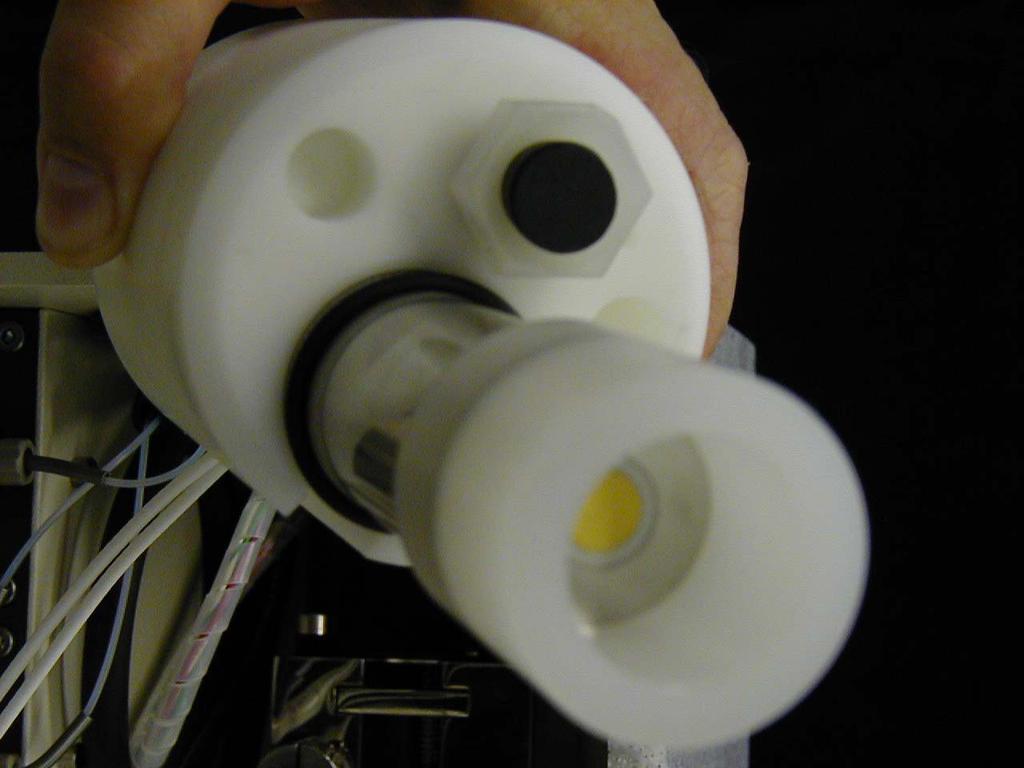
210 210

211 Zeta Probe with magnetic stirrer This setup is suitable for moderately concentrated systems with rather low viscosity. Stirring is important either for preventing sedimentation, or for proper mixing during titration. Two burettes titration block is shown on background. Injector of the burettes and other sensors could be placed into the hole in the holder plate next to the Zeta probe. 211

212 Zeta Probe with peristaltic pump. This setup is suitable for concentrated systems with rather high viscosity. It is especially important for systems that become strongly flocculated in the vicinity of isoelectricduring titration. Bottom block has cone shaped orifice for eliminated stagnation volumes. Sample is being pumped from the top to the bottom. Two burettes titration block is shown on background. Injector of the burettes could be placed into the hole in the holder plate next to the Zeta probe. 212

213 DT-100, Acoustic particle size sensor. The main purpose of this instrument is particle sizing. It can be also treated as high frequency longitudinal rheometer. We show here various setups just for this sensor. This instrument could contain, as options, temperature probe, ph probe, and 2 burettes titration. DT-100 with minimum sample volume This setup is suitable for stable systems only. It allows us to minimize sample volume down to 15 ml. 213

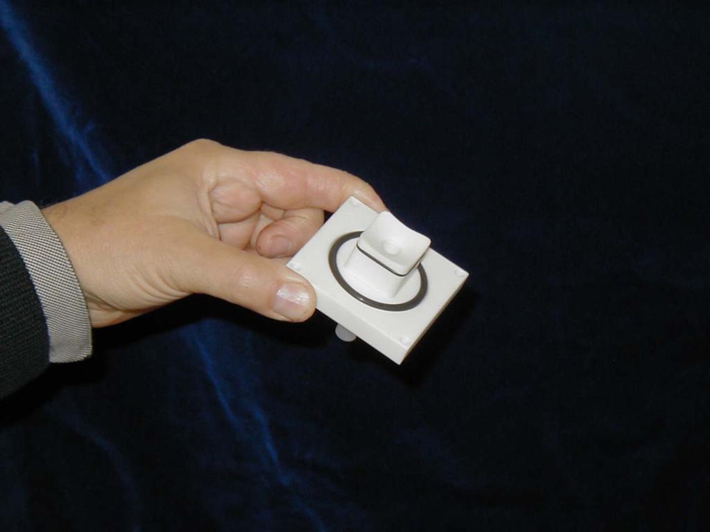
214 214

215 DT-100 with peristaltic pump This setup is suitable for viscose and unstable systems. Insert on the bottom of the sensor has cone shaped orifice for eliminated stagnation volumes. 215

216 DT-100 with magnetic stirrer This setup is suitable for moderately concentrated systems. Magnetic stirrer on the bottom of the sensor creates higher pressure there. This pressure pumps sample through the tube from bottom to the top. It is much more efficient than a simple vortex. Magnetic stirrer has a speed regulating knob at the bottom. We recommend using second position of the knob after first position when liquid starts moving. Magnetic cross could lose coupling at higher speeds. 216

217 DT-100 with titration setup This setup allows us connecting burettes to the acoustic sensor for running titration. Other sensors could be inserted into the bottom block. Port on the bottom of the bottom block could accommodate either magnetic stirrer or cone shaped connector for peristaltic pump. 217

218 DT-1200, Acoustic and Electroacoustic spectrometer. These instrument combines together all probes and titration. DT-1200 with magnetic stirrer This setup is suitable for moderately concentrated systems. Magnetic stirrer on the bottom of the sensor creates higher pressure there. This pressure pumps sample through the tube from bottom to the top. It is much more efficient than a simple vortex. Magnetic stirrer has a speed regulating knob at the bottom. We recommend using second position of the knob after first position when liquid starts moving. Magnetic cross could lose coupling at higher speeds. Sample volume is about 120 ml. 218

219 DT-1200 with peristaltic pump This setup is suitable for viscose and unstable systems. Insert on the bottom of the sensor has cone shaped orifice for eliminated stagnation volumes. Sample volume is 150 ml. 219

220 DT-1200, separate sensors This setup is suitable for stable systems. It allows us minimizing sample volume and simplifying cleaning. It is convenient also for making just PSD or just Zeta measurements. 220

221 DT-400, Titrator. This instrument makes ph titrations and ph-stat with concentrated systems. One of the purposes is monitoring milling. 221

222 DT-500, On-line sensor block. This is sensor block that could accommodate any combination of DTI sensors (Acoustic PSD, Electrosacoustic Zeta, conductivity, ph, temperature, dielectric permittivity). This block should be connected with the independent sample handling system to the process stream. 222

223 DTI additional sensors. Conductivity This probe is suitable only for aqueous solutions. 223

224 Dielectric permittivity Measurement mode. Plastic plug moved back. Liquid fills the space between electrodes. Cleaning mode. Plastic plug is moved forward and remove liquid from the inter electrodes space and clean electrodes. 224

225 Appendix A Setting up instrument for a specific customer There are several options that can be selected by the sales agent to tailor an instrument to be most useful to a particular customer. These options include three choices concerning the visibility of menu options from the Home page, namely: 1. Making menu to use Access database visible or not. 2. Making menu to use Material Wizard visible or not. 3. Making menu to use new Material Form visible or not. To access these options do following On Home page, click on LogIn/Out. The form to the right will open. If already logged in, then press Log Out button on this form, and then click LogIn/Out again on the Home page. In the box labeled User Name enter sales agent. In the box labeled Password enter and press Enter. Press Log In button. The form will close. On Home page, click on Tools Options. On Options window, click on Preferences tab. The last three items on the list allow you to make the choices described above. You can check or uncheck these in any combination. 225

226 When you are done, click on LogIn/Out on the Home page. On the form at right, select User Name as User. Enter password user and press Log In. The instrument is now set up for your customer. 226

227 Appendix B Retrieving Data from Database with a Query Note: Please see Addendum 1 which introduces the new Data View Form All measurements that you make will automatically be saved to a Microsoft Access database. The database consists of two files: c:\data_aco\data_aco.mdb and c:\data_aco\data_sys.mdb. File data_aco.mdb stores all measured data whereas file data_sys.mdb has stores all the Queries used to retrieve selected data. From the Home page, click on File - Database. The Microsoft Access form opens as depicted in Figure 0-1. Figure 0-1 Microsoft Access database main form The DT1200 uses two structures from Microsoft Access: Tables and Queries (There are also Forms, Reports, Macros, and Modules, but these are not used). 227

228 Click on the Table tab on the left edge of the database form. You will see the four tables used for saving data: Experiments, Materials, Measurements, and Samples The Material table stores information about the physical properties of the various materials you will be working with. Information on common materials is already stored in the database. If you work with a material which is not in the Material table, it is a simple matter to add this to the library. The Sample table stores the definition of each sample that you have defined when you entered information on the Home page before each measurement. The Measurement table stores all of the raw measured data and also the results of the analysis of that data. The Experiment table simply provides links between the Material, Sample and Measurement Tables. A single experiment may consist of many individual measurements. For example, a titration experiment may involve a series of measurements at various ph values. Normally you will not be concerned about these various tables. Instead, you will use Queries to retrieve whatever information you need. The necessary information from the Material, Sample, and Measurement Tables will be combined to show you all the information you need for any measurement or set of measurements that may be of interest. Click on the Query tab on the left edge of the database form. The list of Queries will appear similar to that shown in Figure

229 Figure 0-2 The Query list There are two types of Queries: Default Queries and User Queries. Default Queries are built-in and provided as a convenient way to retrieve standard sets of data. The name of all default queries starts with ~ and therefore appears at the beginning of the alphabetical list of Queries shown in Figure 0-2. These default queries are described in Table 1 229

230 . Table 1 Default Queries ~all records retrieves all records in data base ~past 30 days retrieves all measurements made during last 30 days ~Past 365 days retrieves all measurements made during last 365 days ~Past 7 days retrieves all measurements made during last 7 days ~Past 90 retrieves all measurements made during last 90 days ~Prototype this is used as a starting point for writing User Queries ~DemoQuery a query which gives typical examples, default for the Analysis Application or plotted with the Graphics Application. ~Today retrieves all measurements made today ~Yesterday & Today retrieves all measurements made yesterday and today Click on the Query ~Past 30 days. The measurement data obtained using this Query appears in the Select Query window as shown in Figure 0-3. Perhaps you will recognize some of the data that you obtained while going through the various lessons. Figure 0-3 Select Query window: ~Past 30 days 230

231 You can write additional User Queries to retrieve data of particular interest. Perhaps you want to make a set of graphs comparing a particular set of data. Writing a User Query is simple. You will simply modify an existing ~Prototype Query and then save it with a new name. In checking the Query list shown in Figure 0-2, you will see that there is no ~Prototype Query shown. Perhaps there is not one on your system either. It is easy to make one. We will simply save the Query ~Past 30 days with a new name, ~Prototype. Click on the menu item File Save Query as. The Save As form is displayed as shown in Figure 0-4. Figure 0-4 Saving Query as new name Enter the Query Name ~Prototype and click OK. The name at the top of the Select Query form changes to ~Prototype as shown in Figure 0-5 Figure 0-5 Data retrieved with ~Prototype Query Click on the Design button at the top of the database: form. The Select Query form changes to the Design View as shown in Figure 0-6. The Query is constructed by entering criteria for various fields in the database. The fields that can be compared against criteria are shown in the columns on the lower half of the Select Query form. The only criteria 231

232 used in the prototype is that the measurement date be larger than 30 days before the current date ( i.e. Date() 30 ) Figure 0-6 ~Prototype Query in Design View Let s say that we wanted our query to retrieve only data that met the following criteria: 1) the dispersed phase was silica or similar material 2) the weight fraction was greater than 5 % 3) the measurements were obtained sometime after Jan 1, 2003 We would then edit the query as follows: Since we want to see only data where the disperse phase was similar to silica we type alumina* in the criteria row of the disperse phase column. The * character is a wild card which means that any disperse phase which starts with silica will be retrieved with the Query. Since we want to see samples with weight fraction greater than 5% we type >5 in the criteria row in the column wt%. Since we want data obtained after Jan 1, 2003 we type >1/1/2003 in the criteria row for the measurement date column. The Query now should appear as shown in Figure 0-7. You might note that Silica* has been automatically edited to like Silica, and the format for the date has been changed somewhat, but this is of no concern to us. 232

233 Figure 0-7 User Defined Query to find silica slurries grater than 5 wt% measured since Jan 1, 2003 If you want to use other fields in specifying the data you wish to retrieve, you can simply add these fields to the list at the lower half of the Select Query form. To do this, click on the desired field in the data frame on the top half of the form, and drag it to any column position on the bottom half. For example, suppose you wanted to retrieve only data obtained at a temperature below 30 degrees C. Scroll down in the data frame until you locate Temp. Drag this field to some position on the lower half of the Select Query form and drop it. Then enter the >40 criteria in that column. The modified Select Query would then appear as shown in Figure

234 Figure 0-8 Adding additional fields to the Select Query When we have finished defining our Query we need to save it with a new name. Click on File Save as. The Save As dialog box opens, as shown in Figure 0-9. Type in your new query name and click on OK Figure 0-9 Saving modified prototype query to new name 234

235 Click on the top of the database form. Scroll down the list of Queries and you will see my new query that you just created. Click on Open to look at the records that have been retrieved. The Access form should now appear similar to Figure 0-10 Figure 0-10 Data retrieved with my new query 235