Product and Inventory Management (35E00300) Forecasting Models Trend analysis

Size: px

Start display at page:

Download "Product and Inventory Management (35E00300) Forecasting Models Trend analysis"

Jasper Gibson
6 years ago
Views:

1 Product and Inventory Management (35E00300) Forecasting Models Trend analysis

2 Exponential Smoothing Data Storage Shed Sales Period Actual Value(Y t ) Ŷ t-1 α Y t-1 Ŷ t-1 Ŷ t January 10 = February *( ) = March *( ) = April *( ) = May *( ) = June *( ) = July *( ) = August *( ) = September *( ) = October *( ) = November *( ) = December *( ) =

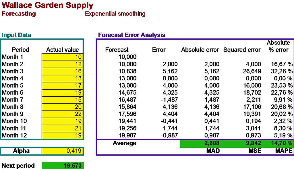
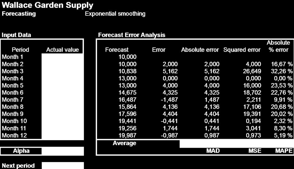
3 Exponential Smoothing (Alpha =.419) 3

4 Exponential Smoothing Exponential Smoothing Sheds Actual value Forecast January February March April May June July August September October November December 4

5 Forecasting Seasonal Data: Quick Method Enrolment (in thousands) Quarter Year 1 Year 2 Fall Winter Spring Summer Total Calculate average demand for each quarter or "Season" Year 1: 80/4 = 20 Year 2: 84/4 = 21 5

6 Forecasting Seasonal Data: Quick Method Compute a seasonal index for every season of every year for which you have data Enrolment (in thousands) Quarter Year 1 Year 2 Fall 24/20= 1,2 26/21= 1,238 Winter 23/20= 1,15 22/21= 1,048 Spring 19/20= 0,95 19/21= 0,905 Summer 14/20= 0,7 17/21= 0,810 Calculate average sesonal index for each index Quarter Fall (1,2+1,238)/2= 1,219 Winter (1,15+1,048)/2= 1,099 Spring (0,95+0,905)/2= 0,927 Summer (0,7+0,81)/2= 0,755 6

7 Forecasting Seasonal Data: Quick Method Calculate the average deamand per seson for next year (Next years annual number of enrolments is 9000) 90000/4 = Multiply next years average seasonal demand by each seasonal index Quarter Average demand Index Forecast (students) Fall , ,57 Winter , ,21 Spring , ,07 Summer , ,14 7

8 Trend & Seasonality Trend analysis Technique that fits a trend equation (or curve) to a series of historical data points Projects the equation into the future for medium and long term forecasts. Typically do not want to forecast into the future more than half the number of time periods used to generate the forecast Seasonality analysis Adjustment to time series data due to variations at certain periods. Adjust with seasonal index - ratio of average value of the item in a season to the overall annual average value. Examples: demand for coal in winter months; demand for soft drinks in the summer and over major holidays 8

9 Linear Trend Analysis Midwestern Manufacturing Sales Scatter Diagram Actual value (or) Y Period number (or) X

10 Least Squares for Linear Regression Midwestern Manufacturing Least Squares Method Values of Dependent Variables Objective: Minimize the squared deviations! Time 10

11 Least Squares Method Y^ = a + bx Where Y^= predicted value of the dependent variable (demand) X = value of the independent variable (time) a = Y-axis intercept = Y - b* X b = Slope of the regression line = [ Y XY - n X X 2 _ 2 - n X ] 11

12 Linear Trend Data & Error Analysis Midwestern Manufacturing Company Forecasting Linear trend analysis Enter the actual values in cells shaded YELLOW. Enter new time period at the bottom to forecast Input Data Forecast Error Analysis Actual value Period number Absolute Squared Absolute Period (or) Y (or) X Forecast Error error error % error Year % Year % Year % Year % Year % Year % Year % Average % Intercept MAD MSE MAPE Slope Next period

13 Least Squares Graph 13

14 Quantitative Forecasting using Trend Extrapolation There are several tools available for using trend extrapolation to first plot a trend line to historical time-series data, and then extend this to future periods for the purpose of forecasting or predicting values for those periods. Some might be tempted to visually extend a trend line to future periods with a pencil on a printed graph, but algebraic techniques are more precise, more varied, and more powerful. 14

15 Quantitative Forecasting using Trend Extrapolation There are three general approaches to use algebraic techniques for trend line extrapolation. 1. Applying formulas to calculate a future period. 2. Make use of specialized functions within a spreadsheet program or another data analysis program. 3. Make use of a spreadsheet or data analysis program to construct a graph with a trend line, and to automatically extend that trend line to future periods. 15

16 Triple Exponential Smoothing 16

17 Holt-Winters (HW) method This method is used when the data shows trend and seasonality. To handle seasonality, we have to add a third parameter. A third equation is introduced to take care of seasonality. The resulting set of equations is called the Holt- Winters (HW) method after the names of the inventors. There are two main HW models, depending on the type of seasonality Multiplicative Seasonal Model Additive Seasonal Model The rest of the todays presentation focuses on these two models

18 Multiplicative Seasonal Model This model is used when the data exhibits multiplicative seasonality The multiplicative seasonal model is appropriate for a time series in which the amplitude of the seasonal pattern is proportional to the average level of the series, i.e. a time series displaying multiplicative seasonality. This section describes the forecasting equations used in the model along with the initial values to be used for the parameters. 18

19 Overview This model is used when the data exhibits Multiplicative seasonality. We assume that the time series is represented by the model yy tt = bb 1 + bb 2 tt SS tt + εε tt Where bb 1 is the base signal also called the permanent component bb 2 is a linear trend component SS tt is a multiplicative seasonal factor εε tt is the random error component 19

20 Length of the Season Let the length of the season be LL periods. The seasonal factors are defined so that they sum to the length of the season, i.e. SS tt = LL 1 tt LL If the trend component bb 2 (previous page) is deemed unnecessary, it may be deleted from the model. 20

21 Notations Used Let the current deseasonalized level of the process at the end of period T be denoted by RR TT. At the end of a time period t, let RR tt be the estimate of the deseasonalized level. GG tt be the estimate of the trend SS tt be the estimate of seasonal component (seasonal index) 21

22 Procedure for updating the estimates of model parameters Overall smoothing Smoothing of the trend factor Smoothing of the seasonal index 22

23 Overall Smoothing RR tt = yy tt + 1 RR SS tt 1 tt 1 + GG tt 1 where 0 1 is the first smoothing constant. Dividing yy tt by SS tt 1, which is the seasonal factor for period T computed one season (L periods) ago, deseasonalizes the data so that only the trend component and the prior value of the permanent component enter into the updating process for RR tt. 23

24 Smoothing the Trend Factor GG tt = ββ SS tt SS tt ββ GG tt 1 where 0 ββ 1 is the second smoothing constant. The estimate of the trend component is simply the smoothed difference between two successive estimates of the deseasonalized level. 24

25 Smoothing of the seasonal index SS tt = γγ yy tt / RR tt + 1 γγ SS tt LL where 0 γγ 1 is the Third smoothing constant. 25

26 Value of Forecast 1. Forecast for the next period The forecast for the next period is given by: yy tt = RR tt 1 + GG tt 1 SS tt LL Note that the best estimate of the seasonal factor for this time period in the season is used, which was last updated LL periods ago. 26

27 Value of Forecast 2. Multiple-step-ahead forecasts (for T < q) The value of forecast T periods hence is given by: yy tt+tt = RR tt 1 + TT GG tt 1 SS tt+tt LL 27

28 Initial Values for Model Parameters As a rule of thumb, a minimum of two full seasons (or 2L periods) of historical data is needed to initialize a set of seasonal factors. Suppose data from m seasons are available and let xx jj, jj = 1,2,, mmmm denote the average of the observations during the j th season. 1. Estimation of trend component 2. Estimation of deseasonalized level 3. Estimation of seasonal components 28

29 Initial Value for Trend Component Estimate the trend component by: GG 0 = yy mm + yy 1 mm 29

30 Initial Value for Deseasonalized Level Estimate the deseasonalized level by: RR 0 = xx jj 30

31 Initial Values for Seasonal Components Seasonal factors are computed for each time period t = 1,2, mmmm as the ratio of actual observation to the average seasonally adjusted value for that season, further adjusted by the trend; that is, SS tt = yy ii RR 0 the t index is the position of the period t within the season. 31

32 Country Greeting Cards Triple Exponential Smoothing quarte level trend seasonal. year r period sales k forecast '(R) (G) (S) error abs.error %error , , , ,75 55,25 1, ,64 518,33 63,37 0,84 193,36 193,36 43,6% ,39 579,64 62,51 0,72-31,39 31,39 7,6% ,23 636,33 60,06 0,63-88,23 88,23 22,2% ,87 690,45 57,57 1,67-234,87 234,87 20,5% ,06 752,14 59,30 0,92 68,94 68,94 9,9% ,24 819,67 62,76 0,84 117,76 117,76 16,9% ,74 896,61 68,72 0,81 179,26 179,26 24,3% ,64 966,36 69,15 1,70 34,36 34,36 2,1% , ,77 73,46 1,08 188,66 188,66 16,5% , ,59 75,72 0,92 90,54 90,54 8,7% , ,02 74,75 0,78-37,24 37,24 4,0% , ,76 74,75 1,70-0,40 0,40 0,0% ,67 BIAS= 40, ,78 LS= 0,050 MAD= 105, ,31 TS= 0,420 MSE= 18039, ,33 SS= 0,950 MAPE= 14,7% 32

33 sales forecast year, quarter, period 33

34 Additive Seasonal Model This model is used when the data exhibits additive seasonality. The additive seasonal model is appropriate for a time series in which the amplitude of the seasonal pattern is independent of the average level of the series, i.e. a time series displaying additive seasonality. This section describes the forecasting equations used in the model along with the initial values to be used for the parameters. 34

35 Overview This model is used when the data exhibits Additive seasonality. We assume that the time series is represented by the model yy tt = bb 1 + bb 2 tt + SS tt + εε tt Where bb 1 is the base signal also called the permanent component bb 2 is a linear trend component SS tt is a additive seasonal factor εε tt is the random error component 35

36 Notations Used Let the current deseasonalized level of the process at the end of period T be denoted by RR TT. At the end of a time period t, let RR tt be the estimate of the deseasonalized level. GG tt be the estimate of the trend SS tt be the estimate of seasonal component (seasonal index) 36

37 Overall Smoothing RR tt = yy tt SS tt LL + 1 RR tt 1 + GG tt 1 where 0 1 is the first smoothing constant. Dividing yy tt by SS tt LL, which is the seasonal factor for period T computed one season (L periods) ago, deseasonalizes the data so that only the trend component and the prior value of the permanent component enter into the updating process for RR tt. 37

38 Smoothing the Trend Factor GG tt = ββ SS tt SS tt ββ GG tt 1 where 0 ββ 1 is the second smoothing constant. The estimate of the trend component is simply the smoothed difference between two successive estimates of the deseasonalized level. 38

39 Smoothing of the Seasonal Index SS tt = γγ yy tt SS tt + 1 γγ SS tt LL where 0 γγ 1 is the third smoothing constant. The estimate of the seasonal component is a combination of the most recently observed seasonal factor given by the demand yy tt divided by the deseasonalized series level estimate RR tt and the previous best seasonal factor estimate for this time period. Since seasonal factors represent deviations above and below the average, the average of any L consecutive seasonal factors should always be 1. Thus, after estimating SS tt, it is good practice to renormalize the most recent seasonal factors such that tt ii=tt qq+1 SS ii = qq 39

40 Value of Forecast Forecast for the next period The forecast for the next period is given by: yy tt = RR tt 1 + GG tt 1 + SS tt LL Note that the best estimate of the seasonal factor for this time period in the season is used, which was last updated LL periods ago. 40

41 Thank you! 41

Forecasting. Copyright 2015 Pearson Education, Inc.

Forecasting. Copyright 2015 Pearson Education, Inc. 5 Forecasting To accompany Quantitative Analysis for Management, Twelfth Edition, by Render, Stair, Hanna and Hale Power Point slides created by Jeff Heyl Copyright 2015 Pearson Education, Inc. LEARNING