Searching for Brown Dwarf Companions

Transcription

1 Searching for Brown Dwarf Companions November 2008 Avril C. Day-Jones A report submitted in partial fulfillment of the requirements of the University of Hertfordshire for the degree of Doctor of Philosophy.

2 2

3 Abstract In this thesis I present the search for ultracool dwarf companions to main sequence stars, subgiants and white dwarfs. The ultracool dwarfs identified here are benchmark objects, with known ages and distances. The online data archives, the two micron all sky survey (2MASS) and SuperCOS- MOS were searched for ultracool companions to white dwarfs, where one M9±1 companion to a DA white dwarf is spectroscopically confirmed as the widest separated system of its kind known to date. The age of the M9±1 is constrained to a minium age of 1.94Gyrs, based on the estimated age of the white dwarf from a spectroscopically derived T eff and log g and an initial-final mass relation. This search was extended using the next generation surveys, the sloan digital sky survey (SDSS) and the UK infrared deep sky survey (UKIDSS), where potential white dwarf + ultracool dwarf binary systems from this search are presented. A handful of these candidate systems were followed-up with second epoch near infrared (NIR) imaging. A new white dwarf with a spectroscopic M4 companion and a possible wide tertiary ultracool component is here confirmed. Also undertaken was a pilot imaging survey in the NIR, to search for ultracool companions to subgiants in the southern hemisphere using the Anglo-Australian telescope. The candidates from that search, as well as the subsequent follow-up of systems through second epoch NIR/optical imaging and methane imaging are presented. No systems are confirmed from the current data but a number of good candidates remain to be followed-up and look encouraging. A search for widely separated ultracool objects selected from 2MASS as companions to Hipparcos main-sequence stars was also undertaken. 16 candidate systems were revealed, five of which had been previously identified and two new L0±2 companions are here confirmed, as companions to the F5V spectroscopic system HD and the M dwarf GD 605. The properties of HD120005C were calculated using the DUSTY and COND models from the Lyon group, and the age of the systems were inferred from the primary members. For GD 605B no age constraint could be placed due to the lack of information available about the primary, but HD120005C has an estimated age of 2-4Gyr. In the final part of this thesis I investigate correlations with NIR broadband colours (J H, H K and J K) with respect to properties, T eff, log g and [Fe/H] for the benchmark ultracool dwarfs, both confirmed from the searches undertaken in this work and those available from the literature. This resulted in an observed correlation with NIR colour and T eff, which is presented here. I find no correlation however with NIR colours and log g or [Fe/H], due in part to a lack of suitable benchmarks. I show that despite the current lack of good benchmark objects, this work has the potential to allow UCD properties to be measured from observable characteristics, and suggest that expanding this study should reveal many more benchmarks where true correlation between properties and observables can be better investigated. 3

4 4

5 Acknowledgments I would like to extend a thank you to all the people who have provided help and support throughout my Ph.D. no matter how large or small, your help was always appreciated. I firstly need to thank my supervisors David Pinfield, Hugh Jones and Ralf Napiwotzki for their constant support and help with every aspect of the Ph.D, for their patience and understanding and for teaching me the skills needed to succeed. I could also not have done this Ph.D. without the support, both emotionally and financially from all of my immediate and extended family. I also owe a very big thank you to James Jenkins, who helped me with many scientific and computing aspects throughout my Ph.D, as well as his tireless support, encouragement, motivation and constant belief in me throughout. I would also like to thank my fellow students and inhabitants of Starlink for their help, support and hundreds of cups of tea over the last 3 years, with a special thanks to Bob Chapman, Stuart Folkes, Douglas Weights and Krispian Lowe for all their many hours of help with IDL, IRAF and LATEX. I also extend a thank you to the staff and grad students at Penn State University, who made it possible for me to work there during the summer of 2008 and for the fantastic experience I had while I was there. I also owe thanks to Harriet Parsons, Simon Weston, Andy Gallagher and Joanna Goodger for providing a temporary roof and their sofas/floors for the last months of my write up. Thank You to you all! I would like to dedicate this thesis to my grandmother Joyceline Pay, who passed away during the last weeks of writing this thesis, I know she would have been proud to see it come to fruition. 5

6 6

7 Contents 1 Background Introduction Properties of brown and ultracool dwarfs Benchmark ultracool dwarfs Ultracool formation scenarios The ultracool IMF and birthrate The substellar initial mass function The substellar birth rate Ultracool evolution Understanding and interpretation of ultracool atmospheres Atmospheric models Benchmark UCDs as members of binary systems Stellar evolution beyond the main-sequence Motivation and thesis structure Selection Techniques Selecting white dwarfs White dwarfs in SuperCOSMOS White dwarfs in SDSS Selecting ultracool dwarfs L dwarfs in 2MASS L and T dwarfs in UKIDSS

8 3 Ultracool companions to white dwarfs Selecting candidate binary pairs Searching SuperCOSMOS and 2MASS Proper motions of candidate systems A wide WD + UCD binary Spectral classification of UCDc-1: 2MASSJ Spectral classification of WDc-1: 2MASSJ A randomly aligned pair? Binary age UCD properties Searching SDSS and UKIDSS Simulated numbers of WD + UCD binaries Binary selection Candidate WD + UCD systems Second epoch imaging and proper motion analysis of candidate UCDs A candidate wide L dwarf companion to a spectroscopic WD + M dwarf binary Summary of chapter Ultracool companions to Subgiants A pilot survey of southern Hipparcos subgiants Selection of subgiants Simulated populations The pilot survey Observing strategy Extraction and calibration of photometry Selection of good candidate systems Follow-up Observations Second epoch imaging Methane imaging Discussion

9 5 Ultracool companions to main-sequence stars Selection of Hipparcos main-sequence + UCD wide binary systems Spectroscopic follow-up observations Reduction and extraction of data Spectral classifications Cand Cand Parameters of the systems Gl HD Discussion Further discussion and conclusions The ultracool mass-age distribution The current benchmark population Open clusters and moving groups UCDs in binaries Field UCDs Discussion The effects of gravity and metallicity on observed UCD properties Correlations with colour and physical properties Future Work

10 10

11 List of Figures 1.1 Optical spectra of an M9, L3 and L8 types from Kirkpatrick et al. (1999) NIR spectra of M7-L2 dwarfs from Reid et al. (2001) NIR spectra of L3.5-L8 dwarfs from Reid et al. (2001) NIR spectra of T dwarfs from Burgasser et al. (2003) Main-sequence mass function from Miller & Scalo (1979) Pleiades mass function from Lodieu et al. (2007) Bolometric luminosity functions from Allen et al. (2005) Comparison of Φ(T eff ) for different birth rate scenarios from Burgasser et al. (2004) Cooling tracks for brown dwarfs, stars and planets taken from Burrows et al. (1997) Hertzsprung-Russell diagram Cooling tracks for DA WDs from Chabrier et al. (2000) The initial-final-mass-relation for WDs from Dobbie et al. (2006) A reduced proper motion diagram of WD candidates from SuperCOSMOS A reduced proper motion diagram of WDs from SDSS DR2 from Kilic et al. (2006) A u g against g r two colour diagram of WDs selected from SDSS (DR6) A J H against H K two colour diagram of L dwarfs from dwarfarchives.org A Y J against J H two colour diagram showing L and T dwarf selection regions A WD M B against B R absolute colour-magnitude diagram for McCook & Sion (1999) WDs with known parallax Separation area probed by 2MASS and SuperCOSMOS for WD + UCD binaries

12 3.3 An M J against J K absolute colour-magnitude diagram showing companion UCD candidates SuperCOSMOS and 2MASS images show UCDc-1 (2MASSJ ) and WDc-1 (2MASSJ ) J- band spectra of UCDc-1 (2MASSJ ) H- band spectra of UCDc-1 (2MASSJ ) Optical spectrum of the confirmed white dwarf WDc-1 (2MASSJ ) Model atmosphere fit to the Balmer lines of 2MASSJ Simulated WD + UCD J- against g- magnitude diagram from Pinfield et al. (2006) A WD M g against g r colour-magnitude diagram for McCook & Sion (1999) WDs with known parallax A UCD colour-magnitude diagram for L and T dwarfs with known parallax from dwarfarchives.org Left: i z against spectral type relation. Right: z J against spectral type relation from Hawley et al. (2002) Colour-colour relations for M, L and T dwarfs from Hawley et al. (2002) Left: A Y J against J H two-colour diagram. Right: An M J against J H CMD of UCD candidate components of potential wide WD + UCD binaries A u g against g r two colour diagram showing WD candidate components of potential wide WD + UCD binaries SDSS spectra of the WD candidate nbin Model DA4 WD SDSS spectra combined with M0-L0 spectra Model DA5 WD SDSS spectra combined with M0-L0 spectra Model DA4 WD SDSS combined with an M4 spectra M4 component of the convolved spectra of nbin Subgiant selection.(a) An M V against B V diagram of Hipparcos stars with V < 13.0 and π/σ 4. (b) Theoretical isochrones from Girardi et al. (2000) for solar metallicity Simulated distance - magnitude distribution of UCD companions to Hipparcos subgiants from Pinfield at al. (2006) Predicted separation-distance distribution of subgiant + UCD binaries A diagram showing the imaging strategy used for the subgiant survey on AAT/IRIS An airmass curve for standard star observations

13 4.6 A J H against magnitude plot showing the zero point calibration using 2MASS objects for the J- band for one IRIS2 imaging field A plot of magnitude against the difference in flux between two aperture sizes in the J- band for objects in one image A J H against Y J two-colour diagram, showing the position of main sequence stars, M, L and T dwarfs Left: A J H against Z J two-colour diagram, showing candidate L and T dwarfs. Right: A M J against J H CMD of L and T dwarf candidates Plot from Tinney et al. (2005) showing the position of the methane filters; CH 4 s and CH 4 l A CH 4 s CH 4 l colour against spectral type plot from Tinney et al. (2005) A CH 4 s CH 4 l against CH 4 s CMD for Cand T Top: M J against J K CMD for candidate L dwarf companions to Hipparcos stars. Bottom: A distance - separation plot for the candidate mainsequence + L dwarf binary systems A vector point diagram of four candidate main sequence + L dwarf common proper motion systems The ZJ spectrum of Cand The HK spectrum of Cand The HK spectrum of Cand The ZJ spectrum of Cand 13 overplotted with template spectra (M7, M8, M9, L0.5, L1 and L2 type) from Cushing, Rayner & Vacca (2005) The HK spectrum of Cand 13, overplotted with template spectra (M7, M8, M9, L0.5, L1 and L2 type) from Cushing, Rayner & Vacca (2005) The HK band spectrum of Cand 10, overplotted with template spectra (M7, M8, M9, L0.5, L1 and L2 type) from Cushing, Rayner & Vacca (2005) Simulations of the UCD mass-age population from Pinfield et al. (2006) for 2MASS and UKIDSS Simulations of the UCD mass-age population from Pinfield et al. (2006) for UCD companions to WDs and subgiants The mass-age distribution of benchmark UCDs from the literature and both confirmed and candidate objects presented in this work T eff against log g for benchmark UCDs taken from the literature and both confirmed and candidate objects presented in this work T eff against Fe/H for benchmark UCDs taken from the literature and both confirmed and candidate objects presented in this work

14 6.6 M J against J K colour space showing the dependence of metallicity and gravity on models from Burrows et al. (2006) for their COND and DUSTY models T eff against J K space predictions of the DUSTY and COND models from Burrows et al. (2006) Left: M J as a function of spectral type and Right: M J as a function of J K colour for L and T dwarfs from Knapp et al. (2004) T eff against colour plot of benchmark L dwarfs with NIR J H, H K and J K colours T eff against colour plot of benchmark T dwarfs with NIR J H, H K and J K colours Colour against log g, where the colour-t eff trend has been subtracted from the colour, for benchmark L dwarfs with NIR J H, H K and J K colours Colour against log g, where the colour-t eff trend has been subtracted from the colour, for benchmark T dwarfs with NIR J H, H K and J K colours Colour against Fe/H, where the colour-t eff trend has been subtracted from the colour, for benchmark L dwarfs with NIR J H, H K and J K colours Colour against Fe/H, where the colour-t eff trend has been subtracted from the colour, for benchmark T dwarfs with NIR J H, H K and J K colours Improved T eff against colour plot, where the effects of log g and Fe/H have been removed for the benchmark L dwarfs with NIR J H, H K and J K colours

15 List of Tables 1.1 The classification scheme for WDs from Sion et al. (1983) Galactic co-ordinates of contaminated and overcrowded regions removed Candidate UCD + WD binary systems from SuperCOSMOS and 2MASS Estimated spectral types for 2MASSJ Fit results and derived quantities for WD mass, cooling age and absolute magnitude for 2MASSJ Parameters of the binary 2MASSJ MASSJ and its components Parameters of the WD component of the WD + UCD binary candidates with optical counterparts selected from SDSS and UKIDSS Parameters of the UCD component of the WD + UCD binary candidates with optical counterparts selected from SDSS and UKIDSS Parameters of the WD component of the WD + late M dwarf binary candidates selected from SDSS and UKIDSS Parameters of the UCD component of the WD + late M dwarf binary candidates selected from SDSS and UKIDSS Parameters of the WD component of the WD + UCD i- band drop out binary candidates selected from SDSS and UKIDSS Parameters of the UCD component of the WD + UCD i- band drop out binary candidates selected from SDSS and UKIDSS Parameters of the WD component of the WD + UCD non-optical detection binary candidates selected from SDSS and UKIDSS Parameters of the UCD component of the WD + UCD non-optical detection binary candidates selected from SDSS and UKIDSS Proper motion analysis for followed up candidate WD + UCD binary pairs from SDSS and UKIDSS Candidate subgiant + UCD binary systems

16 4.2 Proper motion measurements of candidate L and early T dwarfs The status of UCD candidates (confirmed or not) Widely separated main sequence + L dwarf candidate systems Spectral ratios for Cand Equivalent widths for Cand Spectral ratios for Cand Parameters of the system HD Subgiant + UCD candidates with age and mass constraints estimated from the Lyon group DUSTY and COND models Main-sequence + UCD Candidates with known ages and masses derived from the Lyon group DUSTY and COND models Cluster and Moving Group UCDs Pleiades cluster UCDs UCD in binaries UCD + WD binaries Field UCDs with age estimates Parameters of fitting equations for colours of T dwarfs Parameters of fitting equations for colours of L dwarfs

17 Chapter 1 Background. In this chapter the background knowledge relevant to the later chapters in this thesis is discussed. In brief the main topics here include an overview of the understanding and interpretation of ultracool dwarf (UCD) and brown dwarf (BD) atmospheres, formation scenarios, the ultracool contribution to the initial mass function and the birth rate of L and T dwarfs are also discussed in context. A particular emphasis is given to benchmark UCDs, why they are needed, how they will be used and where they can be found. 1.1 Introduction In just over a decade nearly 700 UCDs have been discovered since those that were first confirmed (Tiede 1 (M8); Rebolo, Zapatero-Osorio & Martin 1995 and Gliese 229B (T6.5); Nakajima et al. 1995). This is in large thanks to the rise of deep large area surveys such as the Two Micron All Sky Survey (2MASS), the Sloan Digital Sky Survey (SDSS) and more recently the UK Infrared Deep Sky Survey (UKIDSS). These populations have helped shape the understanding of ultracool dwarfs and extended the classification system for substellar objects including the creation of two new spectral types L and T. The latest M dwarfs ( M7-9) have effective temperature (T eff ) reaching down to 2300K. At lower T eff ( K) are the L dwarfs, which have very dusty upper atmospheres and generally very red colours. T dwarfs are even cooler having T eff in the range K, where the low T eff limit is currently defined by the recently discovered T8+ dwarfs, ULAS J (Warren et al. 2007), CFBDS J (Delorme et al. 2008) and ULAS 17

18 1335 (Burningham et al. 2008). T dwarf spectra are dominated by strong water vapour and methane bands, and generally appear bluer in the near infrared (NIR) (Geballe et al. 2003; Burgasser, Burrows & Kirkpatrick 2006). The physics of ultracool atmospheres is complex and very difficult to accurately model. Atmospheric dust formation is particularly challenging for theory (Allard et al. 2001; Burrows, Sudarsky & Hubeny 2006) and there are a variety of other important issues that are not well understood, including the completeness of CH 4 /H 2 O molecular opacities, their dependence on T eff, gravity and metallicity (e.g. Jones et al. 2005; Burgasser et al. 2006; Liu, Leggett & Chiu 2007), as well as the possible presence of vertical mixing in such atmospheres (Saumon et al. 2007). The emergent spectra from ultracool atmospheres are likely strongly affected by factors such as gravity and metallicity (e.g. Knapp et al. 2004; Burgasser et al. 2006; Metchev & Hillenbrand 2006), which highlights the need for an improved understanding of such effects if physical properties (e.g. mass, age and composition) are to be constrained observationally (e.g. spectroscopically). Discovering UCDs whose properties can be inferred indirectly (without the need for atmospheric models) is an excellent way to provide a test-bed for theory and observationally pin down how physical properties affect spectra. Such UCDs are referred to as benchmark objects (e.g. Pinfield et al. 2006). A population of benchmark UCDs with a broad range of atmospheric properties will be invaluable in the task of determining the full extent of spectral sensitivity to variations in UCD physical properties. However, such benchmarks are not common and the constraints on their properties are not always particularly strong Properties of brown and ultracool dwarfs BDs were first theorised by Kumar (1963) as a cool extension of the main-sequence, beyond the M7 type. They are not massive enough to ignite or burn hydrogen in their core, such that an upper mass limit would correspond approximately to 0.075M (Chabrier et al. 2000a), although it is possible for this limit to change with metallicity (if the BD is metal poor then it can have a larger mass). The lower end of the mass limit remains ill defined approaching the planetary mass regime. The difference between BDs and giant planets is commonly assumed to be the way in which they form. It was originally suspected that BDs form in the same way as stars, from the fragmentation of a gas cloud (as shown by the simulations of Bate 1998) and that giant planets form via accretion onto rocky cores 18

19 in a proto-planetary disk (e.g. Pollack et al. 1996). However the formation mechanisms for both types of object are not fully understood. The currently adopted lower mass limit is taken from the deuterium burning minimum mass (0.013M ), which draws the distinction that all BDs burn deuterium at some point during their lifetime. However Bate (2005) showed that the minimum mass (i.e. the deuterium burning limit) of a BD can change by 3-9 M Jup from simulating clouds where the opacity limit is set by the clouds metallicity, such that metallicity can drive this mass up towards 0.015M. This has also been challenged more recently by the discovery of planetary mass objects in Orion (Lucas et al. 2006; Weights et al. 2008) and 2MASS1207B, an 8±2M Jup L dwarf (Mohanty et al. 2007). For ages of a few Gyr, these masses correspond to temperatures generally less than 2300K (Kirkpatrick et al. 1999b) encompassing two new spectral classifications, the L and T dwarfs (Kirkpatrick et al. 1999b; Martín et al. 1999). Traditionally spectral typing is done using optical spectra as is typically done for L dwarfs, following the conventions of Kirkpatrick et al. (1999b). However, as L dwarfs are faint at these wavelengths it is often easier to use NIR spectra. Indeed T dwarfs are very faint in the optical and are thus formally classified in the NIR following the classification scheme of Burgasser et al. (2006). In general L and T dwarfs are BDs but objects later than M7 can be referred to as UCDs. From an M dwarf a UCD is expected to cool and evolve through the L to the T dwarf sequence and to cooler temperatures (Kirkpatrick et al. 1999b). L dwarfs L dwarfs have temperatures between K, such that the peak of their flux is more red-ward than main-sequence stars. Their spectra tend to exhibit strong H 2 O absorption, along with metal-oxide (TiO and ViO), metal (CaH and FeH) and alkali band (Na, K, Cs, Rb) features, which along with the effects of low temperature cause opacities which redden their colours. GD 165B, a companion to a white dwarf (Becklin & Zuckerman 1988) is often taken as the prototype L dwarf. Shown in Fig. 1.1 is an example of the spectra of late M through to L dwarfs at optical wavelengths, highlighted are some of the identifying features specifically of L dwarfs, including water vapour and alkali metal lines. Fig 1.2 and 1.3 show the NIR spectrum of late M and L dwarfs, where it can clearly be seen that for later L types the spectra around 1.5 µm becomes much more enhanced. 19

20 Figure 1.1: Optical spectra of an M9, L3 and L8 type, showing water vapour and alkali metal features from Kirkpatrick et al. (1999). 20

21 6 LP M7 LP M8 4 2M0345 L0 2M0746 L M0829 L2 2M1029 L Figure 1.2: NIR spectra of M7-L2 dwarfs from Reid et al. (2001). The shaded regions show areas affected by terrestrial water vapour absorption. Refer to Figs. 1.1 and 1.4 for spectral features. 5 2M0036 L M1112 L4.5 3 D0205 L7 2 2M0825 L M0310 L Figure 1.3: NIR spectra of L3.5-L8 dwarfs from Reid et al. (2001). The shaded regions show areas affected by terrestrial water vapour absorption. Refer to Figs. 1.1 and 1.4 for spectral features. 21

22 Figure 1.4: NIR spectra of T dwarfs from Burgasser et al. (2003). T dwarfs T dwarfs are cooler than Ls, with a typical range in temperature of K or cooler (Burningham et al. 2008), where their spectra become dominated by CH 4 absorption. At these temperatures the FeH bands seen in L dwarfs disappear. T dwarfs develop much bluer NIR colours as the dust layers present themselves below the photosphere, such that the effects of dust reddening in L dwarfs no longer occur. Also noticeable is the strong absorption of H 2 O and CH 4. Like GD 165B, Gl 229B, one of the first confirmed BDs is taken as the prototype T dwarf. Examples of T dwarf spectra are shown in Fig. 1.4, where the H 2 O and CH 4 features are indicated. These spectral classifications are further split into sub-classes of L0-L9 and T0-T9. These classifications are based mainly on the strength of the CH 4 and H 2 O absorption and employ flux comparisons to determine a dwarfs position within the sub-classification scheme. Band passes of determined widths are centred on features of interest and regions of slope, their integrated fluxes determined and then compared with relations between these bandpass flux estimates of known spectral type, e.g. Geballe et al. (2003) use four regions in the NIR spectra, centred at 1.15 and 1.50µm (H 2 O features) and

23 and 2.20µm (CH 4 features). More recently other features such as FeH are also used to generate more accurate relations within the L and T sub-classes (Slesnick, Hillenbrand & Carpenter 2004). Another method is to use the equivalent widths of the potassium lines at 1.18µm (Reid et al. 2001a). For the very late T dwarfs that are now being discovered (ULAS J Warren et al and CFBDS J Delorme et al. 2008) a further spectral class beyond T will be needed. Pre-emptively coined Y-dwarfs by Kirkpatrick et al. (1999b) they are expected to be characteristically different from T dwarfs. Such changes may result from the emergence of ammonia absorption in the NIR, or effects due to the condensation of water clouds at 400K (similar to those seen in Jupiter). 1.2 Benchmark ultracool dwarfs There is no official criteria for what constitutes a benchmark UCD in the literature, other than the fact that it has some known properties. In the context of this thesis however, benchmark UCDs are those that have a known age. This parameter is vitally important for the understanding of UCD properties and how they evolve with time. Currently it is not possible to calculate the age of an isolated UCD in the field (with the exception of very young objects that show lithium in their spectra) as models are not yet robust enough for this prediction. Benchmark UCDs are thus vital to the calibration of such models and are likely to be the testbeds for interpreting UCD atmospheric effects, which could lead to the accurate prediction of physical properties from observable characteristics. Potentially a UCD with an indicated age constraint is likely to be useful, when considering overall trends. These are discussed in the later chapters of this thesis, where all known UCDs with an age estimate are presented. However, if the age of the UCD is not very accurate then the associated properties may not be particularly useful for calibrating models. The ideal benchmark UCD should have an age accurate to 10% (Pinfield et al. 2006). These benchmarks are the subject of the searches in this thesis. Where such benchmarks may be found, as well as the application for the use of such benchmarks are described in the following sections. 23

24 1.2.1 Ultracool formation scenarios The formation of UCDs is still not well understood, but it is likely that they form initially like stars (core collapse and accretion) but never acquire enough mass to ignite stable hydrogen burning, only burning deuterium for a limited period of time, such that their formation may take a slightly different course to those of normal stars. Briefly described here are the four main types of theorised formation mechanisms, these include formation by turbulent fragmentation, disc fragmentation, photo-erosion and ejection. Turbulent Fragmentation Formation of UCDs via turbulent fragmentation was first proposed by Padoan & Nordlund (2002), who suggested that very low-mass cores could be formed during the process of fragmentation in a turbulent cloud, which would then go on to produce very low-mass objects. Their simulations show that turbulent flows commonly gives rise to variations in the mass density distribution allowing substellar mass cores to be dense enough to collapse and form UCDs. Disk Fragmentation It may also be possible for UCDs to form from initially massive prestellar cores via fragmentation of a large circumstellar disk (Bate, Bonnell & Bromm 2003). Whitworth & Goodwin (2005) state that this theory could be possible for large disks ( 1000AU) where the separation between the two components is relatively large ( 100AU), but would not work for stars with smaller disks, where the temperature and surface density are higher, such that the photo-fragments (small forming cores) are unable to cool fast enough to condense out to form a UCD in the disk. This formation mechanism may also explain the brown dwarf desert (the observed trend where UCDs are not found at separations of < 5AU from a main-sequence star binary companion Grether & Lineweaver 2006) as UCDs formed in this fashion must have large separations. Whitworth & Stamatellos (2006) also support this theory of formation but suggest that a massive enough circumstellar disk is likely to be rare and short-lived, converting into UCDs quickly on a dynamical timescale of only 10 4 yr. 24

25 Ejection The theory of UCD formation through embryo ejection or liberation was first suggested by Reipurth & Clarke (2001). They postulated that UCDs form from prestellar cores that are ejected from dynamically interacting multiple systems before they have had time to accrete enough mass to ignite hydrogen. UCDs formed in this manner would exhibit no kinematic imprint and are likely to be found as isolated objects, as shown in the simulations of Bate et al. (see This formation mechanism also requires a large amount of initial formation by fragmentation and core collapse to produce the protostellar embryo that is ejected from the system. It cannot however explain the large number of close UCD binaries that have been observed (Pinfield et al. 2003). Photo-erosion The fourth formation mechanism is the theory of photo-erosion, whereby UCDs form in the presence of a higher mass star embedded in a HII region. The higher mass object causes compression waves and an ionisation front that photo-erodes surrounding low mass cores. This theory produces UCDs for a wide range of initial conditions and predicts close UCD binaries. However, the process is inefficient as it requires a massive protostellar core to be eroded to form a single UCD, and can only work in the presence of an OB type star to produce the high levels of UV needed for this formation mechanism to work (Whitworth & Goodwin 2005). None of the methods outlined here can, by themselves predict all the observed dynamics of UCDs (the numbers of isolated and both close and wide binary systems) and it seems likely that a combination of these mechanisms is responsible for at least some of the UCDs discovered to date, possibly being dependent on environment, epoch and metallicity, as reflected by collective UCD properties that are seen by observations. Indeed Goodwin & Whitworth (2007) favour a combination of formation scenarios, suggesting that UCDs are initially binary companions formed by gravitational fragmentation of the outer parts (R > 100 AU) of the protostellar disc of a low-mass hydrogen-burning star. These are then gently disrupted by passing stars, rather than violent interaction as suggested by Reipurth & Clarke (2001). UCDs formed in this way would have velocity dispersions and spatial distributions similar to that of higher-mass stars and they would likely be able to retain discs and sustain accretion and outflows. This also implies that most stars 25

26 and UCDs should form in binary or multiple systems, which is supported by observations (Pinfield et al. 2003), thus studies of UCDs in binaries could potentially be revealing about their formation mechanisms. 1.3 The ultracool IMF and birthrate To fully understand the nature of UCDs (other than the treatment of dust) and their contribution to the galaxy, there are several important factors that need to be understood in order to answer these questions. How do they form? at what rate does this happen? how do they evolve? and what is their contribution to the very low mass end of the mass function (MF) and the initial mass functions (IMF)? The current knowledge on these factors are briefly outlined below The substellar initial mass function The IMF describes the distribution of newly formed stars as a function of mass, which can be described as a power law of the form M α. Salpeter (1955) showed that α=2.35 for stars equal to or larger than M, this is referred to as the Salpeter function and states that the number of stars of each mass range decreases with increasing mass. This form of the IMF stays fairly uniform regardless of environment for stars M>M. Miller & Scalo (1979) and Scalo (1986) expanded on this work for stars < M, suggesting that the IMF flattens for lower masses where α=0 for stars below M, as shown in Fig Kroupa (2001) however suggests that α=2.3 to half a solar mass but then reduces to α=1.3 for masses 0.5<M <0.08 and to α=0.3 below 0.08M. Traditionally the IMF is estimated from a luminosity function and a mass-luminosity relation, this is a problem however for UCDs, as the initial heat from gravitational contraction is slowly radiated away with time, such that the UCD mass-luminosity relation is a factor of age. Currently neither the mass, nor the age can be calculated from luminosity alone, making it difficult to calculate an IMF for field UCDs, as a history of the star formation along with an accurate age is needed. This was attempted by Reid et al. (1999), who calculated an IMF for stars in the solar neighbourhood from 2MASS and showed evidence for a substellar IMF that is shallower than the Salpeter IMF. However the models they use (Burrows et al. 1997b) are geared towards dust-free atmospheres and do not represent the characteristics of dustier 26

27 Figure 1.5: The present day mass function of main-sequence field stars from Miller & Scalo (1979), where the MF φ ms (log M) as the number of stars (pc 2 logm). L dwarfs. Allen et al. (2005) took a slightly different approach and calculated the IMF for M<0.08M to be in the range -0.6< α <0.6 using Bayesian techniques. The problems associated with determining the IMF for field UCDs could potentially be solved by determining the ages of UCDs and obtaining theoretical masses using evolutionary models. This may be done by observing open cluster populations where stars and UCDs of different masses with well defined ages would be abundant. There are however potential difficulties when observing objects in clusters such as sources of extinction, uncertainties in age and distance, and contamination from non-members. Studies of young clusters have been performed by Andersen et al. (2008) who looked at the IMF in young clusters including IC348, where Luhman et al. (2003b) found that the IMF rises as a Salpeter function from high/intermediate masses down to M and then rises more slowly to a mass around M= M, turning over and declining into the substellar regime. They also looked at the IMF in Taurus (Briceño et al. 2002, Luhman et al. 2003a) and find that it appears to rise quickly to a peak of 0.8M and then steadily declines to lower masses. The trend of a falling mass function in the ultracool regime is generally shared with the observations in other clusters (Chameleon1; Luhman 2007, Pleiades; Lodieu et al. 2007a; Chabrier 2003; Moraux et al. 2003, Orion; Hillenbrand 1997; Luhman et al. 2000; Muench et al and NGC2024; Levine et al. 2006) as can be seen in Fig. 1.6, showing the MF of the Pleiades (Lodieu et al. 2007a). The different 27

28 forms of the IMF in these clusters all show subtle differences, suggesting that they might be sensitive to initial condition. These differences however, may also be able to help pin down the formation mechanisms for UCDs. The recent simulations and studies of late T dwarfs (>T4) in the field from the UKIDSS LAS by Pinfield et al. (2008) suggest that a log normal form of the MF agrees best with both their observations and observations of clusters (e.g. Pleiades MF from Chabrier 2003; Lodieu et al. 2007a). The slope of the function appears to steepen, increasing as mass decreases, suggesting a function that is consistent with an α=0 power law around a mass of 0.04M. This would also suggest that as T dwarfs probe lower mass ranges, the mass function may differ for L dwarfs from that of T dwarfs and that T dwarfs may be more sensitive to changes in the IMF, as shown by the simulations of Allen et al. (2005) in Fig The findings of Pinfield et al. (2008) indicate that for the field population the substellar MF is most consistent with an α=-1.0 and α=0.0 for L and T dwarf populations, respectively The substellar birth rate The birth rate is the number density of stars born per unit time and determines the MF and IMF. For main-sequence stars the MF is thought to stay constant with time (Miller & Scalo 1979) but remains undefined for substellar objects. Burgasser (2004) made Monte Carlo simulations of five UCD birth rate scenarios, including a constant birth rate (flat), similar to that taken for galactic star formation, an exponential birth rate, such that the star formation rate scales with average gas density. They also consider an empirical birth rate in the form of a series of star formation bursts, which would agree with the apparent increase in star formation 400 Myr ago (Barry 1988). A fourth scenario is a stochastic birth rate, where star formation occurs only in young clusters and only for a series of shortlived bursts, producing an equal amount of UCDs at each event. Finally they consider a halo birth rate where only UCDs born over a 1 Gyr range, occurring 9 Gyr ago and that represent the halo population. These five scenarios are all compared for α=0.5, where they shows that there is little difference between the majority of scenarios and that only the extreme exponential and halo birth rates show any strong dissimilarities, as these scenarios produce a larger number of older, more evolved UCDs. They also suggest that UCDs in the T eff range K (L and early T dwarfs) may be more sensitive to the birth rate than later type T dwarfs, as shown by Fig Using a number of late T dwarfs 28

29 Figure 1.6: Left: The Pleiades mass function from Lodieu et al. 2007a of UKIDSS GCS DR1. The solid lines show segments of a best fit power law where α=0.98 ± 0.87 for M (filled stars),α=-0.18 ± 0.24 for M (open triangles) and α= ± 1.20 for M (open squares). Right: A plot of α for the Pleiades mass function, showing the power law fits from different studies. The filled circles are from Lodieu et al. 2007a, open squares from Moraux et al. 2003, open triangles from Tej et al and open diamonds from Martín et al The solid line shows the studies from Lodieu et al. 2007a, dashed lines are from studies by Hambly et al and dot-dashed line from Deacon & Hambl

30 Figure 1.7: Three bolometric luminosity functions from Allen et al. (2005) comparing models of α = 0.0 (solid line), 0.5 (dotted line) and 1.0 (dot-dashed line) for M, L and T dwarfs. discovered from the UKIDSS LAS, Pinfield et al. (2008) suggest from observations that an IMF of the form α 0 is unlikely and favour a range of -1.0<α<-0.5. Analysis of a larger sample of L and early T dwarfs, over short T eff =100K bins in the range K, would be able to rule out at least extreme scenarios (e.g. exponential or halo birth rates) Ultracool evolution BDs and UCDs are not massive enough to burn hydrogen, but instead burn deuterium for some fraction of their lifetime. For the most massive UCDs this can be as short as 10Myr, at which point deuterium burning within the core will cease and the UCD will be supported by electron degeneracy pressure. They then simply cool and radiate away their internal thermal energy. Fig. 1.9 shows the cooling tracks for low-mass stars, brown dwarfs and exoplanets, taken from Burrows et al. (1997a). UCDs have masses between those of low-mass stars and exoplanets and as a result their cooling tracks appear like a mixture of the two cases. The kinks in the tracks for the higher mass objects relate to the switch-off of deuterium burning in the particular type of object. It is clear that 30

31 Figure 1.8: Comparison of Φ(T eff ) for α=0.5 for different birth rate scenarios from Burgasser et al. (2004) as disussed in the text. These include a flat/constant (solid black line), exponential (gray solid line), empirial (black dtted line), a stocastic/cluster (gray dotted line) and a halo (black dashed line) birth rate. The constant, empirical and cluster birth rates show nearly identical distribuations, where as the exponential and halo distributions show significant variations in the T eff range K. UCDs and stars differ in the region where this occurs but UCDs unlike stars continue cooling indefinitely, similar to exoplanets. Throughout this cooling time the UCD will evolve through the L sequence to the T sequence and to cooler temperatures over billions of years. This means that very old UCDs are difficult to image as they are intrinsically fainter than their younger field counterparts. 1.4 Understanding and interpretation of ultracool atmospheres One of the most notable characteristics of UCDs from the observation of their spectra and photometry is that dust grains composed of Al 2 O 3 (corundum), MgSiO 3, CaSiO 3, VO, TiO and other metal oxides and silicates can form and condensate out in their upper atmospheres. The cool temperatures of UCDs provide the right environment for heavier elements to form in their atmospheres, thus allowing more complex chemistry to occur, similar to that seen in the gas giant planets like Jupiter. This has profound effects on the observable characteristics of UCDs, causing large changes in their colours and the 31

32 Figure 1.9: Cooling tracks for brown dwarfs, stars and planets taken from Burrows et al. (1997). emergence of features such as water vapour and methane in their spectra. The key to understanding the changes within the spectra of these cool, substellar objects lies in the understanding of their complex atmospheres and how dust affects not only their physical but observable characteristics Atmospheric models The spectra of UCDs are dictated by their atmospheric physics and properties, and a proper understanding thereof should thus allow accurate predictions of UCD properties and ultimately their evolutionary behaviour. Several models have been produced that try to explain the changes in the spectral and photometric characteristics that are observed for L and T dwarfs and to explain what happens at the transition between the two subclasses. These models can have very different effects on the resulting spectra and colours, depending on how they treat dust in the atmosphere (e.g. the amount of dust, grain size and composition). Traditionally stellar modelling relied on gray models that lacked any inclusion of dust, but clearly this is not the case for UCDs, where dust plays a significant role in the underlying physics, shaping their appearance. 32

33 Lyon (Phoenix) group models The NextGen models (Baraffe et al. 1998) were some of the first models produced to try and physically describe the appearance of UCDs, they do not include dust grains, but take into account opacities, however they tend only to be useful for T eff >1700K. The latest results from the Lyon group present two model scenarios, one to explain the hotter, redder L dwarfs, known as the DUSTY models (Chabrier et al. 2000a; Baraffe et al. 2002) and the COND (condensate) models (Allard et al. 2001; Baraffe et al. 2003) that try to explain the cooler, bluer T dwarfs (both models are for solar metallicity scenarios). The models use mixtures of several hundred gas and liquid species and opacities of more than 30 types of sub-micron sized dust grains, including Aluminium, Magnesium and Calcium silicates. For this they assume that dust forms in equilibrium with the gas phase. The DUSTY models are applied to temperatures K and log g= and take into account both the formation and opacity caused by dust grains. They describe reasonably well the NIR colours and spectra of early-mid L dwarfs, where T eff >1800K but the predicted optical colours show discrepancies from observations on the order of mags. The COND models take into account the formation of dust but no effects of atmopheric opacity, representing the dust-free appearance and general bluer colours of T dwarfs. This model is presented for T eff from K and log g= The properties of UCDs with T eff 1300K are better described by the COND models than the DUSTY models. These models both struggle to reproduce observations seen at the transition between late L to early T dwarfs, suggesting that at this stage dust seen in the photosphere of L dwarfs primarily forms lower in the atmosphere of T dwarfs, and gravitationally settles below the photosphere, with the observed atmosphere being relatively dust-free. They state that these models used together represent extremes that might be expected in the properties of UCDs. AMES models The AMES group (Marley et al. 2002; Saumon et al. 2003) produced models using a self-consistent treatment of cloud formation. They suggest that i z colour is extremely sensitive to chemical equilibrium assumptions, having an affect of up to 2 mags on colour. They consider not only the sedimentation of condensates but also the efficiency of the process to help explain both L and T dwarfs and the L/T transition with the same model, for solar metallicity. As such they attempt to represent an intermediate 33

34 between the DUSTY and COND extremes. In this case the cloud decks are confined to a fraction of the pressure scale height and the models assume that it is sedimentation that controls vertical mixing in the clouds, causing the observed turnover in J K colour with decreasing T eff. They also take into account grain sizes between µm and assume that if the grain size is less than the observed wavelength of light, Rayleigh scattering dominates and has little affect on opacity. The problems with this model are that while it predicts the overall trend seen by observations, the finer details are not matched, e.g. the peak of the model value in J K is not as red as that observed, and the models predict a move to bluer colours that is much slower than is actually observed. Tsuji models The models of Tsuji, Nakajima & Yanagisawa (2004) use an empirical unified cloud model for cases of log g= , where they assume the dust column density is relative to that of the gas column density in the photosphere for this range of log g. Their initial models assumed that dust forms everywhere, as long as the thermodynamic conditions are right for condensation (Tsuji, Ohnaka & Aoki 1996). However this was only good for predicting the colours of late M and early L dwarfs. Their latest models include the segregation of dust from gaseous mixing at a corresponding critical temperature (T CR ; related to the temperature of condensation). Dust then remains in the photosphere of warm dwarfs where T eff >T CR is optically thick. In cooler dwarfs where T eff <T CR, producing an optically thin region and the dust is segregated and precipitated. This model represents the L/T transition reasonably well on a colour-magnitude diagram and from spectra, however the detailed behaviour does not match observations (e.g. see the J K, M J diagram in Tsuji & Nakajima 2003). Tuscon models Burrows, Sudarsky & Hubeny (2006) use a model of refractory clouds, coupled with the latest gas-phase molecular opacities for dust molecules, similar to those used by the Lyon group. They also look at the effects of gravity and metallicity and vary grain size, cloud scale height and cloud distribution, applicable over a T eff = K range. They show generally good agreement with the observed spectra of NIR colours for early-mid L and mid-late T dwarfs and by varying gravity parameters get a closer fit to the L/T transition than other models. However they do not reproduce the apparent brightening seen in the 34

35 J- band at the transition, nor the dimming at very late T. They suggest that the L/T transition is likely related to gravity and possibly metallicity but needs better explanation. As yet no self-consistent model has been presented that can reproduce the observed characteristics of L and T dwarfs and how they evolve from one type to the other consistently in both optical and NIR colours and spectra. It seems evident that the treatment of dust plays a vital part in fully understanding the underlying physical processes at work. Also the affects of gravity and metallicity are largely ignored by the models, with the exception of the latest Burrows models and may also play a significant role Benchmark UCDs as members of binary systems What is needed to help the models explain the characteristics being observed are benchmark UCDs, where the age and distance can be measured or determined without the need to refer to synthetic spectra, which struggle to accurately predict true characteristics. There are several ways in which benchmark UCDs could be found. Firstly young ( 1 Gyr) benchmark objects could be found as members of clusters and moving groups, where UCDs associated with a cluster (through shared kinematic properties) have a well constrained age and a known metallicity. Very young clusters, e.g. the Orion nebula cluster also provide the nursery environments, where UCD formation and the properties of very young UCDs can be studied. The distance to which these young benchmarks can be observed is generally larger than that of field UCDs, as they are much brighter at these very young ( 1Myr) ages. However for the older, more evolved population it is somewhat more difficult to constrain the age, as this can not, in general be done for isolated field UCDs. The best source of benchmark objects comes from UCDs as members of binary systems, where the age can be inferred from the primary component, as members of binary systems are expected to have formed from the same nascent cloud. Of particular use are eclipsing binaries where the mass and radius can be calculated from the dynamics of the system, though depending on the parent star it may be difficult to measure the age accurately. The ideal primary for a binary system containing a UCD, would be a star whose age can be accurately constrained, in particular binaries can be discovered in large numbers from photometric surveys, e.g. SuperCOSMOS, SDSS, 2MASS and UKIDSS (described in Chapter 2). Wide binaries with a separation >1000 AU are known to be quite common around main-sequence stars. Gizis et al. (2001) found an L-dwarf companion fraction 35

36 Figure 1.10: Hertzsprung-Russell diagram showing the evolution for a solar type star ( of 1.5%, from which a UCD companion fraction of 18±14% was calculated. However, they only used a sample of three L dwarf companions to main-sequence stars to infer this fraction. Pinfield et al. (2006) on the other hand find a larger L dwarf companion fraction of %, using a larger sample of 14 common proper motion companions to Hipparcos stars out to a limiting magnitude of J = 16.1, which a wide companion UCD fraction of % is inferred, assuming the fraction of UCDs detected as L dwarfs is =0.08 (the companion MF for an α=1 from Gizis et al. 2001). Thus wide companion UCDs to mainsequence stars should be sufficiently numerous to provide a useful population for study. The problem with main-sequence stars however is that their ages can be largely uncertain. The later stages of stellar evolution however may prove more reliable age indicators, for example the subgiant phase is very short compared to the MS lifetime and the age of a star in this phase can be fairly well constrained. The white dwarf (WD) phase is also well understood and the cooling age of a WD can be accurately measured, along with the age of the progenitor that can be accuratly calculated from models. 36

37 1.4.3 Stellar evolution beyond the main-sequence Subgiants Stars of mass 0.8 M 8.0 spends the majority of their lifetime on the main-sequence of the Hertsrung-Russell diagram (HR; as shown in Fig. 1.10). Once a star has used up all of its fuel, it ceases to fuse hydrogen in its core, causing the core to contract, increasing the stars central temperature enough to cause hydrogen fusion to occur in the a shell of hydrogen surrounding the core, which is now helium rich. The star starts to expand, increasing both in diameter and in brightness. However the star s temperature and colours stay relatively consistant with its main-sequence counterpart. At this point the star leaves the main-sequence and evolves rapidly, moving horizontally across the HR diagram before joining the base of the red giant branch. The time it occupies this phase is very brief and with comparison to evolutionary models, its age can be accurately determined. During this point of the stars evolution it has not undergone any mixing or dredging up of materials, where the outer convective layers start to penetrate the inner layers, mixing materials formed closer to the core and bringing them from the lower layers up to the surface. This would wipe out any original metallicity information, as the star would make its way to the giant phase. As subgiants have not yet undergone this dredge-up phase their metallicity can still be accurately measured by comparisons with evolutionary models. Theoretical predictions of subgiant evolution are sensitive to metallicity, where the largest uncertanties arise from the extent of convective core overshooting (Roxburgh 1989) that occurs for different masses. This uncertainty is yielding to accurate observational constraints via the study of different aged open clusters (e.g. VandenBerg & Stetson 2004). UCD companions to subgiants have been previously identified by Wilson et al. (2001), who confirmed an L dwarf companion to an F7IV-V star primary from 2MASS. They find that subgiants give better age constraints (±30 %) compared to F dwarf main-sequence stars (from their fig. 4.). This subgiant has only just left the main-sequence, but fully fledged subgiants are likely to have better age constraints. Indeed subgiants with accurately measured metallicity [Fe/H] accurate to 0.1 dex (Ibukiyama & Arimoto 2002) and either a distance known to within 5% or log g to 0.1 dex could allow the subgiant age to be constrained to within 10% accuracy (Thorén, Edvardsson & Gustafsson 2004), making them excellent age calibrators. Such UCD companions to subgiants will have an accurate measurable metallicity as well as age. T eff and log g could also then be measured, giving a UCD with 37

38 well defined properties. The red giant and asymptotic giant phases As the star evolves along the red giant branch, slowly burning the hydrogen in the shell around the helium rich core, the star continues to increase expanding rapidly. The surface temperature of the star then decreases as the star has expanded. When the temperature decreases lower than 5000 K dredge up can occur. During this time the helium core contracts and the internal temperature increases. When it has contracted so much that it is now gravitationally suported by electron degeneracy pressure. As the pressure suporting the star is no longer dependent on temperature the core continues to generate energy and increase heating in a run-away situation, known as the helium flash. Burning of helium then takes place in the core. Once most of the helium has been converted to carbon and oxygen in the core, a shell of helium and hydrogen around it is produced. The star again expands to become a red giant once more, with a radius comparable to 1 astronomical unit. At this point the star leaves the red giant branch and joins the lower part of the asymptotic giant branch (ABG). The star again increases in temperature and luminosity, moving back towards the left hand side of the main-sequence. After the helium shell has run out of fuel the star cools but increases in luminosity and its main source of energy production is shell hydrogen burning around the inert helium shell. Over a very short period (10, ,000 yr) the helium shell can switch on again and the hydrogen shell burning switches off, creating another helium flash or thermal pulse. Several of these, on short timescales can occur, causing additional dregde-up of materials. The increased luminosity results in high radiation pressure, causing a strong stellar wind. Eventually the star looses most of its envelope and shrinks with constant luminosity. The temperature increases to 10 8 K and the circumstellar envelope becomes visible as a planetary nebula. Near the hottest point of this post-agb evolution the nuclear energy generation ceases and it remains a hot WD with a Carbon-Oxygen core, surounded by layers of hydrogen and helium (Prialnik 2000; Boehm-Vitense 1992). 38

39 White dwarfs When the star looses the majority of mass, during the planetray nebula phase, it does so at a random phase of the thermal pulse cycle. For the majority of stars this occurs during the hydrogen buring phase, which occurs for a longer period of time than helium burning. The star is thus left with a thin layer of helium and an outer layer of hydrogen and exhibits strong hydrogen lines in its spectrum, and is classified as a DA WD. However if the star undergoes a helium flash after leaving the AGB phase then it will be left with a helium layer, stripping away the hydrogen. These helium atmosphere WDs show helium lines in their spectra, however the majority ( 85%; Althaus et al. 2009) of WDs form with hydrogen atmospheres. The remaining WDs have predominatly helium atmospheres, and are classified by their atmospheric content. The most basic helium rich WD just shows helium lines in its spectra and no hydrogen line, this type of DB WD has temperatures between 12,000-30,000 K. The helium can also be in an ionised form (a DO WD) if it is hot enough, having a temperature in the range 45, ,000 K. Helium atmosphere white dwarfs with temperatures cooler than 12,000 K however, will have a featureless spectrum (a DC WD). It is also possible to see additional metal lines in the WD atmosphere (DZ white dwarfs), however the reasons for this are not fully understood. It has been sugested that these could be the result of circumstellar disks (Farihi, Zuckerman & Becklin 2008). There is also a very small fraction (0.1%) of white dwarfs that have carbon atmospheres (DQ WD), which are thought also to have formed if the WD undergoes a very late thermal pulse during the early stages of cooling, where it re-enters the WD stage in a born-again phase. Gravitational settling is thought to cause the star to go from a helium rich DO into a DB and then DQ as it cools and carbon difuses up from the core (Dufour et al. 2008). Table. 1.1 show the characteristics of the different spectral types of WDs from Sion et al. (1983). The different phases from the main-sequence are illustrated in the HR diagram in Fig White dwarf maximum mass and evolution The WD itself has no nuclear energy source so the energy it radiates at its surface comes from thermal energy stored in ions that is supported by pressure from degenerate electrons. These degenerate electrons are in the form of a gas in the WD which is homogeneous and isothermal. As the density and pressure increase within the WD, the degenerate gas becomes relativistic. The maximum mass of a WD is set by the mass-radius relation that 39

40 Table 1.1: The classification scheme for WDs from Sion et al. (1983). Type Spectral Features DA Shows strong hydrogen (HI) lines. DB Shows strong neutral Helium (HeI) & no HI lines. DO Shows ionised Helium (HeII) lines. DC Shows a continuous spectra. DZ Shows strong metal lines & no Hi,HeI/HeII or Carbon lines. DQ Shows strong atomic or molecular carbon (C) lines. DX Has a peculiar or unclassifiable spectra. was first defined by (Chandrasekhar 1931) and means that a WD of mass >1.4M can not be supported against gravity. This also means that as the mass increases the physical size of a WD must decrease. The mass-radius relation can also be used to relate the luminosity to mass. As luminosity depends upon surface temperature and radius, this implies that as a WD cools it simply fades, evolving along a specific track as illustrated by the evolutionary models of Chabrier et al. (2000b), shown in Fig High mass WDs ( 0.65M ) will have relatively high mass main-sequence progenitors, which would have had a relatively short main-sequence lifetime (using initial-final-mass relations [IFMR], e.g. Dobbie et al and main-sequence lifetime estimates) and the total age of the WD will essentially be the same as the cooling age of the WD. Lower mass WDs come from lower mass main-sequence progenitors, where the main-sequence lifetime is less accurately known and could be up to 10 Gyr old, with a minimum age likely greater than 1 Gyr, for an average main-sequence star in the field. Hot WD atmospheres of pure hydrogen can be well modelled (Hubeny & Lanz 1995) to constrain T eff and log g from accurately fitting synthetic spectra to Balmer lines in the optical (Claver et al. 2001; Dobbie et al. 2005), such that WD cooling ages can be determined from T eff and log g (assuming a mass-radius relation) and evolutionary models. Thus higher mass WDs are more desirable for constraining the ages of UCD companions, as illustrated by the IFMR shown in Fig It is not possible however, to establish the metallicity of the WD progenitor from observations since the surface composition of the WD is not representative of its main-sequence progenitor composition. 40

41 Figure 1.11: Cooling tracks for DA WDs of different mass from Chabrier et al. (2000). Figure 1.12: The initial-final-mass-relation from Dobbie et al. (2006) for Hyades WDs (open triangles), Praesepe (black circles), M35 (open diamonds), NGC2516 (open crosses) and the Pleiades (open stars). Linear fit to the data is shown by the solid line (fit to CO core), dashed line (fit to C core) and the relations of (Weidemann 2000) (dotted) overplotted. 41

42 Previously identified white dwarf + ultracool dwarf systems There have been several searches to find UCD companions to WDs. Despite this, only a small number of detached UCD + WD binaries have been identified; GD 165B(L4 Zuckerman & Becklin 1992), GD 1400(L6/7; Farihi & Christopher 2004; Dobbie et al. 2005), WD (L8; Maxted et al. 2006; Burleigh et al. 2006a) and PG (L0; Steele et al. 2007; Mullally et al. 2007). The two components in GD 16 are separated by 120 AU and the separation of the components in GD 1400 and PG are currently unknown, and WD is a close binary (semi-major axis a = 0.65 R ). Farihi, Becklin & Zuckerman (2005) and Farihi, Hoard & Wachter (2006) also identified three late M companions to WDs; WD (M8 at 23 AU), WD (M8 at 2054 AU) and WD (M9 at 284 AU). The widest system previously known was an M8.5 dwarf in a triple system a wide companion to the M4/WD binary LHS 4039 and LHS 4040 (Scholz et al. 2004), with a separation of 2200AU. There are several other known UCD + WD binaries, however these are cataclysmic variables (e.g. SDSS 1035; Littlefair et al. 2006, SDSS1212; Burleigh et al. 2006b, Farihi, Burleigh & Hoard 2008, EF Eri; Howell, Nelson & Rappaport 2001) and are unlikely to provide the type of information that will be useful as benchmarks, as they have either evolved to low masses via mass transfer or their ages cannot be determined because of ongoing interaction. The components of CVs are also not directly observable due to obsuration by the accretion disk formed around the system. Recent analysis from Farihi, Becklin & Zuckerman (2008) shows that the fraction of L dwarf companions at separations within a few hundred AU of WDs is <0.6%. Despite this, UCDs in wide binary systems are not uncommon (revealed through common proper motion) around main-sequence stars at wider separations of AU (Gizis et al. 2001; Pinfield et al. 2006). However, when a star sheds its envelope during the post-mainsequence evolution, it may be expected that a UCD companion could migrate outwards to even wider separation (Jeans 1924; Burleigh, Clarke & Hodgkin 2002) and UCD + WD binaries could thus have separations of up to a few tens of thousands of AU. Although some of the widest binaries may be dynamically broken apart quite rapidly by gravitational interactions with neighbouring stars, some systems may survive, offering a significant repository of benchmark UCDs. 42

43 1.5 Motivation and thesis structure The aim of the work in this thesis is to uncover benchmark UCDs as members of binary systems, where the primary member of the binary has a calibratable age. The UCDs discovered will be able to aid the calibration of UCD properties, allowing models to be refined, enabling them to reproduce observable properties with greater accuracy than is currently possible. This thesis is split into six chapters outlining the main project components I have worked on over the course of the Ph.D and are organised in the following structure: Chapter 2: Describes the techniques used to select UCDs and WDs from available online data resources and catalogues, including the SuperCOSMOS, SDSS (for WDs) and the 2MASS and UKIDSS (for UCDs) sky surveys, using a combination of colour, magnitude and proper motion constraints. Presented here are the sets of candidate objects that are searched for potential binary systems. Chapter 3: Outlines the search for widely separated UCD companions to WDs, including the results from a search of SuperCOSMOS and 2MASS for common proper motion systems. One system is confirmed, spectroscopically and has been published (Day- Jones et al. 2008), its properties and usefulness as a benchmark are also discussed. Also presented are candidate systems from SDSS (DR6) and UKIDSS (DR3), and preliminary follow-up for several of these systems, including a spectroscopic WD + M4 dwarf system with a potential wide UCD companion. Chapter 4: Describes a pilot NIR imaging survey of subgiant stars in the southern hemisphere for widely separated UCD companions. Presented are the results from the follow-up program and the candidate systems identified. Chapter 5: Presents the confirmation of two UCD companions to main-sequence stars, where their properties are derived and ages for the systems are calculated and assessed for suitability as benchmark objects. Chapter 6: Discusses the findings of the various searches for UCD companions and compares them with other benchmark UCDs from the literature, where trends with properties (temperature, gravity and metallicity) are explored as functions of observable characteristics to assess current potential for the use of benchmark UCDs and highlight useful future directions. 43

44 44

45 Chapter 2 Selection Techniques Online data archives provide an easy and efficient way to access large amounts of data that cover a wide area of sky and allow one to select objects of interest, such as WDs and UCDs here. UCDs are well characterised by their colours, especially in the near infrared (NIR), where surveys such as the 2 Micron All Sky Survey (2MASS; Skrutskie et al. 2006) and the UK Infrared Deep Sky Survey (UKIDSS; Lawrence et al. 2007) are particularly sensitive to such objects, as they are brightest at these wavelengths. These surveys provide the largest and deepest search area available in the NIR to date, thus providing an excellent way of selecting large numbers of stars and UCDs. WDs can also be successfully selected via their colours and proper motions from optical surveys such as the SuperCOSMOS Sky Survey and the Sloan Digital Sky Survey (SDSS; Hambly, Digby & Oppenheimer 2005; Kleinman et al. 2004; Eisenstein et al. 2006), making them the ideal searching facilities for selecting WDs. These surveys provide an invaluable tool for selecting candidate WDs and UCDs, which could make up components of widely separated WD + UCD binaries. The techniques used to select potential WD candidates from the SuperCOSMOS and the SDSS surveys and UCD candidates from the 2MASS and UKIDSS sky surveys are described in the following sections. 45

46 2.1 Selecting white dwarfs White dwarfs in SuperCOSMOS The online data archive SuperCOSMOS is a compilation of digitised sky survey plates taken with the UK Schmidt and ESO Schmidt (in the south) and with the Palomar Schmidt (in the north) telescopes. The database is accessed through the SuperCOSMOS Science Archive (SSA); where data can be obtained through the use of Structured Query Language (SQL). Initially the SSA covered 5000 degrees 2 of sky, primarily covering the southern hemisphere from -60 to +3 DEC, in B-, I- and two R- band epochs, with R- limiting magnitudes of 21.0 and 21.5, respectively. These two epochs are taken using slightly different filters, the R59 and R63 filters, whose wavelength coverage varies slightly from those of the Cousins R- band, but can be easily converted using colour relations. As of August 2008 the survey is now complete and covers the whole sky, however work presented here made use of the southern release only. Candidate WDs were selected from the SSA, following a similar technique to that of Knox, Hawkins & Hambly (1999). Candidates were selected based on their position on a reduced proper motion (RPM) diagram, a technique that reduces the proper motion to a linear velocity, such that reduced proper motion (in the R- band) is expressed as H R = R + 5 log µ + 5, thus enabling it to be used as a proxy for absolute magnitude and hence distance, taking advantage of the fact that nearby objects in general have higher proper motion. WDs occupy a distinct region of the RPM diagram and have successfully been selected via this method (Hambly, Digby & Oppenheimer 2005). Fig. 2.1 shows a SuperCOSMOS RPM diagram with the location of WDs. An initial SSA sample (shown as dots) was a magnitude selected sample (R 20) to avoid sources near the plate limit. Potential candidates were also selected to be moving sources by requiring proper motion (PM) 10 mas/yr, PMσ P M 5 and to be stellar-like sources, requiring a database object to have a class=2. In addition the galactic plane was avoided (requiring b 25 ) to minimise confusion due to crowded fields, and SSA I- band coverage was also required (δ +3 ), which offers possible additional epochs for nearby UCD candidates (see 3.2.1). Quality constraints on the database photometry were also imposed requiring the flag qual 1040 in each of the B-, R- and I- bands ensuring that the object is unlikely to be a bright star artifact. The main-sequence and WD sequence can be clearly seen in Fig. 2.1, and display 46

47 good separation for B R 1.3. To further illustrate the location of the WD sequence, overplotted are the positions of WDs from the spectroscopically confirmed McCook & Sion WD catalogue (McCook & Sion 1999; here after MS99), along with pre-wds (i.e. sdo stars) and Halo objects from Leggett (1992). Also overplotted are subdwarf B stars, hot, cool and extreme subdwarfs from Kilkenny, Heber & Drilling (1988), Stark & Wade (2003), Yong & Lambert (2003) and Monet et al. (1992) respectively, which can have high velocity dispersions and can masquerade as WDs in RPM diagrams. The overplotted populations help confirm the location of the WD sequence for B R 1.3 and allow the location of WDs to be assessed out to redder colour. The final RPM selection criteria were chosen to strike the best balance between WD selection and contamination minimisation, and are shown in Fig. 2.1 by dashed lines. At the red end in particular, an attempt to include as many WD candidates as possible was made, while minimising contamination from cool subdwarfs. The RPM selection criteria are: H R 8.9(B R) for B R 0.65 and H R 4.1(B R) for B R > This selection criteria resulted in a sample of 1532 WD candidates White dwarfs in SDSS The Sloan Digital Sky Survey (SDSS; is currently undertaking a 5 year mission to survey a quarter of the sky, mostly in the northern galactic pole (b>30 ) and a 2x50 degree strip in the southern galactic pole region. These areas are being surveyed in 5 optical bands u-, g-, r-, i- and z- at central wavelengths 0.35, 0.46, 0.61, 0.74 and 0.89 µm, with limiting magnitudes 22.0, 22.2, 22.2, 21.3, 20.5, respectively. The survey uses the 2.5 metre Sloan telescope, located at Apache Point Observatory in New Mexico. SDSS uses CCD technology to obtain highly sensitive measurements and more accurate images than photographic counterparts like SuperCOSMOS. Candidate WDs were selected from the SDSS using two selection techniques, firstly bluer WDs (u g < 0.6) were selected from their u g and g r colours only based on those used by Kleinman et al. (2004) and Eisenstein et al. (2006), who successfully selected WDs in this bluer u g colour regime, based on their colours alone. Secondly redder WDs (u g > 0.6) were selected from their u-, g- and r- colours along with a reduced proper 47

48 Figure 2.1: A reduced proper potion (RPM) diagram showing how WD candidates were selected from SuperCOSMOS. Candidate WDs were chosen from amongst an initial Super- COSMOS sample (points) using a cut in colour-rpm space (RPM=H R = R+5 log µ+5), which is overplotted in the figure as a dashed line. Highlighted are spectroscopically confirmed WDs from MS99 (upside down triangles), hot subdwarfs (plus signs), cool subdwarfs (crosses) and extreme subdwarfs (triangles) to help delineate the WD sequence. The location of some halo objects (diamonds and squares) are also indicated. Also shown are the WD components of the eight candidate UCD + WD binaries (stars) (see 3.2). 48

49 motion constraint (as there is some overlap with main-sequence stars at these redder u g colours), using the same method described in The RPM selection adopted here is based on that of Kilic et al. (2006), as shown in Fig. 2.2, where the chosen selection regions are shown as dashed red lines and overplotted with spectroscopically confirmed WDs in SDSS to highlight the WD sequence. In addition, data quality flags were used requiring that objects were classified as being stellar like (phototype = star ) and that they were not close to the edge of the image (photoflags edge = 0) since objects near the edge of images can be distorted in shape. To reduce the contamination from extra galactic sources with similar colours to WDs, two additional flags were used to select only close-by objects, by use of the redshift flag (z) where if measured z < Also QSOs were removed from the sample using the spectral class flag such that specclass 3. Finally spectroscopically identified WDs in SDSS (ObjType = 8, where 8 indicates a WD as classified by SDSS) were also included in the list of candidates, yielding a sample of 22,087 WD candidates which are shown in Fig Of the selections the blue WDs are likely to have the most amount of contamination as they are selected based on their colour alone. To estimate the level of contamination that might be expected, a magnitude limited sub-sample of the blue WDs of u 20 (where 95% of objects have measured proper motion measurements in SDSS) was constructed. The objects in this sample were then put through the reduced proper motion criteria used to select the red WD sample. This should provide a list of more probable WDs. 65% of the sub-sample had a reduced proper motion consistent with being WD like, suggesting that the level of contamination is likely on the order of 35%. It is expected that for fainter candidates this level of contamination should also hold. The colour selection criteria for blue (u g < 0.6) WDs are: u < 21.5, 2.0 < g r < 1.2 and (u g < 0.7, g r < 0.1) or (u g < 0.6 and g r > 0.1) The colour selection criteria for red (u g > 0.6) WDs are: u < 21.5, 2.0 < g r < 1.2 and (u g > 0.7, g r < 0.1) or (u g > 0.6, g r > 0.1) and 49

50 Figure 2.2: A reduced proper motion diagram, where H g = g + 5logµ + 5 from Kilic et al. (2006) for stars from SDSS DR2 showing WDs (dark triangles), WDs + late type star binaries (light triangles), subdwarfs (squares) and quasars (circles). Also shown are WD cooling tracks for different tangential velocities V T = (solid lines) and for halo objects (V T ). The sharp blue turnoff is due to i- band depression caused by opacity during the onset of collision induced absorption of molecular hydrogen for cool stars with pure hydrogen atmospheres (Hansen et al. 1998; Saumon et al. 1999). Candidate WDs were selected to the left of the selection line (red dashed line). H g > 10.0(g i) for H g < 16.0 or H g > 2.8(g i) for H g > Selecting ultracool dwarfs L dwarfs in 2MASS The 2MASS completed its goal of scanning the whole sky in 2002 and released data of the NIR sky in three bands J, H and K, at central wavelengths 1.25, 1.65 and 2.17 µm respectively, producing a catalogue of over two terabytes of information and images. The survey was carried out on the 1.3 metre telescope at Mt Hopkins, Arizona and the 1.3 metre at CTIO in Chile, both of which have a three channel camera attached for simultaneous observing in all three bands. The catalogues can be accessed via an online search tool created for this data. This Gator facility allows one to access data for 300 million objects ( via an SQL form-based interface. 50

51 Figure 2.3: A u g against g r two colour diagram showing WDs selected from SDSS (DR6). Blue dots are candidates selected via colour only, red dots are candidates selected via colour and RPM constraints (see 2.1.2). Spectroscopically confirmed WDs are overplotted as green crosses to help define the location of the WD sequence. UCD candidates were photometrically selected by their NIR colours from the 2MASS all sky point source catalogue. Colour cut criteria taken from Folkes et al. (2007), which are based on the colours of known L-dwarfs with reliable J-, H- and K- band 2MASS photometry (SNR 20) from the Caltech cool dwarf archive (dwarfarchives.org). These have much in common with other L dwarf searches (e.g. Kirkpatrick et al. 2000; Cruz et al. 2003) but use the following specific photometric criteria: 0.5 J H J K H K 1.1 J H 1.75(H K) J H 1.65(H K) 0.35 and J Fig. 2.4 shows these colour cuts on a two-colour diagram, and also shows (as plus symbols) known L dwarfs from dwarfarchives.org and those that have SNR 20 are shown as green diamonds, that were used as a guide by Folkes et al. (2007). An optical-nir colour restriction was also imposed, using the USNO-A2.0 crossmatch facility within the Gator, ruling out objects with R K <5.5 (a = U combined with vr m opt-k >5.5, or nopt mchs=0). Contamination from artefacts, extra-galactic sources and low quality photometric data were removed by requiring cc flag=000 (no artifacts detected), gal contam=0 and ph qual CCC, where the measurements had jhk snr>5. In addition a spatial density constraint was imposed so that the distance to the nearest 51

52 Table 2.1: Galactic co-ordinates of contaminated and overcrowded regions removed. Region l min l max b min b max SMC LMC star was > 6 arcsec (prox>6). This means that while the most crowded regions are avoided it imposes a lower limit on the separation of potential binary systems if the WD is detected at NIR colours. Known contaminants, such as minor planets and asteroids were also removed from the selection (mp flg=0). As with the WD candidate selection, the areas searched lie away from the galactic plane ( b >25 ) to avoid confusion from over crowding and contamination from reddened stars and giants. DEC δ >86 were also avoided, for which 2MASS suffers from incompleteness issues with its optical crossmatching. Additional areas surrounding the Small and Large Magellanic clouds were also ignored. Finally two additional uncatalogued, reddened regions were avoided following the approach of Cruz et al. (2003). These excluded regions are listed in Table 2.1, and the resultant sky coverage of the search is 13,216 square degrees, or 32% of the sky, giving a sample of 13,338 L dwarf candidates L and T dwarfs in UKIDSS The UK Infrared Deep Sky Survey (UKIDSS) is a next generation NIR survey and operates in four NIR bands, including J, H and K on the Mauna Kea filter system (Tokunaga & Vacca 2005) which will reach at least three magnitudes deeper than 2MASS, to K=18.5 (Hewett et al. 2006). The Y - band filter was also used, which is positioned blue-wards of the J- and covers the wavelength range µm, allowing high redshift quasars to be distinguished from UCDs (Warren & Hewett 2002). UKIDSS will survey 7500 degrees 2 of sky, covering a large proportion of the optical SDSS coverage, creating a complimentary NIR counterpart. 52

53 Figure 2.4: A J H against H K two colour diagram of L dwarfs from dwarfarchives.org (plus symbols), overplotted with those where SNR 20 as green diamonds and overlaid with the selection area, defined in Folkes et al.(2007). UKIDSS employs WFCAM, the Wide Field CAMera on the UK InfraRed Telescope (UKIRT; Casali et al. 2007) located in Hawaii, which started its 7 year project in May 2005, comprising of 5 individual surveys; the Galactic Plane Survey (GPS), the Galactic Clusters Survey (GCS), the Deep extra galactic Survey (DXS), the Ultra Deep Survey (UDS) and the Large Area Survey (LAS), which is most useful for this work. The first data release (early data release; EDR) to the ESO community was on February 10, The largest release to date, covering 900 degrees 2 was DR3 on 6 December 2007, which this work makes use of. Currently DR4 is available (as of July 1, 2008), adding an additional 200 degrees 2 to the total sky coverage. Candidate L and T dwarfs were selected from the UKIDSS DR3 via the WFCAM science archive ( Hambly et al. 2008) based on their Y J and J H colours. The selection region in Y -, J- and H- colour space was devised from synthesised colours of M, L and T dwarfs from Hewett et al. (2006), who derive colours from spectra covering wavelengths from i- to K-. The colours of L and T dwarfs in 2MASS also show a similar trend that in general L dwarfs have red J H and Y J colours and T dwarfs appear to have neutral or bluer colours as T eff decreases (Burgasser et al. 2002). Models predict that cooler objects (T eff < 700K) will remain blue having 53

54 J H < 0.0, however there is some disagreement with predictions for Y J colours. The cloud-free COND models (Allard et al. 2001; Baraffe et al. 2003) and the newer Lyon-Settl models (Allard et al. 2008) predict blue-ward Y J colours, while the models of Burrows, Sudarsky & Lunine (2003) and Tsuji, Nakajima & Yanagisawa (2004) predict redder colours, as shown in Fig These model colours were also used to help define the colour selection of UKIDSS T dwarfs by Lodieu et al. (2007b) and Pinfield et al.(2008), who have successfully identified 20+ mid to late T dwarfs. The colours of confirmed T dwarfs along with synthesised colours were considered when choosing the selection regions for candidate UCDs, which is shown in Fig. 2.5 and meet the following photometric requirements: Colour selection criteria for L dwarfs: 0.9 Y J J H 1.2 and J 19.0 Colour selection criteria for T dwarfs: 0.9 Y J J H 0.4 and J 19.0 As with the 2MASS selection several quality flags were used to select only good candidates, ensuring objects were star-like (meanclass = -1), did not appear to be extended sources (using the ellipticity flags, requiring Ell < 0.35 in all Y, J, H and K bands) or sources of contamination from artifacts such as cross-talk (Dye et al. 2006) by requiring pperrbits< 256 in all four bands. The last criterion ensures objects are detected at coherent positions in all four bands, so that offsets in RA and DEC from the master position are within 0.5 arcsec ( 0.5 Xi 0.5 and 0.5 Eta 0.5). This selection resulted in a sample of 24,293 L and T candidates (plotted in Fig. 2.5). These selection techniques have yielded 1532 WD candidates selected from Super- COSMOS south, 22,087 WD candidates from SDSS DR6, 13,338 L dwarf candidates from the 2MASS all sky point source catalogue and 24,293 L and T dwarf candidates from UKIDSS DR3. 54

55 Figure 2.5: A Y J against J H two colour diagram showing the chosen selection regions for L (dotted line) and T dwarfs (dashed line), devised from predicted colours from Hewett et al. (2006) and model predictions (The Lyon-Cond models: Allard et al. 2001, Baraffe et al. 2003; Lyon-Settl models: Allard et al. 2008; Burrows et al and Tsuji et al. 2004) for very cool objects (T eff < 700K). Overplotted as orange points are candidate L and T dwarfs selected from UKIDSS DR3. 55

56 56

57 Chapter 3 Ultracool companions to white dwarfs This chapter describes the process of selecting wide UCD + white dwarf (WD) binary systems from the selected samples of WD and UCD candidates (see 2). The candidate systems found using this method are presented, as well as the discovery of the widest separated WD+M9 UCD binary known to date, which has also been published in Day- Jones et al. (2008). 3.1 Selecting candidate binary pairs To identify very widely separated UCD + WD binary candidates, a search was conducted to look for pairs with separations out to 20,000AU, allowing for an outward migration factor of 4 (during the post-main-sequence mass-loss phase of the WD) from the separations of known wide UCD + MS star binaries (5,000AU; see 1.4). To illustrate this choice, consider a WD of mass 0.6 M (the mean of the WD mass distribution; Liebert, Bergeron & Holberg 2005). The progenitor mass would be 2.0 M from the initial-final mass relation (e.g. Dobbie et al. 2006; Kalirai et al. 2008) so M initial /M final 4 (Jeans 1924). This suggests that the projected maximum projected orbital separation could be up to 20,000AU. An additional constraint was imposed so that the photometry of any UCD and WD candidate pairs that were associated as candidate binaries was also consistent with both components being at the same distance. In order to do this reasonable distance constraints are required for both types of object. 57

58 3.2 Searching SuperCOSMOS and 2MASS A distance constraint was placed on the WD candidates by constructing a CMD in the SuperCOSMOS colour system (M B against B R), using a combination of observed and theoretical WD photometry and distance measurements, this CMD is shown in Fig Known WDs were taken from McCook & Sion (1999), including all WDs with known parallax and distance uncertainties better than 20%. These objects are plotted as crosses with associated error bars in Fig In addition synthetic WD properties (luminosity, T eff and log g) were obtained for three different masses (0.5, 0.7 and 1.2 M ) over a range of disk ages, using equations from Schröder, Pauli & Napiwotzki (2004) and the mass radius relation of Panei, Althaus & Benvenuto (2000). Synthetic WD photometric properties were then determined using a combination of colour T eff and bolometric correction T eff relations from models (Chabrier et al. 2000a) and observation (Kleinman et al. 2004). The photometry was transformed into the SuperCOSMOS system using relations given in Bessell (1986). These theoretical tracks are shown in Fig. 3.1 as dotted, dashed, and dot-dash lines respectively. A region was defined for WDs on the CMD (shown by the solid lines) to take into account the spread seen in both observation and the models, while also offering a reasonably constrained WD sequence (that will yield useful distance constraints). Although some of the hottest WD model tracks lie slightly above the selection region, no such trend is seen by observations and the highest mass hot model points are completely contained within it. This is desirable since high mass WDs are more interesting in the context of benchmark UCDs ( 1.2). Using this CMD as an aid for characterising WDs, the B R colour for each WD candidate was used to estimate a possible range in M B, thus deriving a corresponding distance range consistent with the measured B- magnitude of each candidate. Using the lower distance estimates to provide upper limits to the projected angular separation corresponding to 20,000AU at the distance of each of the WD candidates, a search was conducted for UCD candidates whose angular separation from the WDs was within the appropriate limit. As a proximity flag was used to select the UCDs from 2MASS, such that a UCD was selected at a separation of >6 arcsec from its nearest neighbour, this introduces a lower limit on the separation that can be searched for binary systems. To estimate how much of the total 20,000AU separation this affects, the distance of the WD candidates was calculated using the inferred absolute magnitude (M B ) from 58

59 Figure 3.1: A WD M B against B R absolute colour-magnitude diagram for MS99 WDs with known parallax (crosses with error bars). Photometry is on the SuperCOSMOS system. Overplotted are model cooling tracks (see 3.2) for WD masses of 0.5, 0.7 and 1.2 M (dotted, dashed and dot-dashed lines respectively). The selected WD region in the CMD lies between the two solid lines. the CMD in Fig. 3.1 and used to calculate the separation in AU, corresponding to a separation of 6 arcsec. The fraction of the 20,000AU separation that this affects was then calculated. Fig. 3.2 shows the affected region, where at a distance of 160pc a separation of 1000AU may be missed, and out to the maximum distance of the WD candidates ( 300pc) a separation of 1900AU may be missed. In the context of wide binary systems (>1000AU) the search may be incomplete at the lower separations for distances >160pc. The percentage of the area surveyed corresponding to a separation limit of 20,000AU was also calculated and is illustrated in Fig. 3.2, where the total fraction of the 20,000AU separation area affected is shown to be less than 10% at 300pc. In addition colour-magnitude information for the UCD was used to check for consistency between candidate binary pairs by using the WD distance estimates to convert UCD candidate J- band magnitudes into M J. This assumes that the two objects are at the same distance. Any candidate UCD was then plotted on an M J against J K CMD to see if it was located in the expected part of the diagram. Fig. 3.3 shows this NIR CMD with the location of previously spectroscopically confirmed UCDs (with parallax distances, shown as plus symbols), which along with the M J range of L dwarfs from Knapp et al. (2004) was used to define the region that L dwarfs are expected to populate. A UCD CMD selection region was defined similar to that used by Pinfield et al. (2006), 59

60 Figure 3.2: Left: The percentage of the 20,000AU separation limit searched for widely separated WD + UCD binaries from 2MASS combined with SuperCOSMOS, when a 6 arcsec minimum search radius is set (to reduce potential contamination in crowded areas of sky). Showing that at 300pc (max estimated distance for WD candidates) less than 10% of the search area is affected. Right: The separation coverage (in AU) corresponding to a minimum sky separation of 6 arcsec around the WD candidates. For wide (>1000AU) binary systems, a few systems at separations of AU may be missed at distances of pc. which is shown as a dashed line box in Fig If UCD candidates lie outside this box, then their photometry is deemed inconsistent with a UCD at the same distance as the neighbouring candidate WD. All possible pairs were considered amongst the 1532 WD and 13,338 UCD candidates and assessed with the separation and photometric consistency tests. In this way 18 candidate UCD + WD binary systems were identified. These candidates were visually inspected using images from 2MASS, SuperCOSMOS and DE- NIS (where available). Seven of the UCD candidates had bright R- band counterparts and were therefore rejected since their R K colour was too blue to be L dwarfs; good L dwarf candidates have R K 6. Proper motion analysis using I- band SCHMIDT plates from SuperCOSMOS and 2MASS J- band images revealed that three of the remaining candidate pairs were non-common proper motion companions. The UCD and WD components from the eight remaining candidate pairs are presented in Table 3.1 and over-plotted as asterisks in Fig. 2.1 and 3.3. The clumping in the top left of the selection space in Fig. 3.3 reflects the greater sensitivity to closer, brighter late M and L dwarfs in 2MASS. 60

61 Table 3.1: Candidate UCD + WD binary systems. Coordinates are J2000. Photometry is from 2MASS, SuperCOSMOS and DENIS (where available). The last three columns show which UCD candidates have second epoch imaging (see 3.3), which pairs have been confirmed (or not) through common proper motion and which candidates have been confirmed as a UCD or WD with spectroscopy (see 3.3). Name RA DEC B- R- I- J- H- K- Sep 2nd CPM Spec (arcsec) epoch UCDc IRIS2 Y Y WDc Y UCDc IRIS2 N - WDc UCDc IRIS2 N - WDc UCDc IRIS2 N - WDc UCDc IRIS2? - WDc UCDc IRIS2? - WDc UCDc WDc UCDc IRIS2? - WDc Notes -? Indicates uncertainty due to a small measured motion and high uncertainties associated with the proper motion measurements (see text). 61

62 Figure 3.3: An M J against J K colour-magnitude diagram showing the location of the companion UCD candidates (asterisks) when they are assumed to be at the same distance as their associated WD candidate. The UCD selection criteria is indicated with a dashed line and UCDs with known parallax from dwarfarchives.org are plotted as plus signs. UCD-1 is also circled (see 3.3) Proper motions of candidate systems Second epoch images of candidate UCDs were taken with the Infrared Imager and Spectrograph, IRIS2 on the Anglo Australian Telescope (AAT) during service observations on 2006 July 7 and 2006 December 8, with J-, H- and K s - band filters. The images were reduced using the standard oracdr package for IRIS2; this included de-biasing to remove the CCD DC signal from the images, flatfielding to remove any pixel to pixel variations and any imperfections in the optics (i.e. dust). The data were dark subtracted, removing any thermal background inherent to the CCD and bad pixels were interpolated over to prevent inaccurate flux measurements in the areas they occupy on the image. Finally the jittered images (a 5 point jitter was used) were mosaiced together to create a final reduced image. The iraf routines geomap and geoxytran were used to create a transformation of the X and Y position shift and scale between the available multi-epoch images, using an average of 15 reference stars. Proper motions were calculated by multiplying the motion (in pixels) by the pixel scale of IRIS2 (0.448 arcsec/pixel) and then dividing by the baseline (in yrs), to give a relative proper motion in arcsec/yr. In addition a correction was applied to the derived proper motions to account for the average (but small) proper 62

63 motion of the reference stars. Uncertainties were initially estimated from centroiding accuracies (typically 0.5 pixels) combined with the residuals associated with the derived transformations. Amongst the eight candidate binary pairs, three of the UCD candidates were ruled out since they are not common proper motion companions (at >3 σ), three remain uncertain due to the relatively small motion expected between epochs (compared to the uncertainties associated with the inter-epoch transforms) and one remains unobserved (see Table 3.1 for a summary of these results). Second epoch IRIS2 measurements of candidate UCDc-1 (2MASS J ) revealed a significant motion over the 6.8 yr baseline between the 2MASS first epoch and the IRIS2 second epoch images. The large field of view of IRIS2 (7 x 7 arcmin) allowed the proper motion of both the UCD and the WD candidate to be measured from the same two-epoch image set, which clearly revealed the common proper motion. Final proper motion measurements and uncertainties were based on four individual measurements: pairing up J-, H- and K- band images from the 2MASS and IRIS2 epochs appropriately, as well as pairing up a SuperCOSMOS I- band as first epoch with the IRIS2 J- band image as second epoch. The last combination is over a relatively longer baseline of yr, although this may suffer from larger chromatic effects due to the different bands. The final proper motions were an average of these four measurements and the associated uncertainties were estimated from their standard deviation. The measured proper motions of the pair are given in Table 3.4. Multi-band BRIJHK 2 x 2 arcmin finder charts centred on 2MASSJ are shown in Fig A wide WD + UCD binary Spectral classification of UCDc-1: 2MASSJ Spectroscopic observations of one candidate (UCD-1; see Table 3.1) were also obtained with IRIS2 on the AAT on 2006 September 8. The long slit mode was used with a 1 arcsec slit width in the J- long and H- short grisms, covering wavelength ranges µm and µm with a dispersion of nm/pixel and nm/pixel, respectively (R 2400). A total exposure time of 20 minutes in each band was obtained and the target was nodded along the slit in an ABBA pattern with individual exposure times of 300s. Standard dome flats and Xenon arcs were taken at the end of the night and an 63

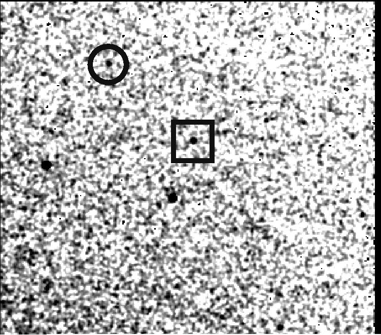
64 Figure 3.4: SuperCOSMOS and 2MASS images show UCDc-1 (2MASSJ ; squares) and WDc-1 (2MASSJ ; circles). 64

65 F5V star was observed at a similar airmass to the target to provide a telluric correction. The observing conditions were reasonable with an average seeing of arcsec. Standard iraf routines were used to reduce the spectra including flat fielding. A flatfield image was created from dome flat images by removing lamp on images from lamp off images, then median combining them using the imarith routine. This flatfield image was then normalised to 1 by creating a smoothed flatfield image, using the boxcar routine to provide the average flux in a box 11 pixels on each side. This was then divided out of the flatfield image to create a normalised masterflat. Each of the A and B images of the object, standard star and arcs were divided by the masterflat image. Cosmic rays and bad pixels were removed using an IDL program to identify bad pixels or groups of bad pixels and replace them with an average value in a 10 pixel box surrounding the bad pixel location. A-B pairs, containing a positive and negative object spectrum were extracted with apall using a chebyshev function to fit the background and a third order Legendre function (where points of deviation were removed) to trace the fit to the spectrum. The wavelength calibration was done with a Xenon arc lamp spectrum, using identify to reference the wavelength of the arc lines (from the line lists provided by the AAO; and the dispcor routine was used to correct the dispersion of the spectrum. This method was repeated for each of the differenced A-B pairs, and the wavelength calibrated spectra were median combined and flux calibrated by dividing the object spectrum by the telluric standard, then multiplying by the spectra of a blackbody, created from the bbody routine in the starlink package figaro for a T eff = 6530K (appropriate for a F5V star; see Allen s astrophysical quantities). The annotated spectra are shown in Fig. 3.5 and Fig Spectral ratios An estimate of the spectral type for 2MASSJ was based on spectral ratios used in previously published work. The J- band spectral coverage is µm. In this range the FeH ratio from Slesnick, Hillenbrand & Carpenter (2004) and the J- FeH and H 2 O A ratio from McLean et al. (2003) were used. A ratio of for FeH was measured, where FeH is the ratio of the median flux at 1.20 and 1.23µm using a bandwidth of 0.01µm (1.20/1.23µm; bandwidth=0.01µm). Using the spectral type relation from Slesnick, Hillenbrand & Carpenter (2004), a spectral type of M9 was estimated from this ratio. The J- FeH (1.20/1.185µm; bandwidth = 0.04µm) ratio of 0.85 combined with the spectral type relations from fig. 12 of McLean et al. (2003) gives a spectral range M8-L3. At 65

66 Figure 3.5: J- band spectra of 2MASSJ (thin grey line), shown with comparison spectra (thick line) of an M7, M9 and L1 type (top to bottom) from Cushing et al. (2005) overlaid. Also shown are the spectral ratios (J-FeH, FeH and H 2 O A ) used for spectral typing and the features (NaI, KI and AlI) are shown. Figure 3.6: H- band spectra of 2MASSJ (thin grey line), shown with comparison spectra (thick line) of an M7, M9 and L1 type (top to bottom) from Cushing et al. (2005) overlaid. Also shown are the spectral ratios (FeH, H 2 O B and H 2 O C ) used for spectral typing and the main KI feature. 66

67 the edge of the spectral coverage in the J- band, when strong water vapour absorption starts to appear, is the H 2 O A ratio (1.343/1.313; bandwidth = 0.004µm). This ratio was measured as The relation between H 2 O A and spectral type in fig. 11 of McLean et al. (2003) indicates an L1 type from this ratio. The H- band spectrum covers wavelengths µm, for which the H 2 O ratios from Reid et al. (2001a)[H 2 O C ] and McLean et al. (2003)[H 2 O B ] were used. The H 2 O C ratio at 1.788/1.722µm with a bandwidth of 0.004µm was measured as and indicates an L1.5 ±2 type. The H 2 O B ratio (1.48/1.60µm; bandwidth=0.02µm) of 0.9 is consistent with an M8-M9 type. All of the spectral ratios considered are indicated by dotted lines in Fig. 3.5 and Fig. 3.6 and the spectral ratio results are summarised in Table 3.2. Comparison to template spectra Template spectra of known late M and early L dwarfs were used to make a comparison to the overall profile of 2MASSJ , as well as a comparison to the absorption in spectral features such as the KI (1.168, and 1.243, µm), NaI (1.138, µm), AlI (1.311, µm) doublets in the J- band and the blended KI doublet (1.517 µm) and FeH (1.58, 1.59 and 1.62 µm) in the H- band. In general alkali metal lines weaken at the M/L boundary (McLean et al. 2000), but the NaI, AlI, FeH and KI doublets are still clearly recognisable for the purposes of a comparison. The spectra of an M7(VB8), M9(LHS2924) and L1(2MASSJ ) from Cushing, Rayner & Vacca (2005) were rebinned to the dispersion of the NIR spectra and normalised at 1.26 and 1.64 µm in the J- and H- bands respectively (Fig. 3.5 and 3.6). Visual inspection of the blended line features reveal the spectra are most consistent with an M9 type. Equivalent widths Equivalent widths for the four neutral alkali (KI) lines present in the J- band spectra were calculated using the methods of McLean et al. (2003). An IDL program was used to interactively determine the equivalent width of each KI line, which were compared with those of McLean et al. (2003) to estimate a spectral type from each line (see their table 7). In order to reduce the amount of bias when selecting the reference continuum, the process was repeated 12 times using a continuum measured at different relative positions (within 0.05 Å from the centre of the line) and a mean of the measurements taken. A 67

68 Table 3.2: Estimated spectral types for 2MASSJ Method Reference Spectral type Ratio FeH (1.200/1.230 µm) Slesnick ( 04) M9 J- FeH (1.185/1.200 µm) McLean ( 03) M8-L3 H 2 O A (1.313/1.343 µm) L1 H 2 O C (1.722/1.788 µm) Reid ( 01) L1.5 ±2 H 2 O B (1.480/1.600 µm) M8-M9 SC J-... M9 ±1 SC H-... M9 ±1 EW KI (@ µm) McLean ( 03) M8-M9 EW KI (@ µm) M7-M8 EW KI (@ µm) M7-M8 EW KI (@ µm) M7-M8 Notes: SC- Spectral Comparison, EW- Equivalent Width. width of 4.89 Å at the µm line indicates an M8/9; while the other three KI line widths at 1.177, and µm are all consistent with an M7/8 type. Analysis of the spectra of 2MASSJ , through the use of spectral ratios, comparison to template spectra and equivalent widths are summarised in Table 3.2, and are consistent with a spectral type M9 ±1. The relation between spectral type and absolute magnitude from Dahn et al. (2002) was used to calculate a range in M J of for the spectral range M8-L0. Thus, combining this with the measured J- band magnitude from 2MASS, it is estimated that 2MASSJ is at a distance of pc Spectral classification of WDc-1: 2MASSJ A spectrum of WDc-1 (2MASSJ ) was obtained with FORS1 on the VLT on 2007 January 24, with Directors Discretionary Time in programme 278.C-5024(A), using the longslit mode in the optical wavelength range Å and a dispersion of 50 Å/mm. Three integrations of 600s were taken, giving a total exposure time of 30 minutes. Spectra of a DC WD and a standard F-type star were also taken and used for calibration. Sky flats were taken and HgCd arcs were used for wavelength calibration. 68

69 Figure 3.7: Optical spectrum of the confirmed white dwarf WDc-1 (2MASSJ ), flux calibrated and normalised at 4600Å. Standard IRAF packages were used to reduce the spectra including debiasing (by creating a master bias frame from median combined images and subtracting this from the object, standard star, flat field and arc images), flat fielding and removal of bad pixels. The three spectra were then extracted and wavelength calibrated as described in The resulting spectra of both WDc-1 and the standard were divided by the featureless DC WD spectrum, which has no intrinsic spectral features, enabling correction for the instrumental response. The standard star was then used for flux calibration and the final spectrum of 2MASSJ is shown in Fig WD parameters, T eff and log g were derived from a fit of the Balmer lines using the fitting routine fitprof described in Napiwotzki, Green & Saffer (1999). The WD spectrum was modelled using an extensive grid of spectra computed with the model atmosphere code of Detlev Koester described in Finley, Koester & Basri (1997). Observational and theoretical Balmer line profiles were normalised to a linear continuum and the atmospheric parameters determined with a χ 2 algorithm. The best fit is shown in Fig The results are T eff = 7600 ± 20 K and log g = 8.09 ±0.04 (formal uncertainties from the fit routine to one sigma). 69

70 Table 3.3: Fit results and derived quantities for WD mass, cooling age and absolute magnitude for the corrected and uncorrected case discussed in T eff log (g) M t cool M V K dex M Gyr solution solution Realistic uncertainty estimates are often substantially larger than the formal statistical estimates. Napiwotzki et al. (1999) derived a relative uncertainty of 2.3% in T eff and dex in log g from a sample of DA WDs analysed using the same fitting method. This temperature uncertainty was adopted for the following estimates, but the gravity determination is likely subject to a systematic overestimate. The mass distribution of WDs peaks close to 0.6 M (e.g. Napiwotzki, Green & Saffer 1999; Bergeron, Gianninas & Boudreault 2007), corresponding to log g values close to 8.0. Spectroscopic investigations applying the method have shown a trend of the log g distribution peaking at increasingly higher values for decreasing temperatures (Bergeron, Gianninas & Boudreault 2007). This trend starts at 11,500 K putting the WD analysed here in the affected region. Taken at face value, this would indicate on average higher masses for cool WDs. However, as argued by Bergeron, Gianninas & Boudreault (2007) and Engelbrecht & Koester (2007) this can be ruled out. A source of extra line broadening must be present in these stars. However, the exact nature of this mechanism is still under discussion and as pointed out in Bergeron, Gianninas & Boudreault (2007) anecdotal evidence suggests that some stars are affected and others are not. A pragmatic approach was taken here, where a large sample of DA white dwarfs were used from observations taken in the course of the SPY programme (Napiwotzki et al. 2001) to derive an empirical correction. Spectra of these stars have been previously analysed using the same model grid and very similar analysis methods as for the WD discussed here. The estimated shift in log g distribution caused by the unknown mechanisms is 0.3 dex in the T eff = K range. The corrected gravity is thus log g=7.79. As mentioned above it is not entirely clear whether all cool WDs are affected. Thus the corrected and uncorrected gravity values will be used for further discussion. WD masses and cooling ages were calculated by interpolation in the Benvenuto & Althaus (1999) cooling tracks for WDs with thick hydrogen envelopes. Results are listed in Table

71 Figure 3.8: Model atmosphere fit to the Balmer lines of 2MASSJ giving best fit parameters of T eff = 7600 K and log g=7.79. Observed and theoretical fluxes were normalised to the continuum. Line profiles are shifted for clarity. 71

72 3.3.3 A randomly aligned pair? In order to determine if the new system is a bonafide UCD + WD binary, the likelihood that two such objects could be a line-of-sight association with photometry and proper motion consistent with binarity by random chance has been statistically assessed. To do this, firstly the UCD luminosity function of Cruz et al. (2007) was taken, which gives a number density of (4.9 ±0.6) 10 3 UCDs per pc 3 for M7-M9.5 types. Then a volume associated with 1532 circular areas on the sky (one for each of the WD candidate sample), with radii of 89 arcsec (separation of the components) and a line-of-sight depth of 58 ±17pc (approximate distance to the new M9 UCD, using relations from Dahn et al. 2002) were calculated. This volume equates to 58 ±26 pc 3, giving a total expected number of 0.28 UCDs to be within 89 arcsec of one of the WD candidates. To factor in the probability that two objects might have a common proper motion at the same level as the measurements, a magnitude-limited sample (R <20) was downloaded from the SuperCOSMOS Science Archive (SSA), applying the same minimum proper motion requirement that was used to create the WD candidate sample. A magnitude limited sample of 160 sources, selected from a large circular sky radius of 90 arcmin centred on the WD. A proper motion vector-point-diagram was constructed and sources counted that were found to be within the 2 σ uncertainty circle of the measured UCD proper motion. Four of the 160 sources had proper motion consistent with the UCD, suggesting a probability of 2.4 ±1.2% that such common proper motion could occur by random chance (where Poisson uncertainties associated with this and other samples were considered here). An additional requirement fulfilled by the UCD + WD system is that the colourmagnitude information must be consistent with a common distance (see Fig. 3.3) and 53% (786 ± 28) of the WD candidate sample were found to be photometrically consistent with being at the same distance as the UCD. Finally considered was the fraction of WD candidates that might be spurious and thus not able to contribute to non binary line-of-sight associations where the WD has been confirmed spectroscopically. In the magnitude range R < 14, where MS99 is thought to be essentially complete, it was find that 66% of our WD candidates are included in the MS99 catalogue. This suggests that, at least for brighter magnitudes, the WD candidates presented here are relatively free from contaminating objects, and that the selection techniques are robust. While it cannot be guaranteed that the same low-level of 72

73 contamination applies to the full magnitude range, a conservative approach was taken, by assuming that the full WD candidate sample could potentially contribute to non-binaries that appear to be UCD + WD pairs. Taking into account all these factors, it is estimated that one would expect ± randomly aligned UCD + WD pairs with 89 arcsec separation, proper motion and photometry consistent with binarity at the level of the observations. The likelihood of the system being merely a line-of-sight association is thus vanishingly small, and it can thus be assumed that the UCD + WD pair is a gravitationally bound binary system Binary age The age of the binary system can be constrained from the WD mass and cooling age. For the corrected fit, 2MASSJ has a mass of 0.48 M and a cooling age of 0.94 Gyr. The IFMR determinations of Weidemann (2000), Dobbie et al. (2004), Dobbie et al. (2006), Ferrario et al. (2005), Catalán et al. (2008) and Kalirai et al. (2008) were assessed to estimate a likely, initial-mass constraint for the main-sequence progenitor star of 1 2 M. The main-sequence lifetime of a progenitor of this mass is likely >1 Gyr (probably several Gyr) and thus is not useful when trying to constrain the upper age limit of the system. Note that if the WD mass were higher, for example if the helium enrichment of the atmosphere is lower than typical (see 3.3.2) then the WD s log g could be as high as 8.1 dex, with a WD mass of 0.65 M and cooling age of 1.5 Gyr. This would allow the progenitor mass to be constrained to a likely range of > 2.7 M, giving a main-sequence progenitor lifetime of < 0.83 Gyr (Monteiro et al. 2006) and a binary age constraint of Gyr. This possibility is instructive at least in demonstrating the level of age constraints (with accompanying UCD constraints) that may be placed on benchmark binaries of this type. However, it is not possible to judge the helium content of the WDs atmosphere (if any) and thus only a lower limit can be confidently placed on the age of this binary from the best fit cooling age for the WD, combined with an estimate of the main-sequence lifetime of the progenitor, which is likely equal to or larger than the WD cooling age. The age of the binary is thus > 1.94 Gyr. 73

74 3.3.5 UCD properties T eff, mass and log g have been estimated from the Lyon group DUSTY models (Chabrier et al. 2000c; Baraffe et al. 2002), using the minimum age of the system (1.94 Gyr) and an estimated M J for 2MASSJ The models indicate that 2MASSJ has T eff = K, mass= M and log g= , placing it close to the limit for hydrogen burning. Note that the estimated T eff is consistent with the semi-empirical estimates of Golimowski et al. (2004) for an M9 ±1 dwarf, which use well measured luminosities and a model constraint on radius (which changes by <10% for ages of 1 5 Gyr) to determine T eff values spanning a wide range of spectral type. The full list of properties for the binary are listed in Table Searching SDSS and UKIDSS A search for widely separated binary systems from a selected sample of WDs and UCDs from SDSS and UKIDSS (as described in and 2.2.2) was conducted using a similar method as was used for the 2MASS and SuperCOSMOS search (described in in 3.2) Simulated numbers of WD + UCD binaries The number of potential WD + UCD binary systems that could be detected in the full coverage of SDSS and UKIDSS was estimated by Pinfield et al. (2006), who suggest that benchmark systems (with ages known to 10%) could be found out to a limiting magnitude of J The number of non-benchmark systems (where the WD <0.7M ) that could also be identified is estimated at five times that number, suggesting that up to 300 WD + UCD systems could be identified by combining UKIDSS with SDSS. Corresponding photometric properties were also derived and are shown in Fig The level of contamination from other objects such as high velocity stars (e.g. halo objects or red giants) was estimated at 400, which is comparable to the number of real systems expected via photometric selection alone. However, measuring a common proper motion for the components of potential systems should remove the majority of the contamination. 74

75 Table 3.4: Parameters of the binary 2MASSJ MASSJ and its components. Parameter Value Separation on sky arcsec Estimated distance pc Estimated line-of-sight separation AU Minimum age of system... > 1.94 Gyr Ultracool Dwarf RA DEC MASS designation... 2MASSJ Distance pc 2MASS J ± MASS H ± MASS K s ± 0.06 DENIS I ± 0.23 DENIS J ± 0.14 SuperCOSMOS I µ RA ±30 mas yr 1 µ DEC ±20 mas yr 1 Spectral Type... M9 ±1 Mass M T eff K log g dex White Dwarf RA DEC MASS designation... 2MASSJ Distance pc 2MASS J ± MASS H ± 0.15 DENIS I ± 0.07 DENIS J ± 0.22 SuperCOSMOS B SuperCOSMOS R SuperCOSMOS I µ RA ±30 mas yr 1 µ DEC ±12 mas yr 1 Spectral Type... DA T eff ±175 K log g dex Mass M WD cooling age Gyr WD progenitor age... > 1 Gyr 75

76 Figure 3.9: Simulated WD + UCD J- against g- magnitude diagram from Pinfield et al. (2006), showing a simulated population of WD + UCD binaries (dots) covering 10% of the sky for J Potential benchmark systems (WD 0.7M ) are shown as plus symbols Binary selection To select binary system candidates, firstly distance constraints were placed on the sample of WD candidates selected from SDSS using a CMD for WDs with known parallax from McCook & Sion (1999) in the SDSS colour system as shown in Fig In the same way as described in 3.2, this was used to estimate a lower distance for the WD candidate and thus a maximum separation based on a mass of 1.2M. UCD candidates were searched for out to an angular separation from each WD candidate corresponding to a projected separation of 20,000AU at this estimated distance. In order for a good UCD companion to be selected it must have a distance consistent with the WD it is paired with. This was assessed by placing the candidate UCD companion on a M J against J H CMD, where M J was calculated from the WD lower distance estimate and the UKIDSS J- band magnitude. The J H colour was chosen here, instead of the previously used J K colour (for L dwarf candidates in 2MASS), as T dwarfs have bluer NIR colour and can thus be very faint in the K- band. Selection regions were defined using known L and T dwarfs with measured parallax from dwarfarchives.org. The regions defining these areas are shown as dotted (L) and dashed (T) line boxes, as illustrated in Fig and 76

77 Figure 3.10: A WD colour-magnitude diagram for MS99 WDs with known parallax (crosses with error bars). Photometry is on the SDSS system. Overplotted are model cooling tracks (see 3.4.1) for WD masses of 0.5, 0.7 and 1.2 M (dotted, dashed and dot-dashed lines respectively). The selected WD region in the CMD lies between the two solid lines. were chosen to select objects with the most compelling UCD colours whilst minimising contamination from main-sequence stars. It is also noted that there is some cross over in the position of some late L and early T dwarfs, as is also shown by Knapp et al. (2004). The selection used here is flexible enough to account for this by allowing objects that have L dwarf Y J and J H colours, that also pass the T dwarf M J, J H CMD criteria to be selected as possible L/T transition objects. Candidate early/mid L dwarfs were selected if they occupy the L box in two-colour space (Fig. 2.5) and the corresponding L box in colour-magnitude space (Fig. 3.11). If an object is found in the L box in two-colour space and the T box in colour-magnitude space then is it selected as an L/T transition object, likewise a candidate T dwarf is selected if its position lies in the T box in both colour and colour-magnitude selections. The criteria for the three selections are outlined here: 77

78 Figure 3.11: A UCD colour-magnitude diagram for L (plus symbols) and T (diamonds) dwarfs with known parallax from dwarfarchives.org. The selection regions for L and T dwarfs are overplotted as dotted and dashed lines, respectively. Early/Mid L dwarf colour and magnitude selection criteria: 0.4 < J H < 1.2, 0.9 < Y J < 1.5 and 11.0 < M J < 15.0, M J < 8.5(J H) criteria: Late L/Early T dwarf (i.e. L/T transition objects) colour and magnitude selection 0.4 < J H < 1.2, 0.9 < Y J < 1.5 and 13.5 < M J < 17.0, M J > 8.5(J H) Mid/Late T dwarf colour and magnitude selection criteria: 0.5 < J H < 0.4, 0.9 < Y J < 1.25 and 13.5 < M J < 17.0, M J > 8.5(J H)

79 An IDL program was written to search for candidate pairs amongst the 22,087 WD and 24,293 UCD candidate objects using these selection criteria, which resulted in a sample of 517 candidate binary systems Candidate WD + UCD systems As SDSS covers a large section of sky common to that of UKIDSS, the UCD candidates were cross matched with objects in the SDSS DR6 database, using the cross matching facility in a 2 arcsec radial search, which should detect any optical component for objects with a proper motion of less than 1 arcsec/yr. The UCD candidate sample was then split up into two categories; optical and non-optical detections. Properly assessing the optical non detections would require further follow-up beyond the scope of this thesis. For the optical detections additional colour cuts were used, based on the objects optical and optical-nir colours. Hawley et al. (2002) show that L and T dwarfs are separated quite well using i z and z J colours and suggest that i z > 1.6 would select M8 and later type dwarfs. Indeed Fan et al. (2001) and Chiu et al. (2006) select L and T dwarfs where i z > 2.2 and z J > 2.0. An i r colour could also be used, however many UCDs are very faint in the r- band and photometry can be unreliable. Following this approach, good L and T dwarf candidates were selected if they had i and z band SDSS counterparts with 5σ detections (corresponding to the approximate SDSS 5σ limits; i < 21.3 and z < 20.8), i z > 1.75, and z J > 2.0. Additionally a subset with 1.6 < i z < 1.75 and z J > 2.0 were also selected as candidate UCDs. Non i band detections or drop outs were also considered, where the z J colour limits are consistent with being UCD like. By including this optical selection the candidate list was reduced from 517 to have no optical counterpart within 2 arcsec of their NIR coordinates (implying i > 21.3 and z > 20.8) and are shown in Tables 3.11 and 3.12 as candidates named nbinx (where x is the identifying number). 18 are i band drop outs and are shown in Tables. 3.9 and 3.10 as candidates with name ibinx. 34 are good late M candidates, having 1.6 < i z < 1.75 and z J > 2.0 (Shown as candidates mbinx in Tables. 3.7 and 3.8). 36 are good L and T candidates based on their optical and optical-nir colours (i z > 1.75 and z J > 2.0) and labelled as candidates bbinx in Tables. 3.5 and 3.6. These 156 candidates were also eyeballed in the UKIDSS/WFCAM images and the SDSS optical images to remove any spurious survey detection or non-star like objects. None of the candidates showed any 79

80 Figure 3.12: Left: i z against spectral type relation. Right: z J against spectral type relation from Hawley et al. (2002), showing means colours for each spectral type and the standard deviation of the measurements as error bars. Figure 3.13: Colour-colour relations from Hawley et al. (2002). M dwarfs are shown as squares and plus signs, early L dwarfs as triangles, late Ls as crosses and Ts as diamonds. 80

81 sign of being spurious and are thus plotted in Figs and In addition the WD candidates were cross matched with the SDSS spectroscopic catalogue to check if any had spectra that could confirm them, or not as such. Of the 156 candidate WDs, 71 had spectra available from SDSS. Of these 36 are flagged as being WD (DA) targets and 35 are flagged as being star like. This classification may not just contain main-sequence stars or late-type stars, but may include more unusual WD types (DB, DC, DO, DQ, DZ) as well as unresolved, spectroscopic binaries containing a WD member. Proper motion measurements were also checked for in the SDSS archive, which are measured by matching SDSS positions against the USNO-B1.0 catalogue (Monet et al. 2003). Details of all 156 candidate binary pairs are shown in Tables Second epoch imaging and proper motion analysis of candidate UCDs One of the candidate binary systems (bbin1) has spectroscopically confirmed components as a DA WD and an L3 dwarf, however on inspection of the published proper motion of the WD (from SDSS) and the L dwarf (Jameson et al. 2008) they do not appear to share a common proper motion and this pair were thus ruled out as a potential binary system. Additional pairs were prioritised from the list of candidates (where the WD component had a measured proper motion of >100mas/yr) for follow-up second epoch imaging on IRIS2/AAT during February. Nine candidates were imaged in the J-, H- and K- bands during poor weather time (seeing > 2 arcsec). The images were reduced using the oracdr package for IRIS2 and proper motions calculated using the iraf routines geomap and geoxytran using an average of 15 reference stars, as is described in In the majority of cases the motion was less than a pixel and the baseline on average only 1 yr. Combined with high residuals of the transformations from the WFCAM/UKIDSS images onto the IRIS2/AAT images resulted in high uncertainties in the measurements. The proper motions of the nine UCD candidates, along with the measured proper motion of the WD counterpart are shown in Table Uncertainties were calculated from the residuals of the transformation combined with centroiding uncertainties of ±0.5 pixels. Of the nine candidates measured two were deemed to be non-common proper motion and seven remain uncertain. In order to confirm the binary nature of these remaining seven candidate systems an additional epoch image is needed, ideally with a longer baseline. Candidates bbin17, bbin26 and bbin29 appear to have a sizeable proper motion, 81

82 Figure 3.14: Left: A Y J against J H two-colour diagram. Right: An M J against J H CMD of UCD candidate components of potential wide WD + UCD binaries. Blue plus symbols show L and T dwarf candidates with good optical colours, red asterisks are i band drop outs, red diamonds are non-optical detections and black triangles are UCD candidates with good optical colours, also overplotted are main-sequence stars as green dots. The open square shows the widely separated UCD candidate system from the spectroscopic WD + M dwarf (nbin7; see 3.4.4). Also shown are the L and T dwarf selection regions (dotted and dashed boxes, respectively). 82

83 Figure 3.15: A u g against g r two colour diagram showing WD candidate components of potential wide WD + UCD binaries. Blue plus symbols show WD candidates whose L and T dwarf candidate counterparts have good quality optical colours, red asterisks are i band drop outs and red diamonds are optical non-detections, also overplotted are spectroscopically confirmed WDs as green crosses. The open square shows the widely separated WD candidate that appears to be an unresolved WD + M dwarf binary system (nbin7; see 3.4.4). 83

84 Table 3.5: Parameters of the WD component of the WD + UCD binary candidates, where L and T dwarf candidates have optical colours i z >1.75 and z J >2.0. ID WD RA WD DEC g u g g r M g D MIN SDSS a WD? b PM c pc spectra? mas/yr bbin y y 8.0 bbin n bbin y? 53.0 bbin y y 13.3 bbin y y 2.2 bbin y? 2.4 bbin n bbin n bbin n bbin n bbin n bbin n bbin n bbin y y 5.1 bbin n bbin n bbin y? bbin y? 20.6 bbin n bbin n bbin y y 4.8 bbin y y bbin n bbin n bbin y y 29.0 bbin y? bbin n bbin n bbin y y bbin n bbin n - n bbin y y 5.4 bbin n bbin y? n bbin n bbin n - n Notes: a A spectrum is available from SDSS. b SDSS target as WD or is classified as a WD.? - SDSS classification is star but may be a more unusual type of WD (i.e. DB, DC, DO, DQ, DZ). c proper motion as measured by SDSS. 84

85 Table 3.6: Parameters of the UCD component of the WD + UCD binary candidates, where L and T dwarf candidates have optical colours i z >1.75 and z J >2.0. ID UCD RA UCD DEC J J H Y J M J Separation Separation i z z J degs degs arcsec AU bbin bbin bbin bbin bbin bbin bbin bbin bbin bbin bbin bbin bbin bbin bbin bbin bbin bbin bbin bbin bbin bbin bbin bbin bbin bbin bbin bbin bbin bbin bbin bbin bbin bbin bbin bbin

86 Table 3.7: Parameters of the WD component of the WD + late M dwarf binary candidates selected from SDSS and UKIDSS. ID WD RA WD DEC g u g g r M g D MIN SDSS a WD? b PM c pc spectra? mas/yr mbin y y 2.7 mbin y? 9.0 mbin y? 76.0 mbin y y 1.7 mbin y y 6.8 mbin y? 4.7 mbin y y 1.1 mbin y y 16.0 mbin y y 1.1 mbin y y 6.8 mbin n mbin n mbin n - n mbin y? 11.6 mbin n mbin y y 63.0 mbin y y 4.0 mbin n mbin n mbin n mbin y y 1.4 mbin n mbin y? 0.6 mbin y y 1.9 mbin n mbin n mbin n mbin n - n mbin n mbin n mbin n mbin y y mbin y y mbin n Notes: a A spectrum is available from SDSS. b SDSS target as WD or is classified as a WD.? - SDSS classification is star but may be a more unusual type of WD (i.e. DB, DC, DO, DQ, DZ). c proper motion as measured by SDSS. 86

87 Table 3.8: Parameters of the UCD component of the WD + late M dwarf binary candidates selected from SDSS and UKIDSS. ID UCD RA UCD DEC J J H Y J M J Separation Separation i z z J degs degs arcsec AU mbin mbin mbin mbin mbin mbin mbin mbin mbin mbin mbin mbin mbin mbin mbin mbin mbin mbin mbin mbin mbin mbin mbin mbin mbin mbin mbin mbin mbin mbin mbin mbin mbin mbin

88 Table 3.9: Parameters of the WD component of the WD + UCD i- band drop out binary candidates selected from SDSS and UKIDSS. ID WD RA WD DEC g u g g r M g D MIN SDSS a WD? b PM c pc spectra? mas/yr ibin n ibin y? 4.5 ibin n ibin n ibin y? 27.0 ibin y y 4.8 ibin y y 6.0 ibin n ibin y? n ibin n ibin y y 7.6 ibin n ibin n - n ibin y? n ibin n - n ibin n - n ibin n - n ibin n - n Notes: a A spectrum is available from SDSS. b SDSS target as WD or is classified as a WD.? - SDSS classification is star but may be a more unusual type of WD (i.e. DB, DC, DO, DQ, DZ). c proper motion as measured by SDSS. 88

89 Table 3.10: Parameters of the UCD component of the WD + UCD i- band drop out binary candidates selected from SDSS and UKIDSS. ID UCD RA UCD DEC J J H Y J M J Separation Separation z J degs degs arcsec AU ibin ibin ibin ibin ibin ibin ibin ibin ibin ibin ibin ibin ibin ibin ibin ibin ibin ibin

90 Table 3.11: Parameters of the WD component of the WD + UCD non-optical detection binary candidates selected from SDSS and UKIDSS. ID WD RA WD DEC g u g g r M g D MIN SDSS a WD? b PM c pc spectra? mas/yr nbin y? 2.9 nbin n nbin y y 29.0 nbin y y 15.0 nbin y y 55.9 nbin y y 5.2 nbin y? nbin y? 7.0 nbin y? 13.0 nbin y? 12.5 nbin y? 2.2 nbin y y 19.6 nbin n nbin y y nbin n - n nbin y y 92.9 nbin y? 26.6 nbin n nbin n - n nbin n nbin y? 24.8 nbin n nbin n nbin y? 2.7 nbin y? n nbin y? 2.8 nbin y? 5.7 nbin y? 3.5 nbin y? 3.5 nbin y? 11.6 nbin n nbin n

91 nbin y y n nbin y? 35.0 nbin y? n nbin y? 35.0 nbin n nbin n nbin y y 1.7 nbin y? 5.1 nbin y y 4.7 nbin y y 46.7 nbin y? 60.6 nbin n - n nbin n - n nbin n - n nbin n - n nbin n - n nbin n - n nbin n - n nbin n - n nbin n - n nbin n - n nbin n - n nbin n - n nbin n - n nbin n - n nbin n - n nbin n - n nbin n - n nbin n - n nbin n - n nbin n - n nbin n - n nbin n - n nbin n - n nbin n - n nbin y - n Notes: a A spectrum is available from SDSS. b SDSS target as WD or is classified as a WD.? - SDSS classification is star but may be a more unusual type of WD (i.e. DB, DC, DO, DQ, DZ). c proper motion as measured by SDSS. 91

92 Table 3.12: Parameters of the UCD component of the WD + UCD non-optical detection binary candidates selected from SDSS and UKIDSS. ID UCD RA UCD DEC J J H Y J M J Separation Separation degs degs arcsec AU nbin nbin nbin nbin nbin nbin nbin nbin nbin nbin nbin nbin nbin nbin nbin nbin nbin nbin nbin nbin nbin nbin nbin nbin nbin nbin nbin nbin nbin nbin nbin nbin

93 nbin nbin nbin nbin nbin nbin nbin nbin nbin nbin nbin nbin nbin nbin nbin nbin nbin nbin nbin nbin nbin nbin nbin nbin nbin nbin nbin nbin nbin nbin nbin nbin nbin nbin nbin nbin

94 Table 3.13: Proper motion analysis for followed up candidate WD + UCD binary pairs from SDSS and UKIDSS Candidate PM RA PM DEC Baseline PM Pixel PM Pixel CPM? UCD (WD) (WD) RA a Motion DEC a Motion mas/yr mas/yr yr mas/yr (RA) mas/yr (DEC) bbin1 b No bbin ± ± ? mbin ± ± ? bbin ± ± No bbin ± ± ? bbin ± ± ? bbin ± ± No mbin ± ± ? nbin ± ± ? nbin ± ± ? Notes -? Indicates uncertainty, due to high uncertainties and small measured motions a - uncertainties on the proper motion from fit to the residuals of the transformation only. b - UCD PM measurement from Jameson et al. (2008). typically at least 100mas/yr if being conservative with the associated errors and taking them at their largest values. This would indicate that these objects, despite two of them being non-common proper motion with their paired WD may still be UCDs, as their sizable motion is indicative of a close by object. There may however still be some contamination from high proper motion halo objects. Spectroscopic follow-up would be required to confirm these as UCDs A candidate wide L dwarf companion to a spectroscopic WD + M dwarf binary Of the nine candidates that were followed-up seven had spectra in SDSS, five of which were flagged as WDs, one flagged as being unknown and one has a spectra that appears to show that it is an unresolved WD + M dwarf binary. This candidate is the counterpart to the UCD candidate nbin7 (from Tables and 3.13, which is an L dwarf candidate at a projected separation of 19,500AU). The SDSS spectrum is shown in Fig. 3.16, where 94

95 Figure 3.16: SDSS spectra of the WD candidate nbin7. the hydrogen Balmer lines of a DA WD are clearly visible at the blue end and features of a cooler M dwarf, such as the VO feature at 7500Å, NaI at 8200Å and CaH at 7050Å can be seen at the red end of the spectrum. Estimating spectral types of the WD and M dwarf In order to establish the WD and M dwarf contribution to the spectra, convolved spectral models were constructed. Template WD spectra were taken from the SDSS DR1 WD spectroscopic catalogue of Kleinman et al. (2004) and template M dwarf spectra were taken from Bochanski et al. (2007), who have co-added many spectra of the same spectral type to create template spectra for M0-L0 covering the SDSS wavelength range ( Å). The WD and M dwarf spectra were both rebinned to the same dispersion and wavelength range as the original SDSS spectra. The WD and M dwarf components were then individually scaled to the peak of the flux of the WD and M dwarf, respectively. The WD was firstly normalised to the flux peak in the SDSS reference spectrum at 4000Å the M dwarf spectrum was then scaled to the peak of the flux of the M dwarf component at 8080Å in the SDSS reference spectrum. Both components were then smoothed to the same resolution as the SDSS reference spectra and finally combined together, by adding the WD and M dwarf components. This was repeated for different combinations of DA WD and UCD (M0-L0) and overplotted onto the original SDSS spectra for visual comparison. 95

96 The best fit to the SDSS spectra was found by visually inspecting the fit to the model spectra. On first inspection the best fit to the WD comes from a DA4/5. The WD + M dwarf spectra for a DA4 and DA5 are shown in Figs and On closer inspection to the depth and width of the Balmer lines and the depth of the features in the M dwarf combined with the overall fit, the best fitting spectral combination is provided by a DA4 + M4, as shown in Fig To verify the spectral type of the M dwarf and check for any possible spectroscopic peculiarities, the model DA4 was deducted from the original SDSS spectrum and spectral ratios covering the wavelength range Å were assessed, including the pseudocontinuum (PC) ratios from Martín, Rebolo & Zapatero-Osorio (1996) and Martín et al. (1999). The PC ratios use points in the spectrum that are less affected by molecular opacity that cause the true stellar continuum to be suppressed, causing a pseudocontinuum. The PC1, PC2 and PC3 ratios were used over this wavelength range ( Å). The PC1 ratio (the mean flux in the ranges Å/ Å) gave a ratio of 1.406, which corresponds to a spectral type of an M4/5 from table 3 of Martín, Rebolo & Zapatero-Osorio (1996). The PC2 ratio ( Å/ Å) was measured as 1.677, indicating an M5 type. The PC3 ratio was also assessed, which is used as the primary index for spectral typing by Martín et al. (1999). The ratio ( Å/ Å) was measured as 1.148; indicating an M4 type. This verifies the M4 type that was initially estimated from the model comparison with the convolved spectra. The M4 spectra with the DA4 model removed is shown in Fig. 3.20, with the model M4 spectra overplotted for comparison. An age estimate for the WD + M4 system The spectrum of the M4 (with the WD component removed) can also be used to place a crude age estimate on the age of the system. West et al. (2008) calculated an age-activity relation for M dwarfs based on their Hα emission. Activity in M dwarfs has been shown to decrease over time and suggests that it is thus limited to a finite age (Fleming, Schmitt & Giampapa 1995; Gizis, Reid & Hawley 2002). If stars are still active they should show prominent Hα emission at 6562Å. The M dwarf spectra here (shown in Fig. 3.20), was compared to the template spectra of active and non-active M dwarfs from Bochanski et al. (2007) and shows no evidence of Hα emission. West et al. (2008) calculate an activity lifetime of Gyr for an M4 dwarf, which suggests that this system is 3.5 Gyr. 96

97 Figure 3.17: Model DA4 WD spectra combined with M0-L0 (top to bottom) spectra (solid lines) overplotted with the original SDSS spectra (red dotted lines) over the wavelength range ( Å). 97

98 Figure 3.18: Model DA5 WD spectra combined with M0-L0 (top to bottom) spectra (solid lines) overplotted with the original SDSS spectra (red dotted line) over the wavelength range ( Å). 98

99 Figure 3.19: Model DA4 WD combined with an M4 spectra (solid line), overplotted with the original SDSS spectra (red dotted line) over the wavelength range ( Å). Figure 3.20: M4 component of the convolved spectra (solid line), created from the original SDSS spectra - model DA4 spectra, overplotted with the M4 model spectra (red dotted line). 99

100 Thus if the UCD wide binary candidate is confirmed as so, through proper motion and spectral analysis, it will have at least an independent minimum age constraint. 3.5 Summary of chapter This chapter has presented the search for UCD companions to WDs using archival data from SuperCOSMOS and 2MASS, including the discovery of the widest separated UCD + WD binary system. Also presented were a large number of candidate UCD + WD systems from SDSS (DR6) and UKIDSS (DR3). Of these 156 candidate binaries, 10 UCD components have been followed-up with second epoch imaging to assess their proper motion. Three were found to be non-common and thus not UCD + WD binary systems. The other seven remain uncertain due to high uncertainties associated with their measurements arising from a combination of a short baseline and a small motion of the object. One of these uncertain systems however has a spectroscopic WD + M4 primary, which has a minimum age constraint of 3.5 Gyr, based on the non-presence of Hα in the M dwarf spectrum and the age-activity relations from West et al. (2008). Thus if this UCD is confirmed as such it will be add to the complement of UCDs with known ages and be able to provide useful information for trends in properties with age. Further studies of the WD will also allow an additional verification of the age of the system. Indeed if the WD proves to have a high mass, it is likely to yield an age constraint to within 10% accuracy, which would make it an ideal benchmark system. The other candidates, along with the four systems (UCD5, 6, 7 & 8) remain uncertain from the search of SuperCOSMOS and 2MASS. All require additional epoch imaging to properly assess if their motion is common to their paired WD. Subsequent spectroscopy of any confirmed common proper motion systems would also be needed to confirm their nature as UCDs. The sample however looks promising for potentially finding a large number of UCD companions to WDs at wide separations. If confirmed these will greatly increase the number of such systems known as well as providing useful age constraints. 100

101 Chapter 4 Ultracool companions to Subgiants Presented in this chapter is a search for widely separated UCD companions to subgiant stars in the southern hemisphere through a NIR imaging survey. The observational strategy, calibration and analysis is described that allows the selection of good candidate binary systems. In addition, the followup methods, subsequent analysis and the findings so far are summarised in the following sections. 4.1 A pilot survey of southern Hipparcos subgiants A pilot survey was carried out to search for UCD companions to Hipparcos subgiants via NIR imaging, using the 3.9m Anglo-Australian Telescope (AAT) and the IRIS2 instrument (in wide field imaging mode) over an eight night run in 2005 December. The FOV allows for wide separations to be probed with relatively short integration times, enabling a subgiant to be efficiently imaged in three NIR filters over approximately 20 minutes per target Selection of subgiants The subgiant sample were selected from the Hipparcos catalogue (Perryman et al. 1997) and as described in Pinfield et al. (2006), a publication on which I collaborated. Selected subgiants have well measured magnitudes, parallax distances and a large number have a constrained mass, age and metallicity from Feltzing, Holmberg & Hurley (2001) and from Nordstrom et al. (2004), who both derive metallicity from Strömgren photometry and then 101

102 use stellar evolution models to infer a corresponding age. Subgiants were selected based on their position on a M V against B V CMD for stars with V < 13.0 and B V > 0.6. A parallax measurement constraint was also imposed such that π/σ 4, leading to an uncertainty in the parallax of 25%. A range in M V of was also chosen to avoid the brightest subgiants, for which glare may become as issue when trying to image faint, closely separated UCD companions, whose signal may be hidden by the PSF wings of very bright subgiants, which can extend for several arcsec. The colour cuts were defined to select against dwarfs and giant stars, as shown by the selection boxes in Fig. 4.1, using solar metallicity isochrones from Girardi et al. (2000) as a guide. Note that these isochrones become bluer and brighter for lower metallicity and it is therefore possible that some contamination may arise from sub-solar metallicity giants in the top right of the selection region. To help minimise this contamination any objects spectroscopically flagged as giants in the Hipparcos database were removed from the sample. Another issue considered was interstellar reddening, that could make it difficult to separate L dwarfs photometrically from reddened background objects. Therefore subgiants in reddened regions where galactic extinction was higher than A V > 0.3(E J K < 0.05) (derived from the reddening maps of Burstein & Heiles 1982) were removed from the sample. Areas of overcrowding were also avoided as blended point source profiles may become problematic when extracting photometry. These areas included the galactic plane, LMC, SMC and some areas where the nearest neighbouring object was <10 arcsec away. Subgiants with small proper motions (< 40mas/yr) were also removed, as confirmation of UCD companions will be based partially on subsequent proper motion measurements. If a subgiant has a small proper motion it will be difficult to confirmation a UCD companion through common proper motion over a short baseline. Finally a distance constraint of 160pc was imposed, as L and T dwarfs at distances greater than this would have apparent brightnesses that are too faint to be detected in the exposure times that were used. This set of selection criteria gave a target sample of 918 subgiants Simulated populations Simulations of the expected number of UCD companions to subgiants that could be discovered with imaging observations was presented in Pinfield et al. (2006). This was based on a simulated disk population of subgiants. A Salpeter mass function was assumed, with a birth rate history from Rocha-Pinto et al. (2000) and a disc scale height-age 102

103 Figure 4.1: Subgiant selection. (a) An M V against B V diagram of Hipparcos stars with V < 13.0 and π/σ 4. (b) Theoretical isochrones from Girardi et al. (2000) for solar metallicity. Overplotted as boxed areas in both plots is the subgiant selection region. 103

104 relation from Just (2003). A metallicity distribution was taken from Edvardsson et al. (1993) and UCD companions were randomly added to the simulation around 34% of the subgiant sample (the wide binary fraction from Pinfield et al. 2006, although uncertainties associated with this fraction were also taken into account), with separations uniformally distributed between AU. An age distribution for the UCDs was derived for the subgiant sample and a UCD mass function of a power law where α=1 (following Gizis et al. 2001) was imposed. Lyon group models were used to derive T eff, log g and M J from UCD mass and age, and a J- band magnitude was calculated for the distance of the subgiants. This simulated distance-magnitude and separation-distance distribution is shown in Fig. 4.2 and 4.3, respectively. Also shown in 4.3 is the glare limit, which corresponds to the minimum separation that could be imaged around a star. This was calculated from the brightness of the object. The brighter the object the larger the PSF wings (glare), however brighter objects are also generally closer and so separations of a few arcsec, correspond to only a few AU at these distances. This effectively causes the two effects to cancel each other out, creating a nearly vertical glare limit. A photometric limit of J 20 was also imposed on the selection of simulated UCD companions, such that UCD candidates could be spectroscopically followed up on an 8m class telescope. The simulation predicts that L and T dwarfs with J 20 might be detectable around a sample of 918 subgiants within a distance of 160pc, across the whole sky. Note that this value, obtained from simulations is indicative rather than rigorously quantitative. 4.2 The pilot survey Imaging of a subset of the sample was taken during 2005 December on IRIS2/AAT in the J-, H- and Z- bands. The IRIS2 Z- band is actually very similar to the Y MKO filter used by UKIDSS, thus UCD companions were selected via their colours based on previously described (see 2.2.2). Subgiants for this subset were selected so that they were visible at >30 (airmass <2) for at least an hour during the observing time allocation. Out of the sample of 918 subgiants, 384 were visible from the AAT during the scheduled observing time. Targets were then prioritised according to distance, so that the closest subgiants were higher priority, along with those that already had a well constrained mass, age and/or metallicity. 104

105 Figure 4.2: Simulated distance - magnitude distribution of UCD companions to Hipparcos subgiants from Pinfield at al. (2006). Dotted lines show the positions of the M/L, L/T and T/Y dwarf transition. The dashed lines show the photometric limits that were employed to simulate potential survey and followup limitations. The 2MASS photometric limit is also shown for comparison. The simulated UCD companions are overplotted as large filled circles. 105

106 Figure 4.3: Predicted separation-distance distribution of subgiant + UCD binaries from Pinfield et al. (2006). The vertical dashed line shows the separation at which the subgiants PSF wings are expected to extend for the sky background to be doubled in the Z- band, thus indicating the lower limit above which the PSF wings will not significantly affect the detection of faint companions. The other dashed lines indicate the maximum separation covered by the IRIS2/AAT and LIRIS/WHT imagers. The dotted lines show the expected separation range for wide binary systems to main sequence stars ( AU), including subgiants. Overplotted as filled circles are the simulated UCD companions. 106

107 4.2.1 Observing strategy The observing strategy adopted was to image around each of the subgiants by observing two fields, one to the north of the subgiants position and one to the south, so that the subgiant was just off the FOV. Observations made in this way also allow for wider separations around the subgiant to be searched. A separation of 1000AU at a distance of pc corresponds to an angular separation of 7-20 arcsec. It is estimated that 95% of the potential companion region around each subgiant are included when imaging in this way. The offset amount (between the edge of the array and the position of the subgiant) required was determined from the distance of the subgiant. The offset (in the DEC direction) was calculated as ± ( 1000AU Distance ) arcsec (where 231 = half the FOV of IRIS2). The position of the IRIS2 observing field, with respect to the subgiant is shown in Fig Over the eight night observing period 71 subgiants were imaged in the J-, H- and Z- bands, using total exposure times of 1, 2 and 5 minutes respectively. A five point dither pattern was used with 12s (J- and H-) and 60s (Z-) exposures at each position. The sensitivity reached using these exposure times, with the observing conditions (average seeing 1 arcsec) was J =19.0 to a 5σ detection limit Extraction and calibration of photometry The images were reduced with the standard oracdr package for IRIS2, as described in Photometry was then extracted using the following iraf routines. The daofind routine was used to identify stars within the image that were above a minimum detection value of 5σ above the background value, and extended over a greater area than the full width half maximum (FWHM) of faint stars in the image to avoid selecting cosmic rays. This was measured by inspecting individual images using imexamine and taking the standard deviation of the background and measuring the average FWHM for fainter stars in individual images. A saturation limit of 25,000 counts was also imposed to avoid very bright, saturated objects in any image. The process of detecting objects was checked by overlaying their coordinates onto the original image using the tvmark command. The detection limit had to be changed on one or two occasions to strike the best balance between detection of faint stars whilst avoiding noisy background regions. The phot routine was then used to extract photometry of the 107

108 Figure 4.4: A diagram showing the imaging strategy used. The 7 X 7 arcmin FOV of IRIS2 was placed to the north and the south of each target subgiant, and offset in the ±DEC direction by an amount dependent on the subgiant distance ( 4.2) (NOT TO SCALE). 108