MODELING OF CONTROL SYSTEMS

Transcription

1 1 MODELING OF CONTROL SYSTEMS Feb-15 Dr. Mohammed Morsy

2 Outline Introduction Differential equations and Linearization of nonlinear mathematical models Transfer function and impulse response function Laplace transform review Block diagram and signal flow graph Reference: Chapter 2: Modern Control Systems, Richard Dorf, Robert Bishop Feb-15 2

3 The materials of this presentation are based on the Lecture note slides of the Control System Engineering (Fall 2008) course offered by Prof. Bin Jiang and Dr. Ruiyun QI, Nanjing University of Aeronautics and Astronautics (NUAA), China Feb-15 3

4 Introduction How to analyze and design a control system r Expected value - e Error Controller Actuator Plant u n Disturbance y Controlled variable Sensor The first thing is to establish system model (mathematical model) Feb-15 4

5 Introduction (2) A mathematical model of a dynamic system is defined as a set of equations that represents the dynamics of the system accurately The dynamics of many systems may be described in terms of differential equations obtained from physical laws governing a particular system In obtaining a mathematical model, we must make a compromise between the simplicity of the model and the accuracy of the results of the analysis In general, in solving a new problem, it is desirable to build a simplified model so that we can get a general feeling for the solution Feb-15 5

6 System Model System Model is A mathematical expression of dynamic relationship between input and output of a system. A mathematical model is the foundation to analyze and design automatic control systems No mathematical model of a physical system is exact. We generally strive to develop a model that is adequate for the problem at hand but without making the model overly complex. Feb-15 6

7 System Model (2) Differential equation Transfer function Frequency characteristic Study time-domain response Transfer function Linear system Differential Laplace equation transform study frequency-domain response Frequency Fourier characteristics transform Feb-15 7

8 Modeling Methods According to Analytic method A. Newton s Law of Motion B. Law of Kirchhoff C. System structure and parameters the mathematical expression of system input and output can be derived. Thus, we build the mathematical model ( suitable for simple systems). Feb-15 8

9 Modeling Methods(2) System identification method Building the system model based on the system input output charecteristics This method is usually applied when there are little information available for the system. Input Black box Output Neural Networks, Fuzzy Systems Black box: the system is totally unknown. Grey box: the system is partially known. Feb-15 9

10 Modeling Methods (3) Why Focus on Linear Time-Invariant (LTI) System? What is linear system? A system is called linear if the principle of superposition applies u () t y () t 1 1 system u () t y () t system 2 2 u ( t) u ( t) y system y Is y(t)=u(t)+2 a linear system? EE 391 Control Systems and Their Components Feb-15 10

11 Modeling Methods (4) The overall response of a linear system can be obtained by Decomposing the input into a sum of elementary signals Figuring out each response to the respective elementary signal Adding all these responses together Thus, we can use typical elementary signal (e.g. unit step,unit impulse, unit ramp) to analyze system for the sake of simplicity. EE 391 Control Systems and Their Components Feb-15 11

12 Modeling Methods (4) What is time-invariant system? A system is called timeinvariant if the parameters are stationary with respect to time during system operation Examples? EE 391 Control Systems and Their Components Feb-15 12

13 2.2 Establishment of differential equation and linearization 13

14 Differential equation Linear ordinary differential equations --- A wide range of systems in engineering are modeled mathematically by differential equations --- In general, the differential equation of an n-th order system is written a c ( t) a c ( t) a c ( t) c( t) ( n) ( n1) (1) 0 1 n1 b r ( t) b r ( t) b r( t) ( m) (1) 0 m1 m Time-domain model 14

15 How to establish ODE of a control system --- list differential equations according to the physical rules of each component; --- obtain the differential equation sets by eliminating intermediate variables; --- get the overall input-output differential equation of control system. 15

16 Examples-1 RLC circuit R L u(t) i(t) C u c (t) Input Output u(t) system u c (t) Defining the input and output according to which cause-effect relationship you are interested in. 16

17 R L According to Law of Kirchhoff in electricity u(t) i(t) C u c (t) di() t u( t) Ri( t) L uc( t) (1) dt ( ) 1 ( ) (2) du uc t C i t dt () () t i t C C dt 2 duc ( t) d uc ( t) u( t) RC LC 2 dt dt u C ( t) 17

18 It is re-written as in standard form LCu ( t) RCu ( t) u ( t) u( t) C C C Generally,we set the output on the left side of the equation the input on the right side the input is arranged from the highest order to the lowest order 18

19 Examples-2 Mass-spring-friction system Gravity is neglected. F1 kx() t We are interested in the relationship between external force F(t) and mass displacement x(t) Define: input F(t); output---x(t) F2 fv() t F(t) F ma ma F F1 F2 v dx() t, dt a 2 d x t () dt 19

20 By eliminating intermediate variables, we obtain the overall input-output differential equation of the mass-spring-friction system. mx( t) f x( t) kx( t) F( t) Recall the RLC circuit system LCu ( t) RCu ( t) u ( t) u( t) c c c These formulas are similar, that is, we can use the same mathematical model to describe a class of systems that are physically absolutely different but share the same Motion Law. 20

21 ODEs of Some Electrical and Mechanical systems Feb-15 21

22 Examples-3 nonlinear system In reality, most systems are indeed nonlinear, e.g. then pendulum system, which is described by nonlinear differential equations. 2 d ML Mg sin ( t) 0 2 dt It is difficult to analyze nonlinear systems, however, we can linearize the nonlinear system near its equilibrium point under certain conditions. L Mg 2 d ML Mg( t) 0 (when is small) 2 dt 22

23 Linearization of nonlinear differential equations Several typical nonlinear characteristics in control system. output output 0 input 0 input Saturation (Amplifier) Dead-zone (Motor) 23

24 Methods of linearization (1)Weak nonlinearity neglected If the nonlinearity of the component is not within its linear working region, its effect on the system is weak and can be neglected. (2)Small perturbation/error method Assumption: In the system control process, there are just small changes around the equilibrium point in the input and output of each component. This assumption is reasonable in many practical control system: in closed-loop control system, once the deviation occurs, the control mechanism will reduce or eliminate it. Consequently, all the components can work around the equilibrium point. 24

25 y Example ECE Department- Faculty of Engineering - Alexandria University 2015 y0 0 x0 x dy y f ( x) y 饱和 ( 放大器 ) dx The input and output only have small n variance around the equilibrium point. x ( x x0 ),( x) 0 dy y y ( x x ) 0 0 dx x y A(x0,y0) Saturation (Amplifier) 0 kx y=f(x) A(x0,y0) is equilibrium point. Expanding the nonlinear function y=f(x) into a Taylor series about A(x0,y0) yields ( x x0 ) ( x x 2 0 ) x 2! dx 0 x 1 d y 0 This is linearized model of the nonlinear component. 25

26 Note:this method is only suitable for systems with weak nonlinearity. 0 0 继电特性 Relay 饱和特性 Saturation For systems with strong nonlinearity, we cannot use such linearization method. 26

27 Example Linearize the nonlinear equation Z=XY in the region 5 x 7, 10 y 12. Find the error if the linearized equation is used to calculate the value of z when x=5, y=10 Solution: Choose x, y as the average values of the given ranges Then Feb-15 27

28 Example (2) Expanding the nonlinear equation into a Taylor series about points x = x, y = y and neglecting the higherorder terms Where Feb-15 28

29 Example (3) Hence the linearized equation is or When x=5, y=10,the value of z given by the linearized equation is The exact value of z is z = xy =50 The error is thus 50-49=1 or 2% Feb-15 29

30 Exercise E1. Please build the differential equation of the following system. C R Input 1 R 2 Output u ( t ) u ( t) r c R i 1 i dt C 1 duc dur ( 1 2) c i i i R R C R R u R R C R u dt dt uc R2i ur R11 i uc 30 r

31 2-3 Transfer function 31

32 Solving Differential Equations Example Solving linear differential equations with constant coefficients: To find the general solution (involving solving the characteristic equation) To find a particular solution of the complete equation (involving constructing the family of a function) 32

33 WHY need LAPLACE transform? Difficult Time-domain ODE problems Laplace Transform (LT) s-domain algebra problems Easy Solutions of timedomain problems Inverse LT Solutions of algebra problems 33

34 Laplace Transform The Laplace transform of a function f(t) is defined as F( s) f ( t) 0 f ( t) e st dt where s j is a complex variable 34

35 Examples Step signal: f(t)=a st F( s) f ( t) e dt 0 0 Ae st dt A e s st 0 A s Exponential signal f(t)= Fs () at st e e dt 0 s e at 1 ( as) t a e 0 s 1 a 35

36 Laplace transform table f(t) F(s) f(t) F(s) δ(t) 1 1 t e at 1 s 1 2 s 1 s a sin wt cos wt e at sin wt e at cos wt s s w w 2 2 s w 2 2 w 2 2 ( s a) w s a 2 2 ( s a) w 36

37 Properties of Laplace Transform (1) Linearity [ af ( t) bf ( t)] a [ f ( t)] b [ f ( t)] (2) Differentiation df () t sf ( s ) f (0) dt Using Integration By Parts method to prove where f(0) is the initial value of f(t). n d f () t (1) s F s n s f s f f dt n n 1 n 2 ( n 1) ( ) (0) (0) (0) 37

38 Properties of Laplace Transform (2) (3) Integration t F( s) f() d 0 s Using Integration By Parts method to prove ) t1 t2 t n o o o f () ddt dt dtn F( s) s n 38

39 Properties of Laplace Transform (3) (4)Final-value Theorem lim t f ( t) limsf( s) s0 The final-value theorem relates the steady-state behavior of f(t) to the behavior of sf(s) in the neighborhood of s=0 (5) Initial-value Theorem lim t0 f ( t) lim s sf( s) 39

40 Properties of Laplace Transform (4) (6)Shifting Theorem: a. shift in time (real domain) [ f( t )] e s F() s b. shift in complex domain [ e at f ( t)] F( s a) (7) Real convolution (Complex multiplication) Theorem t [ f ( t ) f ( ) d ] F ( s) F ( s)

41 Inverse Laplace transform Definition:Inverse Laplace transform, denoted by 1 [ Fs ( )] is given by st f ( t) [ F( s)] F( s) e ds( t 0) 2 j 1 1 Cj Cj where C is a real constant Note: The inverse Laplace transform operation involving rational functions can be carried out using Laplace transform table and partial-fraction expansion. 41

42 Partial-Fraction Expansion method for finding Inverse Laplace Transform Ns () b s b s b s bm F( s) ( m n) D() s s a s a s a m m1 0 1 m1 n n1 1 n1 If F(s) is broken up into components F( s) F ( s) F ( s) F ( s) f ( t) f ( t)... f ( t) If the inverse Laplace transforms of components are readily available, then F( s) F ( s) F ( s) F ( s) n n n n 42

43 Poles and zeros Poles A complex number s 0 is said to be a pole of a complex variable function F(s) if F(s 0 )=. Zeros A complex number s 0 is said to be a zero of a complex variable function F(s) if F(s 0 )=0 Examples: ( s 1)( s 2) ( s 3)( s 4) s 2 s 1 2s 2 poles: -3, -4; zeros: 1, -2 poles: -1+j, -1-j; zeros: -1 43

44 Case 1: F(s) has simple real poles Fs () Ns () b s b s b s b D() s s a s a s a m m1 0 1 m1 n n1 1 n1 n m where p ( i 1, 2,, n) are eigenvalues of D( s) 0, and i Ns () ci ( s pi ) () Ds s pi Partial-Fraction Expansion c c cn s p s p s p n Inverse LT c e p t c e p t... c e n f() t n pt Parameters pk give shape and numbers ck give magnitudes. 44

45 Example 1 1 Fs () ( s 1)( s 2)( s 3) c c c c3 s 1 s 2 s c2 ( s 2) 1 ( 1)( 2)( 3) s s s 15 c ( s 1) ( 1)( 2) ( 3) s s s 6 Partial-Fraction Expansion s1 s2 1 1 ( 1)( 2) ( 3) ( 3) s s s s 10 s Fs () 6 s 1 15 s 2 10 s 3 1 t 1 2t 1 3t f () t e e e

46 Case 2: F(s) has simple complex-conjugate poles Example 2 Laplace transform Applying initial conditions Ys () s Partial-Fraction Expansion Inverse Laplace transform 2 s 5 4s5 yt s ( s 2) 1 s 2 ( s 2) t 2t () e cos t 3e sin s 23 ( s 2) 1 3 ( s 2) 1 t 46

47 b Case 3: F(s) has multiple-order poles N( s) N( s) Fs () D( s) ( s p )( s p ) ( s p )( s p ) 1 2 nr c c b b b s p s p s p s p s p 1 nl l l1 1 l l1 1 nl ( i) ( i) l d l b ( ) ( ), 1 ()( ) l F s s pi bl,, Fs s pi s p 1 ds lm Simple poles Multi-order poles The coefficients c,, of simple poles can be calculated as Case 1; 1 cn l The coefficients corresponding to the multi-order poles are determined as 1 i l s pi 1 m 1 ( ) ( ), 1 l d N s l d N s l ( ) 1 ( )! s pi ( ) b ( 1)! s pi m ( ) ds D s l ds D s sp sp i i 47

48 Example 3 Laplace transform: s Y( s) s y(0) sy( 0) y(0) 3 s Y( s) 3 sy(0) 3 y(0) 3 sy( s) 3y( 0) Y( s) Applying initial conditions: Ys () Ys () Partial-Fraction Expansion 1 s 1 ss ( 1) 3 s= -1 is a 3- order pole c1 b3 b2 b1 3 2 s ( s 1) ( s 1) s 1 48

49 Determining coefficients: b 1 [ ( s1) ] 1 ss ( 1) s1 c 1 s ss ( 1) s s1 ( 1) 1 ds s s s ds s s b1 (2 s ) 1 2! s1 d 1 d 1 b [ ( s 1) ] [ ( )] ( s ) Ys () s s s s 3 2 ( 1) ( 1) 1 Inverse Laplace transform: 1 y t t e te e 2 t t t ( )

50 Transfer function Input u(t) LTI system Output y(t) Consider a linear system described by differential equation y ( t) a y ( t) a y( t) b u ( t) b u ( t) bu ( t) b u( t) ( n) ( n1) ( m) ( m1) (1) n1 0 m m1 0 Assume all initial conditions are zero, we get the transfer function(tf) of the system as TF G() s output y() t input u() t zero initial condition m Y() s bms b s... b s b n U ( s) s a s... a s a m1 m1 1 0 n1 n

51 Example 1. Find the transfer function of the RLC R L Input Solution: C u(t) i(t) u c (t) Output 1) Writing the differential equation of the system according to physical law: LCu ( t) RCu ( t) u ( t) u( t) C C C 2) Assuming all initial conditions are zero and applying Laplace transform 2 LCs Uc s RCsU c s Uc s U s ( ) ( ) ( ) ( ) 3) Calculating the transfer function Gs () as Uc() s 1 Gs () 2 U( s) LCs RCs 1 51

52 Transfer function of typical components Component ODE TF it vt () () R v( t) Ri( t) G() s V() s Is () R vt () it () L v() t di() t L dt G() s V() s Is () sl vt () it () 1 t v( t) i( ) d C C 0 Gs () V( s) 1 I() s sc 52

53 Properties of transfer function The transfer function is defined only for a linear time-invariant system, not for nonlinear system. All initial conditions of the system are set to zero. The transfer function is independent of the input of the system. The transfer function G(s) is the Laplace transform of the unit impulse response g(t). 53

54 How poles and zeros relate to system response Why we strive to obtain TF models? Why control engineers prefer to use TF model? How to use TF model to analyze and design control systems? we start from the relationship between the locations of zeros and poles of TF and the output responses of a system 54

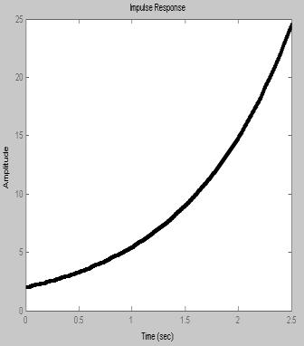
55 Transfer function X() s s A a Time-domain impulse response x() t Ae at Position of poles and zeros j -a 0 i 0 55

56 Transfer function X() s A s B ( s a) b Time-domain impulse response at x( t) Ae sin( bt ) Position of poles and zeros j b -a 0 i 0 56

57 Transfer function X() s A s B s b Time-domain impulse response x( t) Asin( bt ) Position of poles and zeros j b 0 i 0 57

58 Transfer function X() s A s a Time-domain impulse response x() t Ae at Position of poles and zeros j 0 -a i 58

59 Transfer function: X() s A s B ( s a) b Time-domain dynamic response at x( t) Ae sin( bt ) Position of poles and zeros -a b j 0 i 0 59

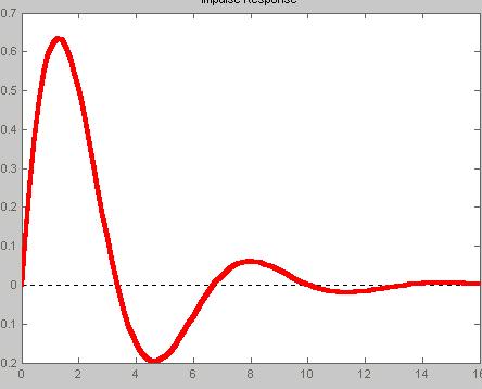
60 Summary of pole position & system dynamics 60

61 Characteristic equation -obtained by setting the denominator polynomial of the transfer function to zero n n1 s an 1s a1s a0 0 Note: stability of linear single-input, single-output systems is completely governed by the roots of the characteristic equation. 61

62 2-4 Block diagram and Signal-flow graph (SFG) 62

63 Block Diagrams In a block diagram all system variables are linked to each other through functional blocks The transfer functions of the components are usually entered in the corresponding blocks Blocks are connected by arrows to indicate the direction of the flow of signals Note: The dimension of the output signal from the block is the dimension of the input signal multiplied by the dimension of the transfer function in the block Element of a block diagram Feb-15 64

64 Block Diagrams(2) The advantage of the block diagram representation is the simplicity of forming the overall block diagram for the entire system by connecting the blocks of the components according to the signal flow A block diagram contains information concerning dynamic behavior, but it does not include any information on the physical construction of the system A number of different block diagrams can be drawn for a system Feb-15 65

65 Block Diagram Representation The transfer function relationship Y( s) G( s) U( s) can be graphically denoted through a block diagram. U(s) G(s) Y(s) Feb-15 66

66 Equivalent Transform of Block Diagram 1. Connection in series U(s) G 1 (s) X(s) G 2 (s) Y(s) U(s) G(s) Y(s) Gs ( )? Ys () G( s) G1( s) G2( s) Us () Feb-15 67

67 2. Connection in parallel U(s) G1(s) G2(s) Y1(s) Y2(s) Y(S) U(s) G(s) Y(s) Gs ( )? Ys () G( s) G1( s) G2( s) Us () Feb-15 68

68 3. Negative feedback R(s) U(s) _ Y ( s) U( s) G( s) U ( s) R( s) Y( s) H( s) G(s) Y(s) R(s) M(s) Y(s) H(s) Transfer function of a negative feedback system: Gs ( ) gain of the forward path M() s 1G( s) H( s) 1 gain of the loop Y( s) R( s) Y( s) H( s) G( s) Feb-15 69

69 Block Diagram Reduction Any number of cascaded blocks can be replaced by a single block, the transfer function of which is simply the product of the individual transfer functions Blocks can be connected in series only if the output of one block is not affected by the next following block (no feedback) A complicated block diagram involving many feedback loops can be simplified by a step-by-step rearrangement Simplification of the block diagram by rearrangements considerably reduces the labor needed for subsequent mathematical analysis Feb-15 72

70 Block Diagram Transformations Feb-15 73

71 Example Simplify this diagram Solution: By moving the summing point of the negative feedback loop containing H 2 outside the positive feedback loop containing H 1, we obtain Feb-15 74

72 Example (2) Eliminating the positive feedback loop The elimination of the loop containing H 2 /G 1 gives Finally, eliminating the feedback loop results in Feb-15 75

73 Example (3) Notice that the numerator of the closed-loop transfer function C(s)/R(s) is the product of the transfer functions of the feed-forward path. The denominator of C(s)/R(s) is equal to The positive feedback loop yields a negative term in the denominator Feb-15 76

74 Signal Flow Graph Feb-15 77

75 Signal Flow Graph (SFG) SFG was introduced by S.J. Mason for the cause-andeffect representation of linear systems. 1. Each signal is represented by a node. 2. Each transfer function is represented by a branch. U(s) G(s) Y(s) G(s) U(s) Y(s) R(s) _ U(s) G(s) Y(s) R(s) 1 U(s) G(s) Y(s) H(s) -H(s) Feb-15 78

76 Block Diagram and Signal-Flow Graph Ur () s - 1 I () s 1-1 sc R1 1 U () s 1 1 R 2 Uc I () s 2 sc 1 () s - 2 U () s I () s U () s I () s r 1 1 R1 1 sc 2 U () c s Note: A signal flow graph and a block diagram contain exactly the same information (there is no advantage to one over the other; there is only personal preference) sc R Feb-15 79

77 Mason s Rule N M k N Ys ( ) 1 M () s M k Us () k1 Total number of forward paths between output Y(s) and input U(s) Path gain of the k th forward path 1 (all individual loop gains) (gain products of all possible two loops that do not touch) (gain products of all possible three loo ps that do not touch) k Value of for that part of the block diagram that does not touch the k th forward path k Feb-15 80

78 Example 1 Find the transfer function for the following block diagram U(s) 1 + _ /s 1/s 1/s a1 b1 b2 b Y(s) + Solution: Forward path a2 Path gain 1 M1 1 ( b1)(1) s 1 1 M2 1 ( b2)(1) s s M3 1 ( b3)(1) s s s and the determinates are a1 a2 a s s s a3 Feb-15 89

79 Example 1 Find the transfer function for the following block diagram U(s) 1 + _ /s 1/s 1/s a1 b1 b2 b Y(s) + Solution: Y() s M() s U() s N k1 a2 a3 Applying Mason s rule, we find the transfer function to be M k k b s b s b s a s a s a Feb-15 90

80 Example 2 Find the transfer function for the following SFG H 4 Us () Solution: Forward path 1 H 5 H 1 Path gain M H H H 1256 M2 H4 Loop path Path gain l1 H1H5 343 l H H H H l3 H3H l4 H4H7H6H5 H 3 and the determinates are 1 l l l l ( l l ) H 7 1 HH Ys () Feb-15 91

81 Example 2 Find the transfer function for the following SFG H 4 Us () M() s 1 H 5 Y() s U() s H 1 Solution: Applying Mason s rule, we find the transfer function to be N k1 M k k H H H H H H H H H H H H H H H H H H H H H H H 2 H 3 H 7 1 Ys () Feb-15 92