CSE 167: Lecture 11: Bézier Curves. Jürgen P. Schulze, Ph.D. University of California, San Diego Fall Quarter 2012

Transcription

1 CSE 167: Introduction to Computer Graphics Lecture 11: Bézier Curves Jürgen P. Schulze, Ph.D. University of California, San Diego Fall Quarter 2012

2 Announcements Homework project #5 due Nov. 9 th at 1:30pm To be presented in lab 260 Veterans Day: reschedule homework introduction Friday at 3:30pm? Tuesday before or after class? In Winter: CSE 190: 3D User Interaction 4 Units 2 lectures (Mon/Wed 11am-12:20pm) Programming assignments for 3D input devices 2

3 Lecture Overview Polynomial Curves Introduction Polynomial functions Bézier Curves Introduction Drawing Bézier curves Piecewise Bézier curves 3

4 Modeling Creating 3D objects How to construct complex surfaces? Goal Specify objects with control points Objects should be visually pleasing (smooth) Start with curves, then generalize to surfaces Next: What can curves be used for? 4

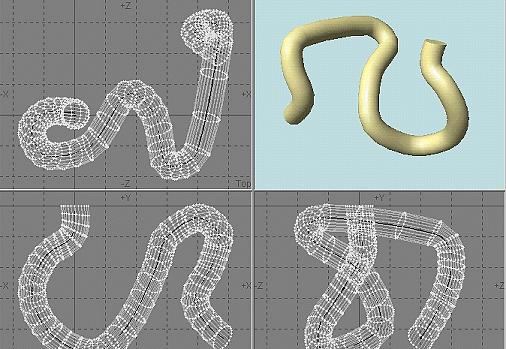
5 Curves Surface of revolution 5

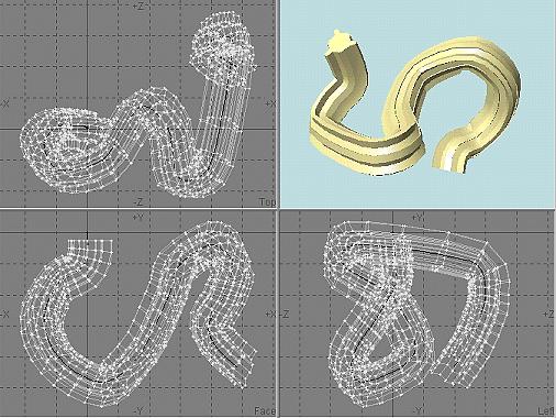
6 Curves Extruded/swept surfaces 6

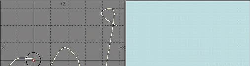
7 Curves Animation Provide a track for objects Use as camera path 7

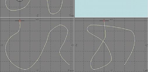
8 Curves Specify parameter values over time 8

9 Curves Can be generalized to surface patches 9

10 Curve Representation Specify many points along a curve, connect with lines? Difficult to get precise, smooth results across magnification levels Large storage and CPU requirements How many points are enough? Specify a curve using a small number of control points Known as a spline curve or just spline Control point 10

11 Spline: Definition Wikipedia: Term comes from flexible spline devices used by shipbuilders and draftsmen to draw smooth shapes. Spline consists of a long strip fixed in position at a number of points that relaxes to form a smooth curve passing through those points. 11

12 Interpolating Control Points Interpolating means that curve goes through all control points Seems most intuitive Surprisingly, not usually the best choice Hard to predict behavior Hard to get aesthetically pleasing curves 12

13 Approximating Control Points Curve is influenced by control points Various types Most common: polynomial functions Bézier spline (our main focus) B-spline (generalization of Bézier spline) NURBS (Non Uniform Rational Basis Spline): used in CAD tools 13

14 Mathematical Definition A vector valued function of one variable x(t) Given t, compute a 3D point x=(x,y,z) Could be interpreted as three functions: x(t), y(t), z(t) Parameter t moves a point along the curve x(t) z y x(0.0) x(0.5) x(1.0) x 14

15 Tangent Vector Derivative Vector x points in direction of movement Length corresponds to speed x(t) z y x (0.0) x (0.5) x (1.0) 15 x

16 Lecture Overview Polynomial Curves Introduction Polynomial functions Bézier Curves Introduction Drawing Bézier curves Piecewise Bézier curves 16

17 Polynomial Functions Linear: (1 st order) Quadratic: (2 nd order) Cubic: (3 rd order) 17

18 Polynomial Curves Linear Evaluated as: 18

19 Polynomial Curves Quadratic: (2 nd order) Cubic: (3 rd order) We usually define the curve for 0 t 1 19

20 Control Points Polynomial coefficients a, b, c, d can be interpreted as control points Remember: a, b, c, d have x,y,z components each Unfortunately, they do not intuitively describe the shape of the curve Goal: intuitive control points 20

21 Control Points How many control points? Two points define a line (1 st order) Three points define a quadratic curve (2 nd order) Four points define a cubic curve (3 rd order) k+1 points define a k-order curve Let s start with a line 21

22 First Order Curve Based on linear interpolation (LERP) Weighted average between two values Value could be a number, vector, color, Interpolate between points p 0 and p 1 with parameter t Defines a curve that is straight (first-order spline) t=0 corresponds to p 0 t=1 corresponds to p 1 t=0.5 corresponds to midpoint 22 p 0. 0<t<1 t=0. p 1 t=1 x(t) = Lerp( t, p 0, p 1 )= ( 1 t)p 0 + t p 1

23 Linear Interpolation Three equivalent ways to write it Expose different properties 1. Regroup for points p 2. Regroup for t 3. Matrix form 23

24 Weighted Average x(t) = (1 t)p 0 + (t)p 1 = B 0 (t) p 0 + B 1 (t)p 1, where B 0 (t) = 1 t and B 1 (t) = t Weights are a function of t Sum is always 1, for any value of t Also known as blending functions 24

25 Linear Polynomial x(t) = (p p 0 ) t + p vector point Curve is based at point p 0 Add the vector, scaled by t p 0..5(p 1 -p 0 ). p 1 -p 0. 25

26 Matrix Form Geometry matrix Geometric basis Polynomial basis In components 26

27 Tangent For a straight line, the tangent is constant Weighted average Polynomial Matrix form 27

28 Lecture Overview Polynomial Curves Introduction Polynomial functions Bézier Curves Introduction Drawing Bézier curves Piecewise Bézier curves 28

29 Bézier Curves Are a higher order extension of linear interpolation p 1 p 1 p 1 p 2 p 1 p 3 p 0 p 0 p 0 p 2 Linear Quadratic Cubic 29

30 Bézier Curves Give intuitive control over curve with control points Endpoints are interpolated, intermediate points are approximated Convex Hull property Variation-Diminishing property Many demo applets online, for example: Demo: ezier/bezier.html 30

31 Cubic Bézier Curve Most commonly used case Defined by four control points: Two interpolated endpoints (points are on the curve) Two points control the tangents at the endpoints Points x on curve defined as function of parameter t p 0 x(t) p 1 p 2 31 p 3

32 Algorithmic Construction Algorithmic construction De Casteljau algorithm, developed at Citroen in 1959, named after its inventor Paul de Casteljau (pronounced Cast-all- Joe ) Developed independently from Bézier s work: Bézier created the formulation using blending functions, Casteljau devised the recursive interpolation algorithm 32

33 De Casteljau Algorithm A recursive series of linear interpolations Works for any order Bezier function, not only cubic Not very efficient to evaluate Other forms more commonly used But: Gives intuition about the geometry Useful for subdivision 33

34 De Casteljau Algorithm Given: Four control points A value of t (here t 0.25) p 1 p 0 p 2 p 3 34

35 De Casteljau Algorithm p 1 q 1 q 0 (t) = Lerp( t,p 0,p ) 1 p 0 q 0 ( ) q 1 (t) = Lerp t,p 1,p 2 p 2 q 2 (t) = Lerp( t,p 2,p ) 3 q 2 p 3 35

36 De Casteljau Algorithm q 1 q r 0 0 r 1 ( ) r 0 (t) = Lerp t,q 0 (t),q 1 (t) r 1 (t) = Lerp( t,q 1 (t),q 2 (t)) q 2 36

37 De Casteljau Algorithm r 0 x r 1 x(t) = Lerp( t,r 0 (t),r 1 (t)) 37

38 De Casteljau Algorithm p 1 p 0 x p 2 Applets Demo: p 3

39 Recursive Linear Interpolation x = Lerp t,r 0,r 1 ( ) r = Lerp ( t,q,q ) ( ) r 1 = Lerp t,q 1,q 2 q 0 = Lerp( t,p 0,p ) 1 q 1 = Lerp( t,p 1,p ) 2 q 2 = Lerp( t,p 2,p ) 3 p 0 p 1 p 2 p 3 p 1 q 0 r 0 p 2 x q 1 r 1 p 3 q 2 p 4 39

40 Expand the LERPs q 0 (t) = Lerp( t,p 0,p 1 )= ( 1 t)p 0 + tp 1 q 1 (t) = Lerp( t,p 1,p 2 )= ( 1 t)p 1 + tp 2 q 2 (t) = Lerp( t,p 2,p 3 )= ( 1 t)p 2 + tp 3 r 0 (t) = Lerp ( t,q 0 (t),q 1 (t) )= 1 t r 1 (t) = Lerp( t,q 1 (t),q 2 (t))= 1 t ( ) ( )p 0 + tp 1 )+ t ( 1 t )p 1 + tp 2 ( )p 1 + tp 2 )+ t ( 1 t)p 2 + tp 3 ( ) 1 t ( ) 1 t x(t) = Lerp t,r 0 (t),r 1 (t) = ( 1 t) ( 1 t) ( 1 t)p 0 + tp 1 )+ t ( 1 t)p 1 + tp 2 +t ( 1 t) ( 1 t)p 1 + tp 2 )+ t ( 1 t)p 2 + tp 3 40 ( ) ( ) ( ) ( ) ( ) ( )

41 Weighted Average of Control Points Regroup for p: x(t) = 1 t ( )p 0 + tp 1 )+ t ( 1 t)p 1 + tp 2 ( )p 1 + tp 2 )+ t( 1 t)p 2 + tp 3 ) ( ) ( 1 t) 1 t +t 1 t ( ) ( ) ( ) 1 t ( ) x(t) = 1 t ( ) 3 p ( ) ( 1 t) 2 tp t ( )t 2 p 2 + t 3 p 3 B 0 (t ) B (t ) x(t) = t 3 + 3t 2 3t + 1 p 0 + 3t 3 6t 2 + 3t ( ) ( ) + 3t 3 + 3t p + t 3 2 { p 3 B 2 (t ) ( ) B 3 (t ) ( ) p 1 41

42 Cubic Bernstein Polynomials x(t) = B 0 ( t)p 0 + B 1 ( t)p 1 + B 2 ( t)p 2 + B 3 ( t)p 3 The cubic Bernstein polynomials : B 0 ( t)= t 3 + 3t 2 3t + 1 B 1 ( t)= 3t 3 6t 2 + 3t B 2 ( t)= 3t 3 + 3t 2 ( t)= t 3 B 3 B i (t) = 1 Weights B i (t) add up to 1 for any value of t 42

43 General Bernstein Polynomials B 1 0 B 1 1 ( t)= t + 1 B 2 0 ( t)= t 2 2t + 1 B 3 0 ( t)= t 3 + 3t 2 3t + 1 ( t)= t B 2 1 ( t)= 2t 2 + 2t B 3 1 ( t)= 3t 3 6t 2 + 3t B 2 2 ( t)= t 2 B 3 2 ( t)= 3t 3 + 3t 2 B 3 3 ( t)= t 3 43 B i n ( t)= n i ( 1 t)n i t B n i ( t) = 1 n ( ) i i = n! i! ( n i)! n! = factorial of n (n+1)! = n! x (n+1)

44 General Bézier Curves nth-order Bernstein polynomials form nth-order Bézier curves B i n ( t)= n ( 1 t)n i t i n i=0 x( t)= B n i ( t)p i ( ) i 44

45 Bézier Curve Properties Overview: Convex Hull property Variation Diminishing property Affine Invariance 45

46 Definitions Convex hull of a set of points: Polyhedral volume created such that all lines connecting any two points lie completely inside it (or on its boundary) Convex combination of a set of points: Weighted average of the points, where all weights between 0 and 1, sum up to 1 Any convex combination of a set of points lies within the convex hull 46

47 Convex Hull Property A Bézier curve is a convex combination of the control points (by definition, see Bernstein polynomials) A Bézier curve is always inside the convex hull Makes curve predictable Allows culling, intersection testing, adaptive tessellation Demo: p 1 p 3 p 0 p 2 47

48 Variation Diminishing Property If the curve is in a plane, this means no straight line intersects a Bézier curve more times than it intersects the curve's control polyline Curve is not more wiggly than control polyline 48

49 Affine Invariance Transforming Bézier curves Two ways to transform: Transform the control points, then compute resulting spline points Compute spline points, then transform them Either way, we get the same points Curve is defined via affine combination of points Invariant under affine transformations (i.e., translation, scale, rotation, shear) Convex hull property remains true 49

50 Cubic Polynomial Form Start with Bernstein form: x(t) = ( t 3 + 3t 2 3t + 1)p 0 + ( 3t 3 6t 2 + 3t)p 1 + ( 3t 3 + 3t 2 )p 2 + ( t 3 )p 3 Regroup into coefficients of t : x(t) = ( p 0 + 3p 1 3p 2 + p 3 )t 3 + ( 3p 0 6p 1 + 3p 2 )t 2 + ( 3p 0 + 3p 1 )t + ( p 0 )1 x(t) = at 3 + bt 2 + ct + d ( ) ( ) ( ) ( ) a = p 0 + 3p 1 3p 2 + p 3 b = 3p 0 6p 1 + 3p 2 c = 3p 0 + 3p 1 d = p 0 Good for fast evaluation Precompute constant coefficients (a,b,c,d) Not much geometric intuition 50

51 Cubic Matrix Form x(t) = a r t 3 r b c r t 2 d t 1 r a = p 0 + 3p 1 3p 2 + p 3 r b = ( 3p 0 6p 1 + 3p 2 ) r c = ( 3p 0 + 3p 1 ) d = p 0 ( ) ( ) t x(t) = [ p 0 p 1 p 2 p 3 ] t t { T G Bez B Bez Other types of cubic splines use different basis matrices B Bez 51

52 Cubic Matrix Form In 3D: 3 equations for x, y and z: 52 [ ] x x (t) = p 0 x p 1x p 2 x p 3x x y (t) = p 0 y p 1y p 2 y p 3y x z (t) = p 0z p 1z p 2z p 3z t t t t t t t t t

53 Matrix Form Bundle into a single matrix x(t) = t 3 p 0 x p 1x p 2 x p 3x p 0 y p 1y p 2 y p 3y t t p 0z p 1z p 2z p 3z x(t) = G Bez B Bez T x(t) = C T Efficient evaluation Pre-compute C Take advantage of existing 4x4 matrix hardware support 53