8. Diagonalization.

Transcription

1 8. Diagonalization

2 8.1. Matrix Representations of Linear Transformations Matrix of A Linear Operator with Respect to A Basis We know that every linear transformation T: R n R m has an associated standard matrix with the property that for every vector x in R n. For the moment we will focus on the case where T is a linear operator on R n, so the standard matrix [T] is a square matrix of size n n. Sometimes the form of the standard matrix fully reveals the geometric properties of a linear operator and sometimes it does not. Our primary goal in this section is to develop a way of using bases other than the standard basis to create matrices that describe the geometric behavior of a linear transformation better than the standard matrix.

3 8.1. Matrix Representations of Linear Transformations Matrix of A Linear Operator with Respect to A Basis Suppose that is a linear operator on R n and B is a basis for R n. In the course of mapping x into T(x) this operator creates a companion operator that maps the coordinate matrix [x] B into the coordinate matrix [T(x)] B. There must be a matrix A such that

4 8.1. Matrix Representations of Linear Transformations Matrix of A Linear Operator with Respect to A Basis Let x be any vector in R n, and suppose that its coordinate matrix with respect to B is That is,

5 8.1. Matrix Representations of Linear Transformations Matrix of A Linear Operator with Respect to A Basis It now follows from the linearity of T that and from the linearity of coordinate maps that which we can write in matrix form as This proves that the matrix A in (4) has property (5). Moreover, A is the only matrix with this property, for if there exists a matrix C such that for all x in R n, then Theorem implies that A=C.

6 8.1. Matrix Representations of Linear Transformations Matrix of A Linear Operator with Respect to A Basis The matrix A in (4) is called the matrix for T with respect to the basis B and is denoted by Using this notation we can write (5) as

7 8.1. Matrix Representations of Linear Transformations Matrix of A Linear Operator with Respect to A Basis Example 1 Let T: R 2 R 2 be the linear operator whose standard matrix is Find the matrix for T with respect to the basis B={v 1,v 2 }, where The images of the basis vectors under the operator T are

8 8.1. Matrix Representations of Linear Transformations Matrix of A Linear Operator with Respect to A Basis Example 1 so the coordinate matrices of these vectors with respect to B are Thus, it follows from (6) that This matrix reveals geometric information about the operator T that was not evident from the standard matrix. It tells us that the effect of T is to stretch the v 2 -coordinate of a vector by a factor of 5 and to leave the v 1 -coordinate unchanged.

9 8.1. Matrix Representations of Linear Transformations Matrix of A Linear Operator with Respect to A Basis Example 2 Let T: R 3 R 3 be the linear operator whose standard matrix is We showed in Example 7 of Section 6.2 that T is a rotation through an angle 2π/3 about an axis in the direction of the vector n=(1,1,1). Let us now consider how the matrix for T would look with respect to an orthonormal basis B={v 1,v 2,v 3 } in which v 3 =v 1 v 2 is a positive scalar multiple of n and {v 1,v 2 } is an orthonormal basis for the plane W through the origin that is perpendicular to the axis of rotation.

10 8.1. Matrix Representations of Linear Transformations Matrix of A Linear Operator with Respect to A Basis Example 2 The rotation leaves the vector v 3 fixed, so and hence Also, T(v 1 ) and T(v 2 ) are linear combinations of v 1 and v 2, since these vectors lie in W. This implies that the third coordinate of both [T(v 1 )] B and [T(v 2 )] B must be zero, and the matrix for T with respect to the basis B must be of the form

11 8.1. Matrix Representations of Linear Transformations Matrix of A Linear Operator with Respect to A Basis Example 2 Since T behaves exactly like a rotation of R 2 in the plane W, the block of missing entries has the form of a rotation matrix in R 2. Thus,

12 8.1. Matrix Representations of Linear Transformations Changing Bases Suppose that T: R n R n is a linear operator and that B={v 1,v 2,,v n } and B ={v 1,v 2,,v n } are bases for R n. Also, let P=P B B be the transition matrix from B to B (so P -1 =P B B is the transition matrix from B to B). The diagram shows two different paths from [x] B to [T(x)] B : 1. (10) 2. (11) Thus, (10) and (11) together imply that Since this holds for all x in R n, it follows from Theorem that

13 8.1. Matrix Representations of Linear Transformations Changing Bases When convenient, Formula (12) can be rewritten as and in the case where the bases are orthonormal this equation can be expressed as

14 8.1. Matrix Representations of Linear Transformations Changing Bases Since many linear operators are defined by their standard matrices, it is important to consider the special case of Theorem in which B =S is the standard basis for R n. In this case [T] B =[T] S =[T], and the transition matrix P from B to B has the simplified form

15 8.1. Matrix Representations of Linear Transformations Changing Bases When convenient, Formula (17) can be rewritten as and in the case where B is an orthonormal basis this equation can be expressed as

16 8.1. Matrix Representations of Linear Transformations Changing Bases Formula (17) [or (19) in the orthogonal case] tells us that the process of changing from the standard basis for R n to a basis B produces a factorization of the standard matrix for T as in which P is the transition matrix from the basis B to the standard basis S. To understand the geometric significance of this factorization, let us use it to compute T(x) by writing Reading from right to left, this equation tells us that T(x) can be obtained by first mapping the standard coordinates of x to B-coordinates using the matrix P -1, then performing the operation on the B-coordinates using the matrix [T] B, and then using the matrix P to map the resulting vector back to standard coordinates.

17 8.1. Matrix Representations of Linear Transformations Changing Bases Example 3 In Example 1 we considered the linear operator T: R 2 R 2 whose standard matrix is and we showed that with respect to the orthonormal basis B={v 1,v 2 } that is formed from the vectors

18 8.1. Matrix Representations of Linear Transformations Changing Bases Example 3 In this case the transition matrix from B to S is so it follows from (17) that [T] can be factored as

19 8.1. Matrix Representations of Linear Transformations Changing Bases Example 4 In Example 2 we considered the rotation T: R 3 R 3 whose standard matrix is and we showed that From Example 7 of Section 6.2, the equation of the plane W is From Example 10 of Section 7.9, an orthonormal basis for the plane is

20 8.1. Matrix Representations of Linear Transformations Changing Bases Example 4 Since v 3 =v 1 v 2, The transition matrix from B={v 1,v 2,v 3 } to the standard basis is Since this matrix is orthogonal, it follows from (19) that [T] can be factored as

21 8.1. Matrix Representations of Linear Transformations Changing Bases Example 5 From Formula (2) of Section 6.2, the standard matrix for the reflection T of R 2 about the line L through the origin making an angle θ with the positive x-axis of a rectangular xy-coordinate system is Suppose that we rotate the coordinate axes through the angle θ to align the new x -axis with L, and we let v 1 and v 2 be unit vectors along the x - and y -axes, respectively. Since and it follows that the matrix for T with respect to the basis B={v 1,v 2 } is

22 8.1. Matrix Representations of Linear Transformations Changing Bases Example 5 Also, it follows from Example 8 of Section 7.11 that the transition matrices between the standard basis S and the basis B are Thus, Formula (19) implies that

23 8.1. Matrix Representations of Linear Transformations Matrix of A Linear Transformation with Respect to A Pair of Bases Recall that every linear transformation T: R n R m has an associated m n standard matrix with the property that If B and B are bases for R n and R m, respectively, then the transformation creates an associated transformation that maps the coordinate matrix [x] B into the coordinate matrix [T(x)] B. As in the operator case, this associated transformation is linear and hence must be a matrix transformation; that is, there must be a matrix A such that

24 8.1. Matrix Representations of Linear Transformations Matrix of A Linear Transformation with Respect to A Pair of Bases The matrix A in (23) is called the matrix for T with respect to the bases B and B and is denoted by the symbol [T] B,B.

25 8.1. Matrix Representations of Linear Transformations Matrix of A Linear Transformation with Respect to A Pair of Bases Example 6 Let T: R 2 R 3 be the linear transformation defined by Find the matrix for T with respect to the bases B={v 1,v 2 } for R 2 and B ={v 1,v 2,v 3 } for R 3, where Using the given formula for T we obtain

26 8.1. Matrix Representations of Linear Transformations Matrix of A Linear Transformation with Respect to A Pair of Bases Example 6 and expressing these vectors as linear combinations of v 1, v 2, and v 3 we obtain Thus,

27 8.1. Matrix Representations of Linear Transformations Effect of Changing Bases on Matrices of Linear Transformations In particular, if B 1 and B 1 are the standard bases for R n and R m, respectively, and if B and B are any bases for R n and R m, respectively, then it follows from (27) that where U is the transition matrix from B to the standard basis for R n and V is the transition matrix from B to the standard basis for R m.

28 8.1. Matrix Representations of Linear Transformations Representing Linear Operators with Two Bases The single-basis representation of T with respect to B can be viewed as the two-basis representation in which both bases are B.

29 8.2. Similarity and Diagonalizability Similar Matrices REMARK If C is similar to A, then it is also true that A is similar to C. You can see this by letting Q=P -1 and rewriting the equation C=P -1 AP as

30 8.2. Similarity and Diagonalizability Similar Matrices Let T: R n R n denote multiplication by A; that is, (1) As A and C are similar, there exists an invertible matrix P such that C=P -1 AP, so it follows from (1) that (2) If we assume that the column-vector form of P is then the invertibility of P and Theorem imply that B={v 1,v 2,,v n } is a basis for R n. It now follows from Formula (2) above and Formula (20) of Section 8.1 that

31 8.2. Similarity and Diagonalizability Similarity Invariants There are a number of basic properties of matrices that are shared by similar matrices. For example, if C=P -1 AP, then which shows that similar matrices have the same determinant. In general, any property that is shared by similar matrices is said to be a similarity invariant.

32 8.2. Similarity and Diagonalizability Similarity Invariants (e) If A and C are similar matrices, then so are and for any scalar λ. This shows that and are similar, so (3) now follows from part (a). (3)

33 8.2. Similarity and Diagonalizability Similarity Invariants Example 1 Show that there do not exist bases for R2 with respect to which the matrices and Represent the same linear operator. For A and C to represent the same linear operator, the two matrices would have to be similar by Theorem But this cannot be, since tr(a)=7 and tr(c)=5, contradicting the fact that the trace is a similarity invariant.

34 8.2. Similarity and Diagonalizability Eigenvectors and Eigenvalues of Similar Matrices Recall that the solution space of is called the eigenspace of A corresponding to λ 0. We call the dimension of this solution space the geometric multiplicity of λ 0. Do not confuse this with the algebraic multiplicity of λ 0, which is the number of repetition of the factor λ-λ 0 in the complete factorization of the characteristic polynomial of A.

35 8.2. Similarity and Diagonalizability Eigenvectors and Eigenvalues of Similar Matrices Example 2 Find the algebraic and geometric multiplicities of the eigenvalues of λ=2 has algebraic multiplicity 1 λ=3 has algebraic multiplicity 2 One way to find the geometric multiplicities of the eigenvalues is to find bases for the eigenspaces and then determine the dimensions of those spaces from the number of basis vectors.

36 8.2. Similarity and Diagonalizability Eigenvectors and Eigenvalues of Similar Matrices Example 2 If λ=2, If λ=3, λ=2 has algebraic multiplicity 1, geometric multiplicity 1 λ=3 has algebraic multiplicity 2, geometric multiplicity 1

37 8.2. Similarity and Diagonalizability Eigenvectors and Eigenvalues of Similar Matrices Example 3 Find the algebraic and geometric multiplicities of the eigenvalues of λ=1 has algebraic multiplicity 1 λ=2 has algebraic multiplicity 2

38 8.2. Similarity and Diagonalizability Eigenvectors and Eigenvalues of Similar Matrices Example 3 If λ=1, If λ=2, λ=1 has algebraic multiplicity 1, geometric multiplicity 1 λ=2 has algebraic multiplicity 2, geometric multiplicity 2

39 8.2. Similarity and Diagonalizability Eigenvectors and Eigenvalues of Similar Matrices Let us assume first that A and C are similar matrices. Since similar matrices have the same characteristics polynomial, it follows that A and C have the same eigenvalues with the same algebraic multiplicities. To show that an eigenvalue has the same geometric multiplicity for both matrices, we must show that the solution spaces of and have the same dimension, or equivalently, that the matrices and have the same nullity. (12) But we showed in the proof of Theorem that the similarity of A and C implies the similarity of the matrices in (12). Thus, these matrices have the same nullity by part (c) of Theorem

40 8.2. Similarity and Diagonalizability Eigenvectors and Eigenvalues of Similar Matrices Assume that x is an eigenvector of C corresponding to λ, so x 0 and Cx= λx. If we substitute P -1 AP for C, we obtain which we can rewrite as or equivalently, (13) Since P is invertible and x 0, it follows that Px 0. Thus, the second equation in (13) implies that Px is an eigenvector of A corresponding to λ.

41 8.2. Similarity and Diagonalizability Diagonalization Diagonal matrices play an important role in may applications because, in many respects, they represent the simplest kinds of linear operators. Multiplying x by D has the effect of scaling each coordinate of w (with a sign reversal for negative d s).

42 8.2. Similarity and Diagonalizability Diagonalization We will show first that if the matrix A is diagonalizable, then it has n linearly independent eigenvector. The diagonalizability of A implies that there is an invertible matrix P and a diagonal matrix D, say and (14) such that P -1 AP=D. If we rewrite this as AP=PD and substitute (14), we obtain

43 8.2. Similarity and Diagonalizability Diagonalization Thus, if we denote the column vectors of P by p 1, p 2,, p n, then the left side of (15) can be expressed as and the right side of (15) as It follows from (16) and (17) that (17) (16) and it follows from the invertibility of P that p 1, p 2,, p n are nonzero, so we have shown that p 1, p 2,, p n are eigenvectors of A corresponding to λ 1, λ 2,, λ n, respectively. Moreover, the invertibility of P also implies that p 1, p 2,, p n are linearly independent (Theorem applied to P), so the column vectors of P form a set of n linearly independent eigenvectors of A.

44 8.2. Similarity and Diagonalizability Diagonalization Conversely, assume that A has n linearly independent eigenvectors, p 1, p 2,, p n, and that the corresponding eigenvalues are λ 1, λ 2,, λ n,so If we now form the matrices and then we obtain However, the matrix P is invertible, since its column vectors are linearly independent, so it follows from this computation that D=P -1 AP, which shows that A is diagonalizable.

45 8.2. Similarity and Diagonalizability A Method for Diagonalizing A Matrix

46 8.2. Similarity and Diagonalizability A Method for Diagonalizing A Matrix Example 4 We showed in Example 3 that the matrix has eigenvalues λ=1 and λ=2 and that basis vectors for these eigenspaces are and It is a straightforward matter to show that these three vectors are linearly independent, so A is diagonalizable and is diagonalized by

47 8.2. Similarity and Diagonalizability A Method for Diagonalizing A Matrix As a check, REMARK There is no preferred order for the columns of a diagonalizing matrix P the only effect of changing the order of the column is to change the order in which the eigenvalues appear along the main diagonal of D=P -1 AP.

48 8.2. Similarity and Diagonalizability A Method for Diagonalizing A Matrix Example 5 We showed in Example 2 that the matrix has eigenvalues λ=2 and λ=3 and that bases for the corresponding eigenspaces are and A is not diagonalizable since all other eigenvectors must be scalar multiples of one of these two.

49 8.2. Similarity and Diagonalizability Linearly Independence of Eigenvectors Example 6 The 3 3 matrix is diagonalizable, since it has three distinct eigenvalues, λ=2, λ=3, and λ=4. The converse of Theorem is false; that is, it is possible for an n n matrix to be diagonalizable without having n distinct eigenvalues.

50 8.2. Similarity and Diagonalizability Linearly Independence of Eigenvectors The key to diagonalizability rests with the dimensions of the eigenspaces. Example 7 Eigenvalues λ=2 and λ=3 λ=1 and λ=2 Geometric multiplicities Diagonalizable X O

51 8.2. Similarity and Diagonalizability Relationship between Algebraic and Geometric Multiplicity The geometric multiplicity of an eigenvalue cannot exceed its algebraic multiplicity. For example, if the characteristic polynomial of some 6 6 matrix A is The eigenspace corresponding to λ=6 might have dimension 1, 2, or 3, the eigenspace corresponding to λ=5 might have dimension 1 or 2, and the eigenspace corresponding to λ=3 must have dimension 1.

52 8.2. Similarity and Diagonalizability A Unifying Theorem on Diagonalizability

53 8.3. Orthogonal Diagonalizability; Functions of a Matrix Orthogonal Similarity Two n n matrices A and C are said to be similar if there exists an invertible matrix P such that C=P -1 AP. If C is orthogonally similar to A, then A is orthogonally similar to C, so we will usually say that A and C are orthogonally similar.

54 8.3. Orthogonal Diagonalizability; Functions of a Matrix Orthogonal Similarity

55 8.3. Orthogonal Diagonalizability; Functions of a Matrix Orthogonal Similarity Suppose that (1) where P is orthogonal and D is diagonal. Since P T P=PP T =I, we can rewrite (1) as Transposing both sides of this equation and using the fact that D T =D yields which shows that an orthogonally diagonalizable matrix must be symmetric.

56 8.3. Orthogonal Diagonalizability; Functions of a Matrix Orthogonal Similarity The orthogonal diagonalizability of A implies that there exists an orthogonal matrix P and a diagonal matrix D such that P T AP=D. However, since the column vectors of an orthogonal matrix are orthonormal, and since the column vectors of P are eigenvectors of A (see the proof of Theorem 8.2.6), we have established that the column vectors of P form an orthonormal set of n eigenvectors of A. Conversely, assume that there exists an orthonormal set {p 1, p 2,, p n } of n eigenvectors of A. We showed in the proof of Theorem that the matrix diagonalizes A. However, in this case P is an orthogonal matrix, since its column vectors are orthonormal. Thus, P orthogonally diagonalizes A.

57 8.3. Orthogonal Diagonalizability; Functions of a Matrix Orthogonal Similarity (b) Let v 1 and v 2 be eigenvectors corresponding to distinct eigenvalues λ 1 and λ 2, respectively. The proof that v 1 v 2 =0 will be facilitated by using Formula (26) of Section 3.1 to write λ 1 (v 1 v 2 )=(λ 1 v 1 ) v 2 as the matrix product (λ 1 v 1 ) T v 2. The rest of the proof now consists of manipulating this expression in the right way: [v 1 is an eigenvector corresponding to λ 1 ] [symmetry of A] [v 2 is an eigenvector corresponding to λ 2 ] [Formula (26) of Section 3.1] This implies that (λ 1 - λ 2 )(v 1 v 2 )=0, so v 1 v 2 =0 as a result of the fact that λ 1 λ 2.

58 8.3. Orthogonal Diagonalizability; Functions of a Matrix A Method for Orthogonally Diagonalizing A Symmetric Matrix

59 8.3. Orthogonal Diagonalizability; Functions of a Matrix A Method for Orthogonally Diagonalizing A Symmetric Matrix Example 1 Find a matrix P that orthogonally diagonalizes the symmetric matrix The characteristic equation of A is Thus, the eigenvalues of A are λ=2 and λ=8. Using the method given in Example 3 of Section 8.2, it can be shown that the vectors and form a basis for the eigenspace corresponding to λ=2 and that

60 8.3. Orthogonal Diagonalizability; Functions of a Matrix A Method for Orthogonally Diagonalizing A Symmetric Matrix Example 1 is a basis for the eigenspace corresponding to λ=8. Applying the Gram-Schmidt process to the bases {v 1, v 2 } and {v 3 } yields the orthonormal bases {u 1, u 2 } and {u 3 }, where and Thus, A is orthogonally diagonalized by the matrix

61 8.3. Orthogonal Diagonalizability; Functions of a Matrix A Method for Orthogonally Diagonalizing A Symmetric Matrix Example 1 As a check,

62 8.3. Orthogonal Diagonalizability; Functions of a Matrix Spectral Decomposition If A is a symmetric matrix that is orthogonally diagonalized by and if λ 1, λ 2,, λ n are the eigenvalues of A corresponding to u 1, u 2,, u n, then we know that D=P T AP, where D is a diagonal matrix with the eigenvalues in the diagonal positions. It follows from this that the matrix A can be expressed as Multiplying out using the column-row rule (Theorem 3.8.1), we obtain the formula which is called a spectral decomposition of A or an eigenvalue decomposition of A (sometimes abbreviated as the EVD of A).

63 8.3. Orthogonal Diagonalizability; Functions of a Matrix Spectral Decomposition Example 2 The matrix has eigenvalues λ 1 =-3 and λ 2 =2 with corresponding eigenvectors and Normalizing these basis vectors yields and so a spectral decomposition of A is

64 8.3. Orthogonal Diagonalizability; Functions of a Matrix Spectral Decomposition Example 2 where the 2 2 matrices on the right are the standard matrices for the orthogonal projections onto the eigenspaces. Now let us see what this decomposition tells us about the image of the vector x=(1,1) under multiplication by A. Writing x in column form, it follows that and from (6) that (7) (6) (8)

65 8.3. Orthogonal Diagonalizability; Functions of a Matrix Spectral Decomposition Example 2 It follows from (7) that the image of (1,1) under multiplication by A is (3,0), and it follows from (8) that this image can also be obtained by projecting (1,1) onto the eigenspaces corresponding to λ 1 =-3 and λ 2 =2 to obtain vectors and, then scaling by the eigenvalues to obtain and, and then adding these vectors.

66 8.3. Orthogonal Diagonalizability; Functions of a Matrix Powers of A Diagonalizable Matrix Suppose that A is an n n matrix and P is an invertible n n matrix. Then and more generally, if k is any positive integer, then (9) In particular, if A is diagonalizable and P -1 AP=D is a diagonal matrix, then it follows from (9) that which we can rewrite as (11)

67 8.3. Orthogonal Diagonalizability; Functions of a Matrix Powers of A Diagonalizable Matrix Example 3 Use Formula (11) to find A 13 for the diagonalizable matrix We showed in Example 4 of Section 8.2 that Thus,

68 8.3. Orthogonal Diagonalizability; Functions of a Matrix Powers of A Diagonalizable Matrix In the special case where A is a symmetric matrix with a spectral decomposition the matrix orthogonally diagonalizes A, so (11) can be expressed as This equation can be written as from which it follows that A k is a symmetric matrix whose eigenvalues are the kth powers of the eigenvalues of A.

69 8.3. Orthogonal Diagonalizability; Functions of a Matrix Cayley-Hamilton Theorem The Cayley-Hamilton theorem makes it possible to express all positive integer powers of an n n matrix A in terms of I, A,, A n-1 by solving (14) of A n. In the case where A is invertible, it also makes it possible to express A -1 (and hence all negative powers of A) in terms of I, A,, A n-1 by rewriting (14) as, from which it follows that A -1 is the parenthetical expression on the left.

70 8.3. Orthogonal Diagonalizability; Functions of a Matrix Cayley-Hamilton Theorem Example 4 We showed in Example 2 of Section 8.2 that the characteristic polynomial of is so the Cayley-Hamilton theorem implies that This equation can be used to express A 3 and all higher powers of A in terms of I, A, and A 2. For example, (16)

71 8.3. Orthogonal Diagonalizability; Functions of a Matrix Cayley-Hamilton Theorem Example 4 and using this equation we can write Equation (16) can also be used to express A -1 as a polynomial in A by rewriting it as from which it follows that

72 8.3. Orthogonal Diagonalizability; Functions of a Matrix Exponential of A Matrix In Section 3.2 we defined polynomial functions of square matrices. Recall from that discussion that if A is an n n matrix and then the matrix p(a) is defined as

73 8.3. Orthogonal Diagonalizability; Functions of a Matrix Exponential of A Matrix Other functions of square matrices can be defined using power series. For example, if the function f is represented by its Maclaurin series on some interval, then we define f(a) to be (18) where we interpret this to mean that the ijth entry of f(a) is the sum of the series of the ijth entries of the terms on the right.

74 8.3. Orthogonal Diagonalizability; Functions of a Matrix Exponential of A Matrix In the special case where A is a diagonal matrix, say and f is defined at the point d 1, d 2,, d k, each matrix on the right side of (18) is diagonal, and hence so is f(a). In this case, equating corresponding diagonal entries on the two sides of (18) yields

75 8.3. Orthogonal Diagonalizability; Functions of a Matrix Exponential of A Matrix Thus, we can avoid the series altogether in the diagonal case and compute f(a) directly as For example, if, then

76 8.3. Orthogonal Diagonalizability; Functions of a Matrix Exponential of A Matrix If A is an n n diagonalizable matrix and P -1 AP=D, where then (10) and (18) suggest that This tells us that f(a) can be expressed as

77 8.3. Orthogonal Diagonalizability; Functions of a Matrix Exponential of A Matrix

78 8.3. Orthogonal Diagonalizability; Functions of a Matrix Exponential of A Matrix Example 5 Find e ta for the diagonalizable matrix We showed in Example 4 of Section 8.2 that

79 8.3. Orthogonal Diagonalizability; Functions of a Matrix Exponential of A Matrix Example 5 so applying Formula (21) with f(a)=e ta implies that

80 8.3. Orthogonal Diagonalizability; Functions of a Matrix Exponential of A Matrix In the special case where A is a symmetric matrix with a spectral decomposition the matrix orthogonally diagonalizes A, so (20) can be expressed as This equation can be written as, which tells us that f(a) is a symmetric matrix whose eigenvalues can be obtained by evaluating f at the eigenvalues of A.

81 8.3. Orthogonal Diagonalizability; Functions of a Matrix Diagonalization and Linear Systems Assume that we are solving a linear system Ax=b. Suppose that A is diagonalizable and P -1 AP=D. If we define a new vector y=p -1 x, and if we substitute (23) in Ax=b, then we obtain a new linear system APy=b in the unknown y. Multiplying both sides of this equation by P -1 and using the fact that P -1 AP=D yields Since this system has a diagonal coefficient matrix, the solution for y can be read off immediately, and the vector x can then be computed using (23). Many algorithms for solving large-scale linear systems are based on this idea. Such algorithms are particularly effective in cases in which the coefficient matrix can be orthogonally diagonalized since multiplication by orthogonal matrices does not magnify roundoff error.

82 8.3. Orthogonal Diagonalizability; Functions of a Matrix The Nondiagonalizable Case In cases where A is not diagonalizable it is still possible to achieve considerable simplification in the form of P -1 AP by choosing the matrix P appropriately.

83 8.3. Orthogonal Diagonalizability; Functions of a Matrix The Nondiagonalizable Case In many numerical LU- and QR-algorithms in initial matrix is first converted to upper Hessenberg form, thereby reducing the amount of computation in the algorithm itself.

84 8.4. Quadratic Forms Definition of Quadratic Form A linear form on R n A quadratic form on R n A general quadratic form on R 2 The term of the form a k x i x j are called cross product terms. A general quadratic form on R 3

85 8.4. Quadratic Forms Definition of Quadratic Form In general, if A is a symmetric n n matrix and x is an n 1 column vector of variables, then we call the function (3) the quadratic form associated with A. When convenient, (3) can be expressed in dot product notation as

86 8.4. Quadratic Forms Definition of Quadratic Form In the case where A is a diagonal matrix, the quadratic form Q A has no cross product terms; for example, if A is the n n identity matrix, then and if A has diagonal entries λ 1, λ 2,, λ n, then

87 8.4. Quadratic Forms Definition of Quadratic Form Example 1 In each part, express the quadratic form in the matrix notation x T Ax, where A is symmetric.

88 8.4. Quadratic Forms Change of Variable in A Quadratic Form We can simplify the quadratic form x T Ax by making a substitution that expresses the variable x 1, x 2,, x n in terms of new variable y 1, y 2,, y n. If P is invertible, then we call (5) a change of variable, and if P is orthogonal, we call (5) an orthogonal change of variable. If we make the change of variable x=py in the quadratic form x T Ax, then we obtain The matrix B=P T AP is symmetric, so the effect of the change of variable is to produce a new quadratic form y T By in the variable y 1, y 2,, y n.

89 8.4. Quadratic Forms Change of Variable in A Quadratic Form In particular, if we choose P to orthogonally diagonalize A, then the new quadratic from will be y T Dy, where D is a diagonal matrix with the eigenvalues of A on the main diagonal; that is

90 8.4. Quadratic Forms Change of Variable in A Quadratic Form Example 2 Find an orthogonal change of variable that eliminates the cross product terms in the quadratic form Q=x 12 -x 32-4x 1 x 2 +4x 2 x 3, and express Q in terms of the new variables. The characteristic equation of the matrix A is so the eigenvalues are λ=0, -3, 3. the orthonormal bases for the three eigenspaces are

91 8.4. Quadratic Forms Change of Variable in A Quadratic Form Example 2 Thus, a substitution x=py that eliminates the cross product terms is This produces the new quadratic form

92 8.4. Quadratic Forms Quadratic Forms in Geometry Recall that a conic section or conic is a curve that results by cutting a double-napped cone with a plane. The most important conic sections are ellipse, hyperbolas, and parabolas, which occur when the cutting plane does not pass through the vertex. If the cutting plane passes through the vertex, then the resulting intersection is called a degenerate conic. The possibilities are a point, a pair of intersecting lines, or a single line. circle ellipse parabola hyperbola

93 8.4. Quadratic Forms Quadratic Forms in Geometry conic section central conic central conic in standard position standard forms of nondegenerate central conic

94 8.4. Quadratic Forms Quadratic Forms in Geometry A central conic whose equation has a cross product term results by rotating a conic in standard position about the origin and hence is said to rotated out of standard position. Quadratic forms on R3 arise in the study of geometric objects called quadratic surfaces (or quadrics). The most important surfaces of this type have equations of the form in which a, b, and c are not all zero. These are called central quadrics.

95 8.4. Quadratic Forms Identifying Conic Sections It is an easy matter to identify central conics in standard position by matching the equation with one of the standard forms. For example, the equation can be rewritten as which, by comparison with Table 8.4.1, is the ellipse shown in Figure

96 8.4. Quadratic Forms Identifying Conic Sections If a central conic is rotated out of standard position, then it can be identified by first rotating the coordinate axes to put it in standard position and then matching the resulting equation with one of the standard forms in Table (12) To rotate the coordinate axes, we need to make an orthogonal change of variable in which det(p)=1, and if we want this rotation to eliminate the cross product term, we must choose P to orthogonally diagonalize A. If we make a change of variable with these two properties, then in the rotated coordinate system Equation (12) will become (13) where λ 1 and λ 2 are the eigenvalues of A. the conic can now be identified by writing (13) in the form

97 8.4. Quadratic Forms Identifying Conic Sections The first column vector of P, which is a unit eigenvector corresponding to λ 1, is along the positive x -axis; and the second column vector of P, which is eigenvector corresponding to λ 2, is a unit vector along the y -axis. These are called the principal axes of the ellipse. Also, since P is the transition matrix from x y -coordinates to xy-coordinates, it follows from Formula (29) of Section 7.11 that the matrix P can be expressed in terms of the rotating angle θ as

98 8.4. Quadratic Forms Identifying Conic Sections Example 3 (a) Identify the conic whose equation is 5x 2-4xy+8y 2-36=0 by rotating the xy-axes to put the conic in standard position. (b) Find the angle θ through which you rotated the xy-axes in part (a). where The characteristic polynomial of A is Thus, A is orthogonally diagonalized by det(p)=1. If det(p)=-1, then we would have exchanged the columns to reverse the sign.

99 8.4. Quadratic Forms Identifying Conic Sections Example 3 The equation of the conic in the x y -coordinate system is which we can write as or Thus,

100 8.4. Quadratic Forms Positive Definite Quadratic Forms

101 8.4. Quadratic Forms Positive Definite Quadratic Forms It follows from the principal axes theorem (Theorem 8.4.1) that there is an orthogonal change of variable x=py for which Moreover, it follows from the invertibility of P that y 0 if and only if x 0, so the values of x T Ax for x 0 are the same as the values of y T Dy for y 0.

102 8.4. Quadratic Forms Classifying Conic Sections Using Eigenvalues x T Bx=k k 1 - an ellipse if λ 1 >0 and λ 2 >0 - no graph if λ 1 <0 and λ 2 <0 - a hyperbola if λ 1 and λ 2 have opposite signs

103 8.4. Quadratic Forms Identifying Positive Definite Matrices It can be used to determine whether a symmetric matrix is positive definite without finding the eigenvalues. Example 5 The matrix is positive definite since the determinants Thus, we are guaranteed that all eigenvalues of A are positive and x T Ax>0 for x 0.

104 8.4. Quadratic Forms Identifying Positive Definite Matrices (a) (b) Since A is symmetric, it is orthogonally diagonalizable. This means that there is an orthogonal matrix P such that P T AP=D, where D is a diagonal matrix whose entries are the eigenvalues of A. Moreover, since A is positive definite, its eigenvalues are positive, so we can write D as D=D 12, where D 1 is the diagonal matrix whose entries are the square roots of the eigenvalues of A. Thus, we have P T AP=D 12, which we can rewrite as where B=PD 1 P T.

105 8.4. Quadratic Forms Identifying Positive Definite Matrices The eigenvalues of B are the same as the eigenvalues of D 1, since eigenvalues are a similarity invariant and B is similar to D 1. Thus, the eigenvalues of B are positive, since they are the square roots of the eigenvalues of A. (b) (c) Assume that A=B 2, where B is symmetric and positive definite. Then A=B 2 =BB=BTB, so take C=B. (c) (a) Assume that A=C T C, where C is invertible. But the invertibility of C implies that Cx 0 if x 0, so x T Ax>0 for x 0.

106 8.5. Application of Quadratic Forms to Optimization Relative Extrema of Functions of Two Variables If a function f(x,y) has first partial derivatives, then its relative maxima and minima, if any, occur at points where and These are called critical points of f. The specific behavior of f at a critical point (x 0,y 0 ) is determined by the sign of If D(x,y)>0 at points (x,y) that are sufficiently close to, but different from, (x 0,y 0 ), then f(x 0,y 0 )<f(x,y) at such points and f is said to have a relative minimum at (x0,y0).

107 8.5. Application of Quadratic Forms to Optimization Relative Extrema of Functions of Two Variables If D(x,y)<0 at points (x,y) that are sufficiently close to, but different from, (x 0,y 0 ), then f(x 0,y 0 )>f(x,y) at such points and f is said to have a relative maximum at (x0,y0). If D(x,y) has both positive and negative values inside every circle centered at (x 0,y 0 ), then there are points (x,y) that are arbitrarily close to (x 0,y 0 ) at which f(x 0,y 0 )>f(x,y). In this case we say that f has a saddle point at (x 0,y 0 ).

108 8.5. Application of Quadratic Forms to Optimization Relative Extrema of Functions of Two Variables

109 8.5. Application of Quadratic Forms to Optimization Relative Extrema of Functions of Two Variables To express this theorem in terms of quadratic forms, we consider the matrix which is called the Hessian or Hessian matrix of f. The Hessian is of interest because is the expression that appears in Theorem

110 8.5. Application of Quadratic Forms to Optimization Relative Extrema of Functions of Two Variables (a) If H is positive definite, then Theorem implies that the principal submatrices of H have positive determinants. Thus, and

111 8.5. Application of Quadratic Forms to Optimization Relative Extrema of Functions of Two Variables Example 1 Find the critical points of the function and use the eigenvalues of the Hessian matrix at those points to determine which of them, if any, are relative maxima, relative minima, or saddle points. Thus, the Hessian matrix is

112 8.5. Application of Quadratic Forms to Optimization Relative Extrema of Functions of Two Variables Example 1 x=0 or y=4 We have four critical points: Evaluating the Hessian matrix at these points yields

113 8.5. Application of Quadratic Forms to Optimization Constrained Extremum Problems Geometrically, the problem of finding the maximum and minimum values of x T Ax subject to the constraint x =1 amounts to finding the highest and lowest points on the intersections of the surface with the right circular cylinder determined by the circle.

114 8.5. Application of Quadratic Forms to Optimization Constrained Extremum Problems Since A is symmetric, the principal axes theorem (Theorem 8.4.1) implies that there is an orthogonal change of variable x=py such that in which λ 1, λ 2,, λ n are the eigenvalues of A. Let us assume that x =1 and that the column vectors of P (which are unit eigenvectors of A) have been ordered so that (7) (6)

115 8.5. Application of Quadratic Forms to Optimization Constrained Extremum Problems Since P is an orthogonal matrix, multiplication by P is length preserving, so y = x =1; that is, It follows from this equation and (7) that and hence from (6) that This shows that all values of x T Ax for which x =1 lie between the largest and smallest eigenvalues of A. Let x be a unit eigenvector corresponding to λ 1. Then If x is a unit eigenvector corresponding to λ n. Then

116 8.5. Application of Quadratic Forms to Optimization Constrained Extremum Problems Example 2 Find the maximum and minimum values of the quadratic form subject to the constraint x 2 +y 2 =1 Thus, the constrained extrema are

117 8.5. Application of Quadratic Forms to Optimization Constrained Extremum Problems Example 3 A rectangle is to be inscribed in the ellipse 4x 2 +9y 2 =36, as shown in Figure Use eigenvalue methods to find nonnegative values of x and y that produce the inscribed rectangle with maximum area. The area z of the inscribed rectangle is given by z=4xy, so the problem is to maximize the quadratic form z=4xy subject to the constraint 4x 2 +9y 2 =36. 4x 2 +9y 2 =36 z=4xy z=24x 1 y 1

118 8.5. Application of Quadratic Forms to Optimization Constrained Extremum Problems Example 3 The largest eigenvalue of A is λ=12 and that the only corresponding unit eigenvector with nonnegative entries is Thus, the maximum area is z=12, and this occurs when and

119 8.5. Application of Quadratic Forms to Optimization Constrained Extrema and Level Curves Curves having equations of the form are called the level curves of f. In particular, the level curves of a quadratic form x T Ax on R 2 have equations of the form (5) so the maximum and minimum values of x T Ax subject to the constraint x =1 are the largest and smallest values of k for which the graph of (5) intersects the unit circle. Typically, such values of k produce level curves that just touch the unit circle. Moreover, the points at which these level curves just touch the circle produce the components of the vectors that maximize or minimize x T Ax subject to the constraint x =1.

120 8.5. Application of Quadratic Forms to Optimization Constrained Extremum Problems Example 4 In Example 2, subject to the constraint x 2 +y 2 =1 Geometrically, There can be no level curves with k>7 or k<3 that intersects the unit circle.

121 8.6. Singular Value Decomposition Singular Value Decomposition of Square Matrices We know from our work in Section 8.3 that symmetric matrices are orthogonally diagonalizable and are the only matrices with this property (Theorem 8.3.4). The orthogonal diagonalizability of an n n symmetric matrix A means it can be factored as A=PDP T (1) where P is an n n orthogonal matrix of eigenvectors of A, and D is the diagonal matrix whose diagonal entries are the eigenvalues corresponding to the column vectors of P. In this section we will call (1) an eigenvalue decomposition of A (abbreviated EVD of A).

122 8.6. Singular Value Decomposition Singular Value Decomposition of Square Matrices If an n n matrix A is not symmetric, then it does not have an eigenvalue decomposition, but it does have a Hessenberg decomposition A=PHP T in which P is an orthogonal matrix and H is in upper Hessenberg form (Theorem 8.3.8). Moreover, if A has real eigenvalues, then it has a Schur decomposition A=PSP T in which P is an orthogonal matrix and S is upper triangular (Theorem 8.3.7).

123 8.6. Singular Value Decomposition Singular Value Decomposition of Square Matrices The eigenvalue, Hessenberg, and Schur decompositions are important in numerical algorithms not only because H and S have simpler forms than A, but also because the orthogonal matrices that appear in these factorizations do not magnify roundoff error. Suppose that is a column vector whose entries are known exactly and that x xˆ e is the vector that results when roundoff error is present in the entries of. If P is an orthogonal matrix, then the length-preserving property of orthogonal transformations implies that which tells us that the error in approximating by Px has the same magnitude as the error in approximating by x.

124 8.6. Singular Value Decomposition Singular Value Decomposition of Square Matrices There are two main paths that one might follow in looking for other kinds of factorizations of a general square matrix A. Jordan canonical form A=PJP -1 in which P is invertible but not necessarily orthogonal. And, J is either diagonal (Theorem 8.2.6) or a certain kind of block diagonal matrix. Singular Value Decomposition (SVD) A=UΣV T in which U and V are orthogonal but not necessarily the same. And, Σ is diagonal.

125 8.6. Singular Value Decomposition Singular Value Decomposition of Square Matrices The matrix A T A is symmetric, so it has an eigenvalue decomposition A T A=VDV T where the column vectors of V are unit eigenvectors of A T A and D is the diagonal matrix whose diagonal entries are the corresponding eigenvalues of A T A. These eigenvalues are nonnegative, for if is an eigenvalue of A T A and x is a corresponding eigenvector, then Formula (12) of Section 3.2 implies that from which it follows that λ 0.

126 8.6. Singular Value Decomposition Singular Value Decomposition of Square Matrices Since Theorems and imply that and since A has rank k, it follows that there are k positive entries and n-k zeros on the main diagonal of D. For convenience, suppose that the column vectors v 1, v 2,, v n of V have been ordered so that the corresponding eigenvalues of A T A are in nonincreasing order Thus, and

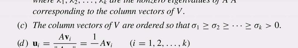
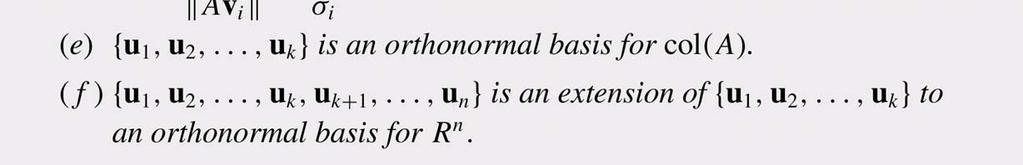
127 8.6. Singular Value Decomposition Singular Value Decomposition of Square Matrices Now consider the set of image vectors This is an orthogonal set, for if i j, then the orthogonality of v i and v j implies that Moreover, from which it follows that Since λ 1 >0 for i=1, 2,, k, it follows from (3) and (4) that is an orthogonal set of k nonzero vectors in the column space of A; and since we know that the column space of A has dimension k (since A has rank k), it follows that (5) is an orthogonal basis for the column space of A.

128 8.6. Singular Value Decomposition Singular Value Decomposition of Square Matrices If we normalize these vectors to obtain an orthonormal basis {u 1, u 2,, u k } for the column space, then Theorem guarantees that we can extend this to an orthonormal basis for R n. Since the first k vectors in this set result from normalizing the vectors in (5), we have which implies that

129 8.6. Singular Value Decomposition Singular Value Decomposition of Square Matrices Now let U be the orthogonal matrix and let Σ be the diagonal matrix It follows from (2) and (4) that Av j =0 for j>k, so which we can rewrite as A=UΣV T using the orthogonality of V.

130 8.6. Singular Value Decomposition Singular Value Decomposition of Square Matrices It is important to keep in mind that the positive entries on the main diagonal of Σ are not eigenvalues of A, but rather square roots of the nonzero eigenvalues of A T A. These numbers are called the singular values of A and are denoted by With this notation, the factorization obtained in the proof of Theorem has the form which is called the singular value decomposition of A (abbreviated SVD of A). The vectors u 1, u 2,, u k are called left singular vectors of A and v 1, v 2,, v k are called right singular vectors of A.

131 8.6. Singular Value Decomposition Singular Value Decomposition of Square Matrices

132 8.6. Singular Value Decomposition Singular Value Decomposition of Square Matrices Example 1 Find the singular value decomposition of the matrix The first step is to find the eigenvalues of the matrix The characteristic polynomial of A T A is so the eigenvalues of ATA are λ 1 =9 and λ 2 =1, and the singular values of A are

133 8.6. Singular Value Decomposition Singular Value Decomposition of Square Matrices Example 1 Unit eigenvectors of A T A corresponding to the eigenvalues λ 1 =9 and λ 2 =1 are and respectively. Thus, so

134 8.6. Singular Value Decomposition Singular Value Decomposition of Square Matrices Example 1 It now follows that the singular value decomposition of A is

135 8.6. Singular Value Decomposition Singular Value Decomposition of Symmetric Matrices Suppose that A has rank k and that the nonzero eigenvalues of A are ordered so that In the case where A is symmetric we have A T A=A 2, so the eigenvalues of A T A are the squares of the eigenvalues of A. Thus, the nonzero eigenvalues of A T A in nonincreasing order are and the singular values of A in nonincreasing order are This shows that the singular values of a symmetric matrix A are the absolute values of the nonzero eigenvalues of A; and it also shows that if A is a symmetric matrix with nonnegative eigenvalues, then the singular values of A are the same as its nonzero eigenvalues.

136 8.6. Singular Value Decomposition Singular Value Decomposition of Nonsquare Matrices If A is an m n matrix, then A T A is an n n symmetric matrix and hence has an eigenvalue decomposition, just as in the case where A is square. Except for appropriate size adjustments to account for the possibility that n>m or n<m, the proof of Theorem carries over without change and yields the following generalization of Theorem

137 8.6. Singular Value Decomposition Singular Value Decomposition of Nonsquare Matrices

138 8.6. Singular Value Decomposition Singular Value Decomposition of Nonsquare Matrices right singular vectors of A singular values of A left singular vectors of A

139 8.6. Singular Value Decomposition Singular Value Decomposition of Nonsquare Matrices Example 4 Find the singular value decomposition of the matrix

140 8.6. Singular Value Decomposition Singular Value Decomposition of Nonsquare Matrices Example 4 A unit vector u 3 that is orthogonal to u 1 and u 2 must be a solution of the homogeneous linear system

141 8.6. Singular Value Decomposition Singular Value Decomposition of Nonsquare Matrices Example 4 Thus, the singular value decomposition of A is

142 8.6. Singular Value Decomposition Singular Value Decomposition of Nonsquare Matrices

143 8.6. Singular Value Decomposition Reduced Singular Value Decomposition The products that involve zero blocks as factors drop out, leaving which is called a reduced singular value decomposition of A U 1 : m k, Σ 1 : k k, and V 1 : k n which is called a reduced singular value expansion of A

144 8.6. Singular Value Decomposition Data Compression and Image Processing If the matrix A has size m n, then one might store each of its mn entries individually. An alternative procedure is to compute the reduced singular value decomposition in which σ 1 σ 2 σ k, and store the σ s, the u s and the v s. When needed, the matrix A can be reconstructed from (17). Since each u j has m entries and each v j has n entries, this method requires storage space for numbers.

145 8.6. Singular Value Decomposition Data Compression and Image Processing It is called the rank r approximation of A. This matrix requires storage space for only numbers, compared to mn numbers required for entry-by-entry storage of A. For example, the rank 100 approximation of a matrix A requires storage for only numbers, compared to the 1,000,000 numbers required for entry-by-entry storage of A a compression of almost 80%. rank 4 rank 10 rank 20 rank 50 rank 128

146 8.6. Singular Value Decomposition Singular Value Decomposition from The Transformation Point of View If A is an m n matrix and T A : R n R m is multiplication by A, then the matrix in (12) is the matrix for T A with respect to the bases {v 1, v 2,, v n } and {u 1, u 2,, u m } for R n and R m, respectively.

147 8.6. Singular Value Decomposition Singular Value Decomposition from The Transformation Point of View Thus, when vectors are expressed in terms of these bases, we see that the effect of multiplying a vector by A is to scale the first k coordinates of the vector by the factor σ 1, σ 2,, σ k, map the rest of the coordinates to zero, and possibly to discard coordinates or append zeros, if needed, to account for a decrease or increase in dimension. This idea is illustrated in Figure for a 2 3 matrix A of rank 2.

148 8.6. Singular Value Decomposition Singular Value Decomposition from The Transformation Point of View Since row(a) =null(a), it follows from Theorem that every vector x in R n can be expressed uniquely as where x row(a) is the orthogonal projection of x on the row space of A and x null(a) is its orthogonal projection on the null space of A. Since Ax null(a) =0, it follows that

149 8.6. Singular Value Decomposition Singular Value Decomposition from The Transformation Point of View This tells us three things: 1. The image of any vector in R n under multiplication by A is the same as the image of the orthogonal projection of that vector on row(a). 2. The range of the transformation T A, namely col(a), is the image of row(a). 3. T A maps distinct vectors in row(a) into distinct vectors in R m. Thus, even though T A may not be one-to-one when considered as a transformation with domain R n, it is one-to-one if its domain is restricted to row(a). REMARK hiding inside of every nonzero matrix transformation T A there is a one-to-one matrix transformation that maps the row space of A onto the column space of A. Moreover, that hidden transformation is represented by the reduced singular value decomposition of A with respect to appropriate bases.

150 8.7. The Pseudoinverse The Pseudoinverse If A is an invertible n n matrix with reduced singular value decomposition then U 1, Σ 1, V 1 are all n n invertible matrices, so the orthogonality of U 1 and V 1 implies that (1) If A is not square or if it is square but not invertible, then this formula does not apply. As the matrix Σ 1 is always invertible, the right side of (1) is defined for every matrix A. If A is nonzero m n matrix, then we call the n m matrix the pseudoinverse of A. (2)

151 8.7. The Pseudoinverse The Pseudoinverse Since A has full column rank, the matrix A T A is invertible (Theorem ) and V 1 is an n n orthogonal matrix. Thus, from which it follows that

152 8.7. The Pseudoinverse The Pseudoinverse Example 1 Find the pseudoinverse of the matrix using the reduced singular value decomposition that was obtained in Example 5 of Section 8.6.

153 8.7. The Pseudoinverse The Pseudoinverse Example 2 A has full column rank so its pseudoinverse can also be computed from Formula (3).

154 8.7. The Pseudoinverse Properties of The Pseudoinverse

155 8.7. The Pseudoinverse Properties of The Pseudoinverse (a) If y is a vector in R m, then it follows from (2) that so A + y must be a linear combination of the column vectors of V 1. Since Theorem states that these vectors are in row(a), it follows that A + y is in row(a).

156 8.7. The Pseudoinverse Properties of The Pseudoinverse (b) Multiplying A + on the right by U 1 yields The result now follows by comparing corresponding column vectors on the two sides of this equation. (c) If y is a vector in null(a T ), then y is orthogonal to each vector in col(a), and, in particular, it is orthogonal to each column vector of U 1 =[u 1, u 2,, u k ]. This implies that U 1T y=0, and hence that

157 8.7. The Pseudoinverse Properties of The Pseudoinverse Example 3 Use the pseudoinverse of to find the standard matrix for the orthogonal projection of R 3 onto the column space of A. The pseudoinverse of A was computed in Example 2. Using that result we see that the orthogonal projection of R 3 onto col(a) is

158 8.7. The Pseudoinverse Pseudoinverse And Least Squares Linear system Ax=b Least square solutions: the exact solution of the normal equation A T Ax=A T b If full column rank, there is a unique least square solution x=(a T A) -1 A T b=a + b If not, there are infinitely many solutions We know that among these least squares solutions there is a unique least square solution in the row space of A (Theorem 7.8.3), and we also know that it is the least squares solution of minimum norm.

159 8.7. The Pseudoinverse Pseudoinverse And Least Squares (1) Let A=U 1 Σ 1 V 1T be a reduced singular value decomposition of A, so Thus, which shows that x=a + b satisfies the normal equation and hence is a least squares solution. (2) x=a + b lies in the row space of A by part (a) of Theorem Thus, it is the least squares solution of minimum norm (Theorem 7.8.3).

160 8.7. The Pseudoinverse Pseudoinverse And Least Squares x + is the least squares solution of minimum norm and is an exact solution of the linear system; that is

161 8.7. The Pseudoinverse Condition Number And Numerical Considerations Ax=b If A is nearly singular, the linear system is said to be ill conditioned. A good measure of how roundoff error will affect the accuracy of a computed solution is given by the ratio of the largest singular value of A to the smallest singular values of A. It is called condition number of A, is denoted by The larger the condition number, the more sensitive the system to small roundoff errors.

162 8.8. Complex Eigenvalues and EigenVectors Vectors in C n modulus (or absolute value) argument polar form complex conjugate The standard operations on real matrices carry over to complex matrices without change, and all of the familiar properties of matrices continue to hold.

163 8.8. Complex Eigenvalues and EigenVectors Algebraic Properties of The Complex Conjugate

164 8.8. Complex Eigenvalues and EigenVectors The Complex Euclidean Inner Product If u and v are column vectors in R n, then their dot product can be expressed as The analogous formulas in C n are

165 8.8. Complex Eigenvalues and EigenVectors The Complex Euclidean Inner Product Example 2

166 8.8. Complex Eigenvalues and EigenVectors The Complex Euclidean Inner Product (c)

167 8.8. Complex Eigenvalues and EigenVectors Vector Space Concepts in C n Except for the use of complex scalars, notions of linear combination, linear independence, subspace, spanning, basis, and dimension carry over without change to C n, as do most of the theorems we have given in this text about them.

168 8.8. Complex Eigenvalues and EigenVectors Complex Eigenvalues of Real Matrices Acting on Vectors in C n complex eigenvalue, complex eigenvector, eigenspace Ax= λx since A has real entries

169 8.8. Complex Eigenvalues and EigenVectors Complex Eigenvalues of Real Matrices Acting on Vectors in C n Example 3 Find the eigenvalues and bases for the eigenspaces of With λ=i, With λ=-i,

170 8.8. Complex Eigenvalues and EigenVectors A Proof That Real Symmetric Matrices Have Real Eigenvalues Suppose that λ is an eigenvalue of A and x is a corresponding eigenvector. where x 0. which shows the numerator is real. Since the denominator is real, λ is real.

171 8.8. Complex Eigenvalues and EigenVectors A Geometric Interpretation of Complex Eigenvalues of Real Matrices Geometrically, this theorem states that multiplication by a matrix of form (19) can be viewed as a rotation through the angle φ followed by a scaling with factor λ.

172 8.8. Complex Eigenvalues and EigenVectors A Geometric Interpretation of Complex Eigenvalues of Real Matrices This theorem shows that every real 2 2 matrix with complex eigenvalues is similar to a matrix form (19).

173 8.8. Complex Eigenvalues and EigenVectors A Geometric Interpretation of Complex Eigenvalues of Real Matrices If we now view P as the transition matrix from the basis B={Re(x), Im(x)} to the standard basis, then (22) tells us that computing a product Ax 0 can be broken down into a three-step process: 1. Map x 0 from standard coordinates into B-coordinates by forming the product P -1 x 0. (22) 2. Rotate and scale the vector P -1 x 0 by forming the product SR φ P -1 x Map the rotated and scaled vector back to standard coordinates to obtain

174 8.8. Complex Eigenvalues and EigenVectors A Geometric Interpretation of Complex Eigenvalues of Real Matrices Example 5 A has eigenvalues and that corresponding eigenvectors are If we take and in (21) and use the fact that λ =1, then

175 8.8. Complex Eigenvalues and EigenVectors A Geometric Interpretation of Complex Eigenvalues of Real Matrices Example 5 The matrix P in (23) is the transition matrix from the basis to the standard basis, and P -1 is the transition matrix from the standard basis to the basis B. In B-coordinates each successive multiplication by A causes the point P -1 x 0 to advance through an angle, thereby tracing a circular orbit about the origin. However, the basis B is skewed (not orthogonal), so when the points on the circular orbit are transformed back to standard coordinates, the effect is to distort the circular orbit into the elliptical orbit.

176 8.8. Complex Eigenvalues and EigenVectors A Geometric Interpretation of Complex Eigenvalues of Real Matrices Example [x 0 is mapped to B-coordinates] [The point (1,1/2) is rotated through the angle φ] [The point (1/2,1) is mapped to standard coordinates]

177 8.8. Complex Eigenvalues and EigenVectors A Geometric Interpretation of Complex Eigenvalues of Real Matrices Section 6.1, Power Sequences

178 8.9. Hermitian, Unitary, and Normal Matrices Hermitian and Unitary Matrices REMARK Part (b) of Theorem The order in which the transpose and conjugate operations are performed in computing does not matter. In the case where A has real entries we have A * =A T, so, A * is the same as A T for real matrices.

179 8.9. Hermitian, Unitary, and Normal Matrices Hermitian and Unitary Matrices Example 1 Find the conjugate transpose A * of the matrix 1 i i 0 A 2 3 2i i and hence 1 i i * A i i

180 8.9. Hermitian, Unitary, and Normal Matrices Hermitian and Unitary Matrices Formula (9) of Section 8.8 v * u

181 8.9. Hermitian, Unitary, and Normal Matrices Hermitian and Unitary Matrices The unitary matrices are complex generalizations of the real orthogonal matrices and Hermitian matrices are complex generalization of the real symmetric matrices.

182 8.9. Hermitian, Unitary, and Normal Matrices Hermitian and Unitary Matrices Example 2 1 i 1 i A i 5 2 i 1 i 2 i 3 1 i 1 i i 2 i 3 * T A A i i A Thus, A is Hermitian.

183 8.9. Hermitian, Unitary, and Normal Matrices Hermitian and Unitary Matrices The fact that real symmetric matrices have real eigenvalues is a special case of the more general result about Hermitian matrices. Let v 1 and v 2 be eigenvectors corresponding to distinct eigenvalues λ 1 and λ 2. A=A *, This implies that (λ 1 - λ 2 )( )= 0 and hence that =0 (since λ 1 λ 2 ).

184 8.9. Hermitian, Unitary, and Normal Matrices Hermitian and Unitary Matrices Example 3 Confirm that the Hermitian matrix has real eigenvalues and that eigenvectors from different eigenspaces are orthogonal. 1: x1 1 i t x 2 1 4: x t x i v 1 1 i 1 v i 1

185 8.9. Hermitian, Unitary, and Normal Matrices Hermitian and Unitary Matrices

186 8.9. Hermitian, Unitary, and Normal Matrices Hermitian and Unitary Matrices Example 4 Use Theorem show that is unitary, and then find A -1. r 1 1 i 1 1 i r 1 1 i 1 1 i Since we now know that A is unitary, if follows that

187 8.9. Hermitian, Unitary, and Normal Matrices Unitary Diagonalizability Since unitary matrices are the complex analogs of the real orthogonal matrices, the following definition is a natural generalization of the idea of orthogonal diagonalizability for real matrices.

188 8.9. Hermitian, Unitary, and Normal Matrices Unitary Diagonalizability Recall that a real symmetric n n matrix A has an orthonormal set of n eigenvectors and is orthogonally diagonalized by any n n matrix whose column vectors are an orthonormal set of eigenvectors of A. 1. Find a basis for each eigenspace of A. 2. Apply the Gram-Schmidt process to each of these bases to obtain orthonormal bases for the eigenspaces. 3. Form the matrix P whose column vectors are the basis vectors obtained in the last step. This will be a unitary matrix (Theorem 8.9.6) and will unitarily diagonalize A.

189 8.9. Hermitian, Unitary, and Normal Matrices Unitary Diagonalizability Example 5 Find a matrix P that unitarily diagonalizes the Hermitian matrix In Example 3, 1: 1 i v1 1 4: v i 1 Since each eigenspace has only one basis vector, the Gram-Schmidt process is simply a matter of normalizing these basis vectors.

190 8.9. Hermitian, Unitary, and Normal Matrices Skew-Hermitian Matrices A square matrix with complex entries is skew-hermitian if A skew-hermitian matrix must have zero or pure imaginary numbers on the main diagonal, and the complex conjugates of entries that are symmetrically positioned about the main diagonal must be negative of one another.

191 8.9. Hermitian, Unitary, and Normal Matrices Normal Matrices Real symmetric matrices Hermitian matrices O Orthogonally diagonalizable Unitarily diagonalizable It can be proved that a square complex matrix A is unitarily diagonalizable if and only if Matrices with this property are said to normal. Normal matrices include the Hermitian, skew-hermitian, and unitary matrices in the complex case and the symmetric, skew-symmetric, and orthogonal matrices in the real case.

192 8.9. Hermitian, Unitary, and Normal Matrices A Comparison of Eigenvalues

193 8.10. Systems of Differential Equations Terminology general solution initial condition initial value problem Example 1 Solve the initial value problem

194 8.10. Systems of Differential Equations Linear Systems of Differential Equations y =Ay (7) homogeneous first-order linear system A: coefficient matrix Observe that y=0 is always a solution of (7). This is called the zero solution or the trivial solution.

195 8.10. Systems of Differential Equations Linear Systems of Differential Equations Example 2

196 8.10. Systems of Differential Equations Fundamental Solutions Every linear combination of solutions of y =Ay is also a solution. Closed under addition and scalar multiplication solution space

197 8.10. Systems of Differential Equations Fundamental Solutions We call S a fundamental set of solutions of the system, and we call a general solution of the system.

198 8.10. Systems of Differential Equations Fundamental Solutions Example 3 Find the fundamental set of solutions. In Example 2, A general solution A fundamental set of solutions

199 8.10. Systems of Differential Equations Solutions Using Eigenvalues and Eigenvectors y=ce at (17) vector x corresponds to coefficient c which shows that if there is a solution of the form (17), then λ must be an eigenvalue of A and x must be a corresponding eigenvector.

200 8.10. Systems of Differential Equations Solutions Using Eigenvalues and Eigenvectors Example 4 Use Theorem to find a general solution of the system 2: x : x1 1 y 1 e 2t 1 1 y 2 1 3t 4 e 1

201 8.10. Systems of Differential Equations Solutions Using Eigenvalues and Eigenvectors Example 4 so a general solution of the system is y ce ce 2t 1 3t y ce ce 2t 3t 2 1 2

202 8.10. Systems of Differential Equations Solutions Using Eigenvalues and Eigenvectors If we assume that Setting t=0, we obtain As x 1, x 2,, x k are linearly independent, so we must have which proves that y 1, y 2,, y k are linearly independent.

203 8.10. Systems of Differential Equations Solutions Using Eigenvalues and Eigenvectors An n n matrix is diagonalizable if and only if it has n linearly independent eigenvectors (Theorem 8.2.6).

204 8.10. Systems of Differential Equations Solutions Using Eigenvalues and Eigenvectors Example 5 Find a general solution of the system In Example 3 and 4 of Section 8.2, we showed the coefficient matrix is diagonalizable by showing that it has an eigenvalue λ=1 with geometric multiplicity 1 and an eigenvalue λ=2 with geometric multiplicity 2. and

205 8.10. Systems of Differential Equations Solutions Using Eigenvalues and Eigenvectors Example 6 At time t=0, tank 1 contains 80 liters of water in which 7kg of salt has been dissolved, and tank 2 contains 80 liters of water in which 10kg of salt has been dissolved. Find the amount of salt in each tank at time t. Now let y 1 (t)=amount of salt in tank 1 at time t y 2 (t)=amount of salt in tank 2 at time t y2 t y1 t y 1 rate in-rate out 8 2 y1 t y2 t y 2 rate in-rate out 2 2