Table of Contents. II. PDE classification II.1. Motivation and Examples. II.2. Classification. II.3. Well-posedness according to Hadamard

Transcription

1 Table of Contents II. PDE classification II.. Motivation and Examples II.2. Classification II.3. Well-posedness according to Hadamard Chapter II (ContentChapterII)

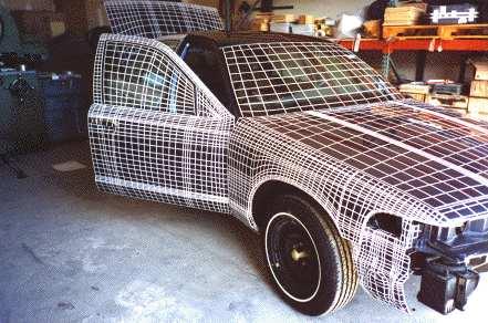
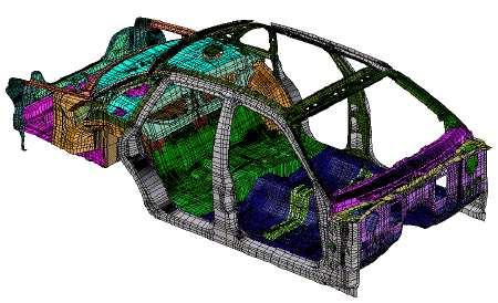
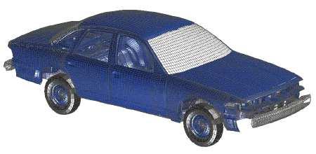
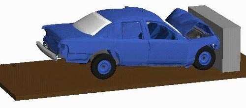
2 Crashtest: Reality Simulation Ford Crown Victoria Removal of components Surface discretization Volume discretization complete model Result of simulation Chapter II (motivation eng) 2

3 Biomechanics msbm/, FE Crash Test Dummy Simulation of injuries after traffic accidents Left: Brain of a rat Right: Simulated deformation of the cortex caused by a traumatic brain injury Chapter II (motivation 2eng) 3

4 Fluid Mechanics: Virtual Wind Tunnel Wing surface Section of the 3D grid Pressure distribution Profile Chapter II (motivation 3eng) 4

5 Earthquake Simulation T. Furumura, Journal of the Earth Simulator 3, 25 Chapter II (motivation 4eng) 5

6 Structural mechanics: Stability of Buildings Chapter II (motivation 5eng) 6

7 Linear Elasticity Determine the deformation field u R d satisfying the Lamé equations divσ(u(x)) = f(x), for x Ω R d and additional boundary conditions on Γ := Ω. f(x) R d : density of volume forces σ(u) R d d : stress tensor σ(u) := λtr(ε(u))id+2µε(u) ε(u) R d d : strain tensor ε(u) := 2 ( u+( u) ) λ,µ R Lamé parameter which can be computed from the elasticity module E and the Poisson s ratio ν of the material. Chapter II (einleitung3eng) 7

8 Linear Elasticity History Cauchy made several contributions to the elasticity theory. For instance, he developed the Cauchy stress tensor of a cube which can completely describe the tension in one point of an elastic body. Augustin Cauchy ( ) Using the Cauchy number, one can draw conclusions about the similarity of elasticity of two bodies. The Cauchy number is the ratio of inertial forces to elastic forces when a body is subject to acoustic oscillations. Chapter II (einleitung39eng) 8

9 Lamé Parameters Plane Strain / Plane Stress In 3 dimensions (d=3): λ = Eν (+ν)( 2ν), µ = E 2(+ν) In 2 dimensions (d=2): Plane Strain λ = Eν (+ν)( 2ν), µ = E 2(+ν) Plane Stress λ = Eν ( ν 2 ), µ = E 2(+ν) The plain stress state is valid for modules with a constant thickness in one direction which is much smaller than the remaining dimensions. Chapter II (einleitung32eng) 9

10 Example Linear Elasticity Plane Strain Profile of a cantilever Force F on the upper side (Neumann data) fixed on the ground (Dirichlet data) Solve for deformation F Chapter II (einleitung33eng)

11 Example: Pressure on a Tube Plane Strain.2 Flow through a tube E = Nm 2, ν =.3, Inner radius r i =.m, Outer radius r a =.2m Pressure on the inside p = 6 Nm 2 Outer side fixed Solve for deformation x 3 Color: abs(u,v) Displacement: (u,v) Chapter II (einleitung34eng)

12 Navier Stokes Equation Navier Stokes equations are a system of second order partial differential equations (PDEs) composed of the momentum theorem and the continuity equation. Their main area of application lies within the fluid mechanics where they are used to describe the flows of liquids and gases. We want to determine the velocity field u R d, d {2,3}, and the pressure p R, satisfying the system of partial differential equations div(ν u)+ (u )u+ p = f div u = and additional boundary conditions (on Γ := Ω) in Ω R d. f(x) R d,x Ω: Body force ν > : Kinematic viscosity Chapter II (einleitung36eng) 2

13 Navier Stokes equations History Claude Navier ( ) The theorem of momentum for newtonian fluids, e.g. for water, was formulated by Navier and Stokes independent from each other during the 9 th century. Even though the equations were derived by Saint Venant two years before Stokes, the name Navier Stokes equations became established. To this day, there is no proof of the well-posedness of the general 3D Navier Stokes equations. George Stokes (89 93) Chapter II (einleitung38eng) 3

14 Navier Stokes equations Example Simulation of a turbulent flow using the Navier Stokes equations. The flow is depicted at the initial and the final stage of the simulation. Chapter II (einleitung37eng) 4

15 Classification A linear second order differential operator with invertible coefficient matrix A(x) L = n i,j= 2 a ij (x) + x i x j n i= b i (x) x i +c(x), A(x) := (a ij (x)) i,j n. is elliptic in x: All n eigenvalues of have the same sign. is parabolic in x: One eigenvalue equals. All other n eigenvalues have the same sign. Additionally, rank(a(x), b(x)) = n holds, with b(x) = (b (x),...,b n (x)) T. is hyperbolic in x: n eigenvalues have the same sign, the other eigenvalue has the opposite sign. The linear, second order PDE ist elliptic/parabolic/hyperbolic on Ω R n, (Ω open), if it is elliptic/parabolic/hyperbolic for all x Ω. Note that x i can be both a spatial and a temporal coordinate, i.e. n = 4 for a 3d and time-dependent problem. Chapter II (einleitung2eng) 5

16 Elliptic partial differential equations Prototype: Laplace operator = d i= 2 x 2 i, A =... Additionally, boundary data on the boundary Γ := Ω of the domain Ω R d need to be imposed:. Dirichlet boundary conditions: u = f in Ω, u = g on Γ 2. Neumann boundary conditions: u = f in Ω, 3. Robin boundary conditions: u = f in Ω, u n = p on Γ u +u = r on Γ n Chapter II (einleitung3eng) 6

17 Elliptic partial differential equations Dirichlet boundary conditions Dirichlet boundary value problem: u= f in Ω u= g on Γ := Ω Ω unit square (,) (,) f(x,y) = 2π 2 sin(2πx)sin(4πy) g(x,y) = exact solution u(x, y) = sin(2πx) sin(4πy) Chapter II (einleitung5eng) 7

18 Dirichlet boundary conditions - example Laplace operator Color: u Height: u Exact solution u(x, y) = sin(2πx) sin(4πy) of the dirichlet boundary value problem Chapter II (einleitung6eng) 8

19 Elliptic partial differential equations Neumann boundary conditions Neumann boundary value problem: Ω unit square (,) (,) u= f in Ω u = g on Γ := Ω n f(x,y) = ( 2x)y 2 (2y 3)+( 2y)x 2 (2x 3) g(x,y) = exact solution u(x,y) = 6 x2 (2x 3)y 2 (2y 3) Chapter II (einleitung8eng) 9

20 Neumann boundary conditions - example Compatibility condition Ω f dx = Ω gds Chapter II (einleitung9eng) 2

21 Elliptic partial differential equations Mixed boundary conditions Example u = in Ω u = on n on 2 on u = 3 on 4 on Chapter II (einleitung2eng) 2

22 Mixed boundary conditions - example Chapter II (einleitung2eng) 22

23 Elliptic partial differential equations Robin boundary conditions Robin boundary value problem: u n Ω unit square (,) (,) f(x,y) = g(x, y) = sin(2πx) cos(4πy) u= f in Ω +u= g on Γ := Ω Chapter II (einleitung22eng) 23

24 Robin boundary conditions - example Chapter II (einleitung23eng) 24

25 Parabolic differential equations Prototype: Heat equation L = t, A =... To obtain a solution u(t,x) for t t and x Ω R d, in addition to the boundary conditions, an initial condition is required: t u u =f for x Ω, t t, e.g. Dirichlet BC: u(t,x) = g(t) for x Γ D, t t, or Neumann BC: u n (t,x) = p(t) for x Γ N, t t, u(t,x) :=u (x) for x Ω Chapter II (einleitung4eng) 25

26 Parabolic differential equation Prototype: Heat transfer equation example t u u = f for x Ω, t t = Ω square (,) (,) f = u = on Ω initial condition u(t,x) = u (x) = { if x B.4 () else Chapter II (einleitung24eng) 26

27 Heat transfer equation - example t = t = t = t = The parabolic operator describes a diffusion process and yields a smooth solution. Local numerical oscillations are also smoothed out Chapter II (einleitung25eng) 27

28 Hyperbolic differential equations Prototype: Wave equation L = 2 t 2, A =... To obtain a solution u(t,x) for t t and x Ω R d, boundary conditions as well as initial conditions need to be imposed: Boundary conditions: Γ := Ω = Γ D Γ N with Γ N Γ D = u = g on Γ D, u n = p on Γ N for t t, Initial conditions: u(t,x) = u (x) and t u(t,x) = u (x) for x Ω. Chapter II (einleitung5eng) 28

29 Hyperbolic differential equations Prototype: Wave equation tt u u = for x Ω, t t = Ω square (,) (,) u = on the left and right boundary u n = on the upper and lower boundary Initial conditions u(t,x) = u (x) = arctan(cos( π 2 x )) t u (x) = u (x) = 3sin(πx)exp(sin( π 2 x 2)) Chapter II (einleitung26eng) 29

30 Wave equation - example t = t = t = t = The hyperbolic operator describes a wave propagation. Unfortunately, local numerical oscillations are propagated as well. Numerical solutions can be tricky and the methods must be robust. Chapter II (einleitung27eng) 3

31 Well-posedness in the sense of Hadamard A problem is called well-posed in the sense of Hadamard iff. the problem has a solution 2. the solution is unique J. Hadamard ( ) 3. the solution depends continuously on the given data (right hand side, initial and/or boundary conditions, ) Chapter II (einleitung43eng) 3