1. Probability density function for speech samples. Gamma. Laplacian. 2. Coding paradigms. =(2X max /2 B ) for a B-bit quantizer Δ Δ Δ Δ Δ

Transcription

1 Digital Speech Processing Lecture 16 Speech Coding Methods Based on Speech Waveform Representations and Speech Models Adaptive and Differential Coding 1

2 Speech Waveform Coding-Summary of Part 1 1. Probability density function for speech samples Gamma Laplacian x σ 1 1 x px ( ) = e p( 0) = σ σ x 1/ 3 x σ 3 x px ( ) = e p( 0) = 8πσ x x x. Coding paradigms uniform -- divide interval from +X X B max to max into intervals of length Δ =(X max / B ) for a B-bit quantizer Δ Δ Δ Δ Δ Δ Δ -X max =4σ x +X max =4σ x

3 Speech Waveform Coding-Summary of Part 1 p(e) xn ˆ( ) = xn ( ) + en ( ) X max SNR = 6B log10 σ x i sensitivity to X / σ ( σ varies a lot!!!) max x i not great use of bits for actual speech densities! X max X max 0log 10 SNR (uniform) (B=8) σx σx x -Δ/ Δ/ over oea3 3:1 range age i Xmax (or equivalently σ x ) varies a lot across sounds, speakers, environments i need dto adapt coder ( Δ ( n))t to time varying σ x or Xmax i key question is how to adapt.. 30 db loss as X max /σ x varies Δ Δ Δ Δ Δ Δ Δ 1/Δ -X 3 max =4σ x +X max =4σ x

4 Speech Waveform Coding-Summary of Part 1 pseudo-logarithmic (constant percentage error) - compress x(n) by pseudo-logarithmic compander - quantize the companded x(n) uniformly - expand the quantized signal [ ] y(n) = F x(n) large xn ( ) xn ( ) log 1 + μ Xmax = X max sign x(n) log( 1+ μ ) X max μ xn ( ) yn ( ) log logμ Xmax [ ] 4 -X max =4σ x +X max =4σ x

5 Speech Waveform Coding-Summary of Part 1 X max X max SNR( db) = 6B log10 [ ln( 1+ μ) ] 10log μσ x μσ x i insensitive to X / σ over a wide range for large μ max x maximum SNR coding match signal quantization intervals to model probability distribution (Gamma, Laplacian) interesting at least theoretically 5

6 Adaptive Quantization linear quantization => SNR depends on σ x being constant t (this is clearly l not the case) instantaneous companding => SNR only weakly dependent on X max /σ x for large μ-law compression ( ) optimum SNR => minimize σ e when σ x is known, nonuniform distribution of quantization levels Quantization dilemma: want to choose quantization step size large enough to accomodate maximum peak-topeak range of x(n); at the same time need to make the quantization step size small so as to minimize the quantization error the non-stationary nature of speech (variability across sounds, speakers, backgrounds) compounds this problem greatly 6

7 Solutions to Quantization Dilemna Adaptive Quantization: Solution 1 -let Δ vary to match the variance of the input signal => Δ(n) Solution - use a variable gain, G(n), followed by a fixed quantizer step size, Δ => keep signal variance of y(n)=g(n)x(n) constant Case 1: Δ(n) proportional to σ x => quantization levels and ranges would be linearly scaled to match σ x => need to reliably estimate σ x Case : G(n) proportional to 1/ σ x to give σ y constant need reliable estimate of σ x for both types of adaptive quantization 7

8 Types of Adaptive Quantization instantaneous-amplitude changes reflect sampleto-sample variations in x[n] => rapid adaptation syllabic-amplitude changes reflect syllable-tosyllable variations in x[n] => slow adaptation feed-forward-adaptive quantizers that estimate σ x from x[n] [ ]itself feedback-adaptive quantizers that adapt the step size, Δ, on the basis of the quantized signal, xˆ[ n ], (or equivalently the codewords, c[n]) 8

9 Feed Forward Adaptation Variable step size assume uniform quantizer with step size Δ[n] x[n] is quantized using Δ[n] => c[n] and Δ[n] need to be transmitted to the decoder if c [n]=c[n] and Δ [n]=δ[n] => no errors in channel, and xˆ [ n[ = xˆ[ n] Don t have x[n] at the decoder to estimate Δ[n] => need to transmit Δ[n]; this is a major drawback of feed forward adaptation 9

10 Feed-Forward Forward Quantizer time varying gain, G[n] => c[n] and G[n] need to be transmitted to the decoder Can t estimate G[n] at the decoder => it has to be transmitted 10

11 Feed Forward Quantizers feed forward systems make estimates of σ x, then make Δ or the quantization levels proportional to σ x, or the gain is inversely proportional to σ x assume σ x σ short-time ti energy [ ] = [ ] [ ] / [ ] where [ ] is a lowpass filter n x m hn m hm hn m= m= 0 E σ [ n] σ x (this can be shown) n 1 consider hn [ ] = α n 1 = 0 otherwise σ [ ] = 1 n ] m= n m 1 n x m α ( 1 α) ( 0< α < 1) σ = ασ + α [ n ] [ n 1 ] + x [ n 1 ]( 1 ) (recursion) this gives Δ [ n] = Δ σ[ n] and G[ n] = G / σ[ n]

12 Slowly Adapting Gain Control α = yn [ ] = Gnxn [ ] [ ] 099. σ [ n] = ασ [ n 1] + x [ n 1](1 α) n 1 n m 1 = x m Gn [ ] = m= = G α 0 σ [ n ] { } yˆ[ n] = Q G[ n] x[ n] Δ [ ](1 α) Δ =Δ [ n] σ 0 [ n] G G[ n] G min Δ Δ[ n] Δ min max max xn ˆ[ ] Q xn [ ] = Δ[ n] { } α =0.99 => brings up level in low amplitude regions => time constant of 100 samples (1.5 msec for 8 khz sampling rate) => syllabic rate 1

13 Rapidly Adapting Gain Control α = 09. yn [ ] = Gnxn [ ] [ ] σ [ n] = ασ [ n 1] + x [ n 1](1 α) n 1 n m 1 = x m Gn [ ] = m= = α G 0 σ [ n ] { } yn ˆ[ ] = Q Gnxn [ ] [ ] Δ Δ =Δ [ ](1 α) [ n] σ 0 [ n] xn ˆ[ ] = Q xn [ ] = Δ[ n] { } G G[ n] G α = 0.9 => system reacts to amplitude variations more min Δ Δ[ n] Δ min max max rapidly => provides better approximation to σ y = constant => time constant of 9 samples (1 msec at 8 khz) for change => instantaneous rate 13

14 Feed Forward Quantizers Δ[n] and G[n] vary slowly compared to x[n] they must be sampled and transmitted as part of the waveform coder parameters rate of sampling depends on the bandwidth of the lowpass filter, h[n] for α = 0.99, the rate is about 13 Hz; for α = 0.9, the rate is about 135 Hz it is reasonable to place limits on the variation of Δ[ n] or G[ n], of the form Gmin G[ n] Gmax Δmin Δ[ n] Δmax for obtaining σ constant over a 40 db range in signal levels => G G max min = Δ Δ y max min = 100 (40dB range) 14

15 Feed Forward Adaptation Gain 1 1 n + σ [ ] = M n x [ m] M m= n Δ[ n] or G[ n] evaluated every M samples used M = 18, 104 samples for estimates adaptive quantizer achieves up to 5.6 db better SNR than non-adaptive quantizers can achieve this SNR with low "idle channel noise" and wide speech dynamic range by suitable choice of Δ and Δ min max feed-forward adaptation gain with B=3 less gain for M=104 than M=18 by 3 db => M=104 is too long an interval 15

16 Feedback Adaptation σ [n] estimated from quantizer output (or the code words) advantage of feedback adaptation is that neither Δ[n] nor G[n] needs to be transmitted to the decoder since they can be derived from the code words disadvantage of feedback adaptation is increased sensitivity to errors in codewords, since such errors affect Δ[n] and G[n] 16

17 Feedback Adaptation σ [ n ] = x ˆ [ m ] h [ n m ] / h [ m ] m= m= 0 ˆ σ [ n] based only on past values of x[ n] two typical windows/filters are n 1 1. hn [ ] = α n 1 = 0 otherwise. hn [ ] = 1/ M 1 n M = 0 otherwise 1 σ [ n] x [ m] 1 = n ˆ M m= n M can use very short window lengths (e.g., 1 db SNR for a B = 3 bit quantizer M = ) to achieve 17

18 Alternative Approach to Adaptation Δ [ n] = P Δ[ n 1]; P = { P, P, P, P } P c [ n 1 ] [ ] Δ[ nsigncn ] [ ] xn ˆ( ) = +Δ[ n] cn [ ] Δ [ n ] only depends ds on Δ[ n 1] and c[ n 1] => only need to transmit codewords also necessary to impose the limits Δmin Δ [n] n Δmax the ratio Δ / Δ controls the dynamic max min range of the quantizer 18

19 Adaptation Gain key issue is how should P vary with c[n-1] if (c[n-1[ [ is either largest positive or largest negative codeword, then quantizer is overloaded and the quantizer step size is too small => P 4 >1 if c[n-1] is either smallest positive or negative codeword, then quantization error is too large => P 1 < 1 need choices for P and P 3 19

20 Adaptation Gain Q = 1+ cn [ 1] B 1 shaded area is variation in range of P values due to different speech sounds or different B values Can see that step size increases (P>1) are more vigorous than step size decreases (P<1) since signal growth needs to be kept within quantizer range to avoid overloads 0

21 Optimal Step Size Multipliers optimal values of P for B=,3,4,5 improvements in SNR 4-7 db improvement over μ-law -4 db improvement over non-adaptive 1 optimum quantizers

22 Quantization of Speech Model Parameters Excitation and vocal tract (linear system) are characterized by sets of parameters which can be estimated from a speech signal by LP or cepstral processing. We can use the set of estimated parameters to synthesize an approximation to the speech signal whose quality depends of a range of factors.

23 Quantization of Speech Model Parameters Quality and data rate of synthesis depends on: the ability of the model to represent speech the ability to reliably and accurately estimate the parameters of the model the ability to quantize the parameters in order to obtain a low data rate digital representation that will yield a high quality reproduction of the speech signal 3

24 Closed-Loop and Open-Loop Speech Coders Closed-looploop used in a feedback loop where the synthetic speech output is compared to the input signal, and the resulting difference used to determine the excitation for the vocal tract model. Open-loop the parameters of the model are estimated directly from the speech signal with no feedback as to the quality of the resulting synthetic ti speech. 4

25 Scalar Quantization Scalar quantization treat each model parameter separately and quantize using a fixed number of bits need to measure (estimate) statistics of each parameter, i.e., mean, variance, minimum/maximum value, pdf, etc. each parameter has a different quantizer with a different number of bits allocated Example of scalar quantization pitch period typically ranges from samples (at 8 khz sampling rate) => need about 18 values (7-bits) uniformly over the range of pitch periods, including value of zero for unvoiced/background amplitude parameter might be quantized with a μ-law quantizer using 4-5 bits per sample using a frame rate of 100 frames/sec, you would need about 700 bps for pitch period and bps for amplitude 5

26 Scalar Quantization 0-th order LPC analysis frame Each PARCOR coefficient transformed to range: π/<sin -1 (k i )<π/ and then quantized with both a 4-bit and a 3-bit uniform quantizer. Total rate of quantized representation of speech about 5000 bps. 6

27 Techniques of Vector Quantization 7

28 Vector Quantization code block of scalars as a vector, rather than individually design an optimal quantization method based on mean-squared distortion metric essential for model-based and hybrid coders 8

29 Vector Quantization 9

30 Waveform Coding Vector Quantizer VQ code pairs of waveform samples, X[n]=(x[n],x[n+1]); [ ], [ ]); (b) Single element codebook with cluster centroid (0-bit codebook) (c) Two element codebook with two cluster centers (1-bit codebook) (d) Four element codebook with four cluster centers (-bit codebook) (e) Eight element codebook with eight cluster centers (3-bit codebook) 30

31 Toy Example of VQ Coding -pole model of the vocal tract => 4 reflection coefficients 4-possible vocal tract shapes => 4 sets of reflection coefficients 1. Scalar Quantization -assume 4 values for each reflection coefficient => -bits x 4 coefficients = 8 bits/frame. Vector Quantization -only 4 possible vectors => -bits to choose which of the 4 vectors to use for each frame (pointer into a codebook) this works because the scalar components of each vector are highly correlated if scalar components are independent => VQ offers no advantage over scalar 31 quantization

32 Elements of a VQ Implementation 1. A large training set of analysis vectors; X={X 1,X,,X L }, L should be much larger than the size of the codebook, M, i.e., times the size of M.. A measure of distance, d ij =d(x i,x j ), between a pair of analysis vectors, both for clustering the training i set as well as for classifying test set vectors into unique codebook entries. 3. A centroid computation procedure and a centroid splitting procedure. 4. A classification procedure for arbitrary analysis vectors that chooses the codebook vector closest in distance to the input vector, providing the codebook index of the resulting nearest codebook vector. 3

33 VQ Implementation 33

34 The VQ Training Set The VQ training set of L 10M vectors should span the anticipated range of: talkers, ranging in age, accent, gender, speaking rate, speaking levels, etc. speaking conditions, range from quiet rooms, to automobiles, to noisy work places transducers and transmission systems, including a range of microphones, telephone handsets, cellphones, speakerphones, etc. speech, including carefully recorded material, conversational speech, telephone queries, etc. 34

35 The VQ Distance Measure The VQ distance measure depends critically on the nature of the analysis vector, X. If X is a log spectral vector, then a possible distance measure would be an L p log spectral distance, of the form: R 1/ p k k p d( Xi, X j) = xi xj k =11 If X is a cepstral vector, then the distance measure might well be a cepstral distance of the form: R k k d ( X i, X j) = ( xi xj ) k = 1 1/ 35

36 Clustering Training Vectors Goal is to cluster the set of L training vectors into a set of M codebook vectors using generalized Lloyd algorithm (also known as the K-means clustering algorithm) with the following steps: 1. Initialization arbitrarily choose M vectors (initially out of the training set of L vectors) as the initial set of codewords in the codebook. Nearest Neighbor Search for each training vector, find the codeword in the current codebook that is closest (in distance) and assign that vector to the corresponding cell 3. Centroid Update update the codeword in each cell to the centroid of all the training vectors assigned to that cell in the current iteration 4. Iteration repeat steps and 3 until the average distance between centroids at successive iterations falls below a preset threshold 36

37 Clustering Training Vectors Voronoi regions and centroids 37

38 Centroid Computation i Assume we have a set of V vectors, C C C C X = { X1, X,..., XV } where all V vectors are assigned to cluster C i The centroid of the set X is defined as the vector Y i that minimizes the average distortion, V 1 C Y = min d( Xi, Y) Y V i = 1 i.e., C. The solution for the centroid is highly dependent C on the choice of distance measure. When both X i and Y are measured in a K-dimensional space with the L norm, the cen troid is the mean of the vector set Y V 1 = X V i = 1 C i i When using an L1 distance measure, the centroid is the median vector of the set of vectors assigned to the given class. 38

39 Vector Classification Procedure i The classification procedure for arbitrary test set vectors is a full search through the codebook to find the "best" (minimum distance) match. i If we denote the codebook vectors of an M -vector codebook as CBi for 1 i M, and we denote the vector to be classified ( and vector quantized) as X, then the index, i, of fthe best codebook entry is: i = arg min d ( X, CB) 1 i M i 39

40 Binary Split Codebook Design 1. Design a 1-vector codebook; the single vector in the codebook is the centroid of the entire set of training vectors. Double the size of the codebook by splitting each current codebook vector, Y m, according to the rule: Y Y + m m = Y (1 + ε ) m = Y (1 ε ) m where m varies from 1 to the size of the current codebook, and epsilon is a splitting parameter (0.01 typically) 3. Use the K-means clustering algorithm to get the best set of centroids for the split codebook 4. Iterate steps and 3 until a codebook of size M is designed. 40

41 Binary Split Algorithm 41

42 VQ Codebook of LPC Vectors 64 vectors in a codebook of spectral shapes 4

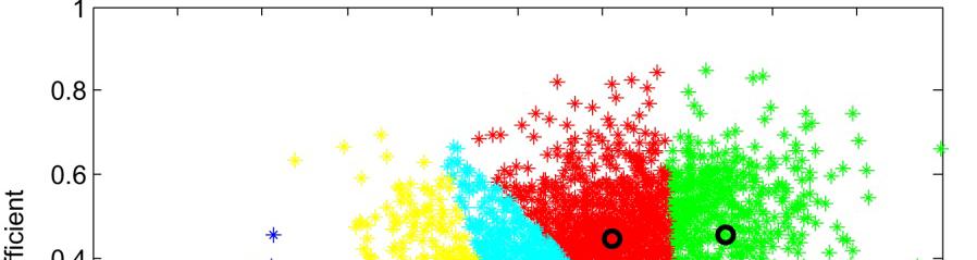
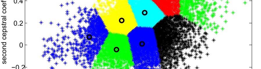
43 VQ Cells 43

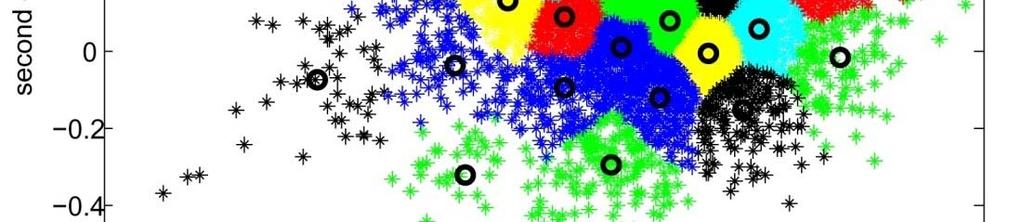
44 VQ Cells 44

45 VQ Coding for Speech distortion in coding computed using a spectral distortion measure related to the difference in log spectra between the original and the codebook vectors 10-bit VQ comparable to 4-bit scalar 45 quantization for these examples

46 Differential Quantization Theory and Practice 46

47 Differential Quantization we have carried instantaneous quantization of x[n] as far as possible time to consider correlations between speech samples separated in time => differential quantization high correlation values => signal does not change rapidly in time => difference between adjacent samples should have lower variance than the signal itself differential quantization can increase SNR at a given bit rate, or lower bit rate for a given SNR 47

48 Example of Difference Signal Prediction error from LPC analysis using p=1 Prediction error is about.5 times smaller than signal 48

49 Differential Quantization Δ xn [ ] + dn [ ] dn ˆ[ ] Q[ ] Encoder cn [ ] xn [ ] xn ˆ[ ] P + (a) Coder dn [ ] = xn [ ] xn [ ] where xn [ ] = unquantized input sample x [ n] = estimate or prediction of x[ n] x [ n] is the output of a predictor system, P, whose input is xˆ [ n], a quantized version of xn [ ] dn [ ] = prediction error signal dn ˆ[ ] = quantized difference (prediction error) signal 49

50 Differential Quantization Δ c'[ n ] ˆ '[ [ ] Decoder + d n x ˆ '[ n ] x '[ n] P (b) Decoder dn [ ] = xn [ ] xn [ ] where xn [ ] = unquantized input sample xn [ ] = estimate or prediction of xn [ ) x [ n] is the output of a predictor system, P, whose input is xˆ [ n], a quantized version of xn [ ] dn [ ] = prediction error signal dn ˆ[ ] = quantized difference (prediction error) signal 50

51 Differential Quantization dn [ ] = xn [ ] xn [ ] dˆ [ n] = d[ n] + e[ n] Δ xn [ ] + dn [ ] dn ˆ[ ] Q[ ] Encoder cn [ ] xn [ ] xn ˆ[ ] P + This part reconstructs the p ( ) = α k Pz z k = 1 quantized signal, xn ˆ[ ] xn ˆ( ) = xn ( ) + dn ˆ ( ) xn ˆ( ) = xn ( ) + en ( ) p xn [ ] = α ˆ k xn [ k] k = 1 k 51

52 Differential Quantization difference signal, d[n], is quantized - not x[n] quantizer can be fixed, or adaptive, uniform or non-uniform quantizer parameters are adjusted to match the variance of d[n] dn ˆ[ ] = dn [ ] + en [ ] en [ ] quantization error xn ˆ[ ] = xn [ ] + dn ˆ[ ] predicted xplus quantized d xn ˆ[ ] = xn [ ] + en [ ] quantized input has same quantization error as the difference signal => if σ d < σ x, error is smaller independent of predictor, P, quantized x[ n] differs from unquantized x[ n ]by en [ ], the quantization error of the difference signal! => good prediction gives lower quantization error than quantizing input directly 5

53 Differential Quantization quantized difference signal is encoded into c(n) for transmission ˆ ˆ ˆ H(z) X ( z) = D ( z) + P( z) X ( z) ˆ 1 X ( z ) = Dˆ ( z ) = H ( z ) Dˆ ( z ) 1 Pz ( ) H( z) = p k = α z k k first reconstruct the quantized difference signal from the decoder codeword, c [n] and the step size Δ next reconstruct the quantized input signal using the same predictor, P, as used in the encoder 53

54 SNR for Differential Quantization the SNR of the differential coding system is SNR where E x [ n] = = E e n x d d σ e σ x [ ] σ e σ σ SNR = = GP SNR σ σ d SNRQ = = σ e Q signal-to-quantizing-noise noise ratio of the quantizer σ x G P = = gain due to differential quantization σ d 54

55 SNR for Differential Quantization Q SNR Q depends on chosen quantizer and can be maximized using all of the previous quantization methods (uniform, non-uniform, optimal) G, hopefully, > 1, is the gain in SNR due to P differential coding want to choose the predictor, P, to maximize GP since σ x is fixed, then we need to minimize σ d, i.e., design the best predictor P 55

56 Predictor for Differential Quantization i consider class of linear predictors, P p xn [ ] = α xn ˆ [ k ] k = 1 k xn [ ] is a linear combination of previous quantized values of xn [ ] the predictor z-transform is p k = 1 ( ) α k Pz = z = 1 Az ( ) -- predictor system function pn [ ] = αk 1 k p = 0 otherwise k with predictor impulse response coefficients (FIR filter) 56

57 Predictor for Differential Quantization i the reconstructed signal is the output, xn ˆ [ ], of a system with system function 1 Xz ˆ ( ) 1 1 Hz ( ) = = = = ˆ ( ) 1 ( ) ( ) 1 α k Dz Pz Az z p k = 1 k where the input to the system is the quantized difference signal, dn ˆ[ ] where p k = 1 dn ˆ [ ] = xn ˆ [ ] α xn ˆ [ k ] p k k = 1 k α xˆ[ n k ] = xn [ ] 57

58 Predictor for Differential Quantization i to solve for optimum predictor, need expression for σ ( ) [ ] [ ] [ ] d = E d n = E x n x n p = E x[ n] α ˆ k x[ n k] k = 1 p p = E x [ n ] α [ ] kx n k αk e [ n k ] k= 1 k= 1 ( xn ˆ[ ] = xn [ ] + en [ ]) σ d 58

59 Solution for Optimum Predictor want to choose { αj }, 1 j p, to minimize σd => differentiate σd wrt α j, set derivatives to zero, giving p σ d = E xn [ ] αk ( xn [ k] + en [ k] ) ( xn [ j] + en [ j] ) α j k = 1 = 0 1 j p which can be written in the more compact form ( ) E x[ n] x[ n] xˆ[ n j] = E d[ n] xˆ[ n j] = 0, 1 j p the predictor coefficients that minimize σ d are the ones that make the difference signal, dn [ ], be uncorrelated with past values of the predictor input, xn ˆ [ j ], 1 j p 59

60 Solution for Alphas ( [ ] [ ]) ˆ[ ] [ ] ˆ[ ] 0, 1 E x n x n x n j = E d n x n j = j p basic equations of differential coding dn ˆ[ ] = dn [ ] + en [ ] quantization of difference signal xn ˆ[ ] = xn [ ] + en [ ] error same for original signal xn ˆ[ ] = xn [ ] + dn ˆ[ ] feedback loop for signal p xn [ ] = α ˆ k xn [ k ] prediction loop based on quantized input k = 1 p dn ˆ[ ] = xn ˆ[ ] α xn ˆ[ k] direct substitution k = 1 xn ˆ[ j] = xn [ j] + en [ j] p k p [ + ] xn [ ] = α xn ˆ [ k ] = α xn [ k ] + en [ k ] k k= 1 k= 1 k 60

61 Solution for Alphas ( ) ˆ ˆ E x[ n] x[ n] x[ n j] = E d[ n] x[ n j] = 0, 1 j p xn ˆ[ j ] = xn [ j ] + en [ j ] p k k= 1 k= 1 p [ ] xn [ ] = α xn ˆ[ k] = α xn [ k] + en [ k] k [ [ ] [ ]] + [ [ ] [ ]] [ [ ] [ ]] [ [ ] [ ]] E x n x n j E x n e n j E x n x n j E x n e n j p = E α k [ x[ n k] + e[ n k] ] x[ n j ] + k =1 p E αk [ x[ n k] + e[ n k] ] e[ n j] k = 1 p [ [ ] [ ]] α [ [ ] [ ]] = α E x n k x n j + E e n k x n j + k k= 1 k= 1 p p [ [ ] [ ]] + α [ [ ] [ ]] α E xn ken j E en ken j k k= 1 k= 1 p k k 61

62 Solution for Optimum Predictor solution for α k - first expand terms to give [ [ ] [ ]] + [ [ ] [ ]] = α [ [ ] [ ]] E x n j x n E e n j x n E x n j x n k p p k = 1 [ [ ] [ ]] α [ [ ] [ ]] + α E en j xn k + E xn j en k k k= 1 k= 1 p αk k = 1 [ ] + Een [ j] en [ k], 1 j p assume fine quantization so that en [ ] is uncorrelated with xn [ ], and en [ ] is stationary white noise (zero mean), giving [ ] 0 [ ] σ E x[ n j] e[ n k] = n, j, k Een [ j] en [ k] = δ [ j k] e p k k 6

63 Solution for Optimum Predictor we can now simplify solution to form [ ] p k [ ] e [ ] k = 1 φ[ j] = α φ[ j k] + σ δ [ j k], 1 j p where φ[ j] is the autocorrelation of x[ n]. Defining terms φ [ j ] σ ρ[ ] = = α ρ[ ] δ[ ], 1 p e j k j k + j k j p σx k = 1 σx or in matrix form ρ = Cα ρ[] 1 α1 1+ 1/ SNR ρ[] 1 ρ[ p 1] α / ρ[ ] ρ[ ] SNR ρ[ p ] ρ =., α =., C =.. ρ[ ] α p ρ[ 1] ρ[ ] 1+ 1/ p p p SNR 63

64 Solution for Optimum Predictor ρ = Cα ρ[] 1 α1 1+ 1/ SNR ρ[] 1 ρ[ p 1] ρ[ ] α ρ[ 1] 1 1/ ρ[ ] + SNR p ρ =., α =., C =.. ρ[ p] α ρ[ 1[ ρ[ ] 1+ 1/ p p p SNR with matrix solution 1 α = C ρ (defining SNR = σ / σ ) x e 1 where C is a Toeplitz matrix C can be computed via well understood => numerical methods C SNR = σ x σ e SNR α k coefficients c e of the predicto r, which depend d on SNR => bit of a dilemma the problem here is that depends on /, but depends on k 64

65 Solution for Optimum Predictor special case of p = 1, where we can solve directly for α of this first order linear predictor, as 1 ρ[] 1 α 1 = 1 + 1/ SNR can see that α1 < ρ[ 1] < 1 we will look further at this special case later 65

66 Solution for Optimum Predictor in spite of problems in solving for optimum predictor coefficients, we can solve for the prediction gain,, in terms of the α coefficients, as E ( x [ n ] x [ n ] ) ( x [ n ] x [ n ] ) E ( x[ n] x [ n] ) x[ n ] ( ) ( xn xn ) σ = G P j d = E x n x n x n x n = E x[ n] x[ n] x [ n] where the term [ ] [ ] is the prediction error; we can show that the second dterm in the expression above is zero, i.e., the prediction error is uncorrelated with the prediction value; thus σ = ( [ ] d E x n x[ n] ) x[ n] = [ ] p E x n E αk ( xn [ k] + en [ k]) xn [ ]) k = 1 assuming uncorrelated signal and noise, we get p p σd = σx αkφ[ k] = σx 1 αkρ[ k] k= 1 k= 1 1 ( GP ) opt = for optimum values of α p k 1 αk ρ [ k ] k = 1 66

67 First Order Predictor Solution For the case p = 1 we can examine effects of α σ σ The optimum solution is: 1 ( G P ) = opt 1 αρ[] 1 sub-optimum value of 1 on the quantity GP = x / d. σ = σ 1 α ρ [] 1 + α + α σ Giving the sub-optimum result 1 Consider choosing an arbitrary value for α ; then we get d x e 1 = 1 αρ[] 1 + α ( 1 + 1/ SNR) ( G ) = G P arb SNR Where the term α / represents the increase in variance of d [ n ] due to the feedback of the error signal en [ ]. 1 67

68 First Order Predictor Solution ( G ) P arb Can reformulate as α1 1 SNRQ ( GP ) = arb 1 αρ 1 [] 1 + α1 for any value of α1 (including the optimum value). Consider the case of α = ρ( 1) 1 ρ [] 1 1 SNR 1 Q ρ [ 1) ( GP ) = = 1 subopt 1 ρ [] 1 1 ρ [] 1 SNR Q the gain in prediction is a product of the prediction gain without the quantizer, reduced by the loss due to feedback of the error signal. 68

69 First Order Predictor Solution We showed before that the optimum value of α was ρ [ 1] / 1+ 1/ [ SNR] If we neglect the term in 1/SNR (usually very small), then α1 = ρ[ 1] and the gain due to prediction is 1 ( G P ) = opt 1 ρ [] 1 Thus thereisapredictiongainsolongas so as ρ [] 1 0 It is reasonable to assume that for speech, ρ[ 1] > 0. 8, giving ( ) G P opt > 77. (or 4.43 db) 1 69

70 Differential Quantization ^ x[n] d[n] d[n] + + Q - Δ x[n] ~ x[n] ^ P + σ σ σ SNR = = = G p SNR σ σ σ x x d e d e First Order Predictor: ρ[] 1 α 1 = 1+ 1/ SNR 1 ρ [] 1 Gp = 1 1 ρ [] 1 SNRQ 1 1 ρ [] 1 Q p xn [ ] = α ˆ k xn [ k] k = 1 dn [ ] = xn [ ] xn [ ] dn ˆ[ ] = dn [ ] + en [ ] xn ˆ[ ] = xn [ ] + dn ˆ[ ] xn ˆ[ ] = xn [ ] + en [ ] The error, e[n], in quantizing d[n] is the same as the error in representing x[n] Prediction gain dependent on ρ[1], the first correlation coefficient 70

71 Long-Term Spectrum and Correlation Measured with 3-point Hamming window

72 Computed Prediction Gain 7

73 Actual Prediction Gains for Speech variation in gain across 4 speakers can get about 6 db improvement in SNR => 1 extra bit equivalent in quantization but at a price of increased complexity in quantization differential quantization works!! gain in SNR depends on signal correlations fixed predictor cannot be optimum for all speakers and for all speech material 73

74 Delta Modulation Linear and Adaptive 74

75 Delta Modulation simplest form of differential quantization is in delta modulation (DM) sampling rate chosen to be many times the Nyquist rate for the input signal => adjacent samples are highly correlated in the limit as T 0, we expect φ x [1] σ as T 0 this leads to a high ability to predict x[n] from past samples, with the variance of the prediction error being very low, leading to a high prediction gain => can use simple 1-bit (-level) l) quantizer => >the bit rate for DM systems is just the (high) sampling rate of the signal 75

76 Linear Delta Modulation -level quantizer with fixed step size, Δ, with quantizer form dn ˆ[ ] =Δ ifdn [ ] > 0 ( cn [ ] = 0 ) = Δ if d[ n] < 0 ( c[ n] = 1) using simple first order predictor with optimum prediction gain 1 ( G P ) = opt 1 ρ [1] as ρ[1] 1, (qualitatively ( ) G P opt only since the assumptions under which the equation was derived break down as ρ[1] 1) 76

77 Illustration of DM basic equations of DM are xn ˆ[ ] = α xn ˆ[ 1] + dn ˆ[ ] when α 1 (essentially digital integration or accumulation of increments of ±Δ) d[ n] = x[ n] x ˆ[ n 1] = x[ n] x[ n 1] e[ n 1] dn [ ] is a first backward difference of xn [ ], or an approximation to the derivative of the input how big do we make Δ--at maximum slope of xa () t we need Δ dx () a t max T dt or else the reconstructed signal will lag the actual signal => called 'slope overload' condition--resulting in quantization error called 'slope overload distortion' since xˆ[ n ] can only increase by fixed increments of Δ, fixed DM is called linear DM or LDM slope overload condition granular noise 77

78 DM Granular Noise when xa() t has small slope, Δ determines the peak error => when xa() t = 0, quantizer will be alternating sequence of 0's and 1's, and xn ˆ[ ] will alternate around zero with peak variation of Δ => this condition is called "granular noise" need large step size to handle wide dynamic range need small step size to accurately represent low level signals with LDM we need to worry about dynamic range and amplitude of the difference signal => choose Δ to minimize mean-squared quantization error (a compromise between slope overload and granular noise) 78

79 Performance of DM Systems normalized step size defined as Δ 1/ E ( x[ n] x[ n 1] ) oversampling index defined as F 0 = F S / ( F N ) where FS is the sampling rate of the DM and FN is the Nyquist frequency of the signal the total bit rate of the DM is BR = FS = FN F 0 can see that for given value of F 0, there is an optimum value of Δ optimum SNR increases by 9 db for each doubling of F 0 => this is better than the 6 db obtained by increasing the number of bits/sample by 1 bit curves are very sharp around optimum value of Δ => SNR is very sensitive to input level for SNR=35 db, for F N =3 khz => 00 Kbps rate for toll quality need much higher rates 79

80 Adaptive Delta Mod step size adaptation for DM (from codewords) Δ [ n] = M Δ[ n 1] Δmin Δ[ n] Δmax M is a function of c[ n] and cn [ 1], since cn [ ] depends only on the sign of d[ n] dn [ ] = xn [ ] α xn ˆ[ 1] the sign of dn [ ] can be determined before theactual quantized value dn ˆ[ ] which needs the new value of Δ[ n] for evaluation the algorithm for choosing the step size multiplier is M= P> 1 if cn [ ] = cn [ 1] M = Q< 1 if c[ n] c[ n 1] 80

81 Adaptive DM Performance slope overload condition granular noise slope overload in LDM causes runs of 0 s 0s or1 s 1s granularity causes runs of alternating 0 s and 1 s figure above shows how adaptive DM performs with P=, Q=1/, α=1 during slope overload, step size increases exponentially to follow increase in waveform slope during ggranularity, step size decreases exponentially to Δ min and stays there as long as slope remains small 81

82 ADM Parameter Behavior ADM parameters are P, Q, Δ min and Δ max choose Δ min and Δ max to provide desired dynamic range choose Δ max / Δ min to maintain high SNR over range of input signal levels Δ min should be chosen to minimize idle channel noise PQ should satisfy PQ 1 for stability PQ chosen to be 1 peak of SNR at P=1.5, but for range 1.5<P<, P, the SNR varies only slightly 8

83 Comparison of LDM, ADM and log PCM ADM is 8 db better SNR at 0 Kbps than LDM, and 14 db better SNR at 60 Kbps than LDM ADM gives a 10 db increase in SNR for each doubling of the bit rate; LDM gives about 6 db for bit rate below 40 Kbps, ADM has higher SNR than μ-law PCM; for higher h bit rates log PCM has higher SNR 83

84 Higher Order Prediction in DM first order predictor gave [ ] = α ˆ[ 1] with reconstructed signal satisfying assuming two real poles, we can write H ( ) z as ˆ ( ) 1 ( ) = Xz H z, 0, 1 ˆ 1 1 ( ) = 1 1 < a b Dz az bz < better prediction is achieved using x n xn ( )( ) xn ˆ[ ] = α xn ˆ[ 1] + dn ˆ[ ] with system function Xˆ ( z) 1 H1( z) = = ˆ 1 Dz ( ) 1 α z digital equivalent of a leaky integrator. consider a second order predictor with x [ n] = α xn ˆ[ 1] + α xn ˆ[ ] 1 this "double integration" system with up to 4 db better SNR there are issues of interaction between the adaptive quantizer and the predictor with reconstructed signal xˆ [ n ] = α ˆ ˆ ˆ 1x[ n 1] + αx[ n ] + d [ n ] with system function Xˆ ( z ) 1 H ( z ) = = ˆ 1 Dz ( ) 1 α z α z ( 1 ) 84

85 Differential PCM (DPCM) fixed predictors can give from 4-11 db SNR improvement over direct quantization (PCM) most of the gain occurs with first order predictor prediction up to 4 th or 5 th order helps 85

86 DPCM with Adaptive Quantization quantizer step size proportional to variance at quantizer input can use d[n] or x[n] to control step size get 5 db improvement in SNR over μ-law nonadaptive PCM get 6 db improvement in SNR using differential configuration with fixed prediction => ADPCM is about db SNR better than from a fixed quantizer 86

87 Feedback ADPCM can achieve same improvement in SNR as feed forward system 87

88 DPCM with Adaptive Prediction need adaptive prediction to handle non-stationarity of speech 88

89 DPCM with Adaptive Prediction prediction coefficients assumed to be time-dependent of the form p x [ n] = α [ n] xˆ [ n k] k = 1 k assume speech properties remain fixed over short time intervals choose αk [ n ] to minimize the average s quared prediction error over short intervals the optimum predictor coefficients satisfy the relationships p n αk n k = 1 R [] j = [] n R [ j k], j = 1,,..., p where R [] j is the short-time autocorrelation function of the form n R [] j = x[ m] w[ n m][ x j + m] w[ n m j], 0 j p n m= wn-m [ ] is window positioned at sample nof input update α's every 10-0 msec 89

90 Prediction Gain for DPCM with Adaptive Prediction i E [ ] 10log10 [ ] 10log x n G P = 10 [ ] E d n fixed prediction 10.5 db prediction gain for large p adaptive prediction 14 db gain for large p adaptive prediction more robust to speaker, speech material 90

91 Comparison of Coders 6 db between curves sharp increase in SNR with both fixed prediction and adaptive quantization almost no gain for adapting first order predictor 91