Small Open Economy. Lawrence Christiano. Department of Economics, Northwestern University

Transcription

1 Small Open Economy Lawrence Christiano Department of Economics, Northwestern University

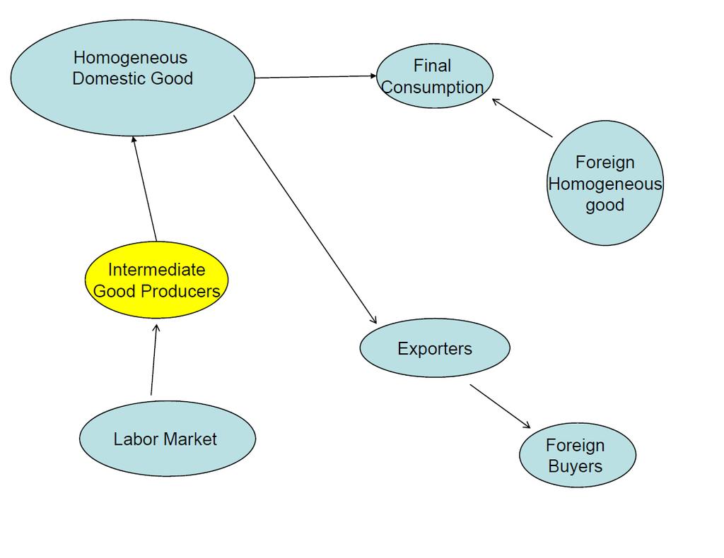
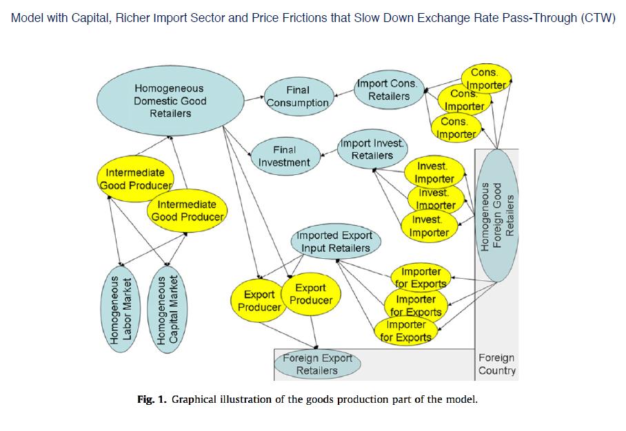
2 Outline Simple Closed Economy Model Extend Model to Open Economy Equilibrium conditions Indicate complications to bring the model to the data. Similar in spirit to Ramses I model Adolfson-Laséen-Lindé-Villan at Swedish Riksbank Brief Discussion of Introducing Financial Frictions Christiano-Trabandt-Walentin (CTW) Model, Ramses II model. Based on Christiano-Motto-Rostagno ( Risk Shocks ) Mihai Copaciu of Romanian Central Bank. Application: will US lift off act like a locomotive to rest of world economy, or will it be a problem (especially for EME s)?

3 Simple Closed Economy Model Results from closed economy model Household preferences: ( E 0 β t { t=0 u (C t ) exp (τ t ) N1+ϕ t 1 + ϕ ), u (C t ) log C t Aggregate resources and household intertemporal optimization: Y t = pt R t A t N t, u c,t = βe t u c,t+1 π t+1 Law of motion of price distortion: ( pt 1 θ (π t ) = (1 ε 1 θ) 1 θ ) ε ε 1 + θπε t pt 1 1 (1)

4 Simple Closed Economy Model Equilibrium conditions associated with price setting: Y t C t + E t π ε 1 t+1 βθf t+1 = F t (2) [ 1 θπ ε 1 t F t 1 θ ] 1 1 ε = K t (3) ε (1 ν) ε 1 = W t Pt by household optimization {}}{ exp (τ t ) N ϕ t 1 Y t u c,t A t C t +E t βθπt+1k ε t+1 = K t (4) note: in simple closed economy model, Y t = C t, but this is not so in open economy. For a derivation in the simple closed economy, see, e.g., Labor_market_handout.pdf

5

6 Extensions to Small Open Economy Outline: the equilibrium conditions of the open economy model system jumps from 6 equations in basic model to 16 equations in 16 variables!

7 Extensions to Small Open Economy: 16 variables rate of depreciation, exports, real foreign assets, terms of trade, real exchange rate {}}{ s t, x t, a f t, p x t, q t price of domestic consumption (now, c is a composite of domestically produced goods & imports) {}}{ p c t price of imports {}}{ p m t consumption price inflation {}}{ π c t reduced form object to (i) achieve technical objective, (ii) adjust UIP implication {}}{ Φ t closed economy variables {}}{ R t, π t, N t, c t, K t, F t, p t

8 Extensions to Small Open Economy- Outline After describing 16 equilibrium conditions: compute the steady state the uncovered interest parity puzzle, and the role of Φ t in addressing the puzzle. summary of the endogenous and exogenous variables of the model, as well as the equations. several computational experiments to illustrate the properties of the model.

9 Modifications to Simple Model to Create Open Economy Unchanged: household preferences production of (domestic) homogeneous good, Y t (= A t pt N t) three Calvo price friction equations Changes: household budget constraint includes opportunity to acquire foreign assets/liabilities. intertemporal Euler equation changed as a reduced form accommodation of evidence on uncovered interest parity. Y t = C t no longer true. introduce exports, imports, balance of payments. exchange rate, S t = domestic currency price of one unit of foreign currency domestic money S t = foreign money

10 Monetary Policy: two approaches Taylor rule ( ) Rt log R = ρ R log +r y log ( Rt 1 R ( yt+1 y ) + (1 ρ R ) E t [r π log ) ] + ε R,t ( π c ) t+1 π c (5) where (could also add exchange rate, real exchange rate and other things): π c ~target consumer price inflation ε R,t ~iid, mean zero monetary policy shock y t ~Y t /A t R t ~ risk free nominal rate of interest ε R,t ~mean zero monetary policy shock.

11 Monetary Policy: two approaches Second approach (Norges Bank, Riksbank) Solve a type of Ramsey problem in which preferences correspond to preferences of monetary policy committee: ( E t β j { 100 [π c t π c t 1 πc t 2 πc t 3 (πc ) 4]) 2 j=0 ( )) 2 yt + λ y (100 log y +λ R (400 [R t R t 1 ]) 2 + λ s (S t S) 2 } straightforward to implement in Dynare. We will stress first approach.

12 Household Budget Constraint Uses of funds less than or equal to sources of funds S t A f t+1 + P t C t + B t+1 B t R t 1 + S t [Φ t 1 R f t 1 Domestic bonds Foreign assets ] A f t + W t N t + transfers and profits t B t ~beginning of period t stock of loans R t ~rate of return on bonds A f t ~beginning-of-period t net stock of foreign assets (liabilities, if negative) held by domestic residents. Φ t Rt f ~rate of return on A f t Φ t ~premium on foreign asset returns

13 Household Intertemporal First Order Conditions: Foreign Assets Optimality of foreign asset choice (verify this by solving Lagrangian representation of household problem) utility cost of 1 unit of foreign currency=s t units of domestic currency, S t /P c t {}}{ u c,t S t P c t units of C t conversion into utility units {}}{ = βe t u c,t+1 quantity of domestic cons. goods purchased from the payoff of 1 unit of foreign currency {}}{ foreign currency payoff next period from one unit of foreign currency today {}}{ S t+1 Rt f Φ t Pt+1 c

14 Household Intertemporal First Order Conditions: Foreign Assets First order condition: Scaling: S t P c t C t = βe t S t+1 R f t Φ t P c t+1 C t+1 1 c t = βe t s t+1 R f t Φ t π c t+1 c t+1 exp ( a t+1 ), s t S t S t 1, c t = C t A t. (6) Technology: a t log (A t ), a t = a t a t 1.

15 Household Intertemporal First Order Conditions: Domestic Assets First order condition: Scaling: 1 R t Pt c = βe t C t Pt+1 c C t+1 1 R t = βe t c t π c t+1 c t+1 exp ( a t+1 ). (7)

16 Final Domestic Consumption Goods Produced by representative, competitive firm using: where C t = [ (1 ω c ) 1 η c ( C d t ) η c 1 η c + ω 1 ηc c ] ηc (Ct m ) η c 1 η c 1 η c Ct d ~ domestic homogeneous output good, price P t Ct m ~ imported good, price Pt m ( St Pt f ) C t ~ final consumption good, Pt c η c ~ elasticity of substitution, domestic and foreign goods.

17 Final Domestic Consumption Goods Profit maximization by representative firm: max P c t C t P m t C m t P t C d t, subject to production function. First order conditions associated with maximization: C m t : P c t ( ) 1 = ω Ct ηc c Ct {}} m { dc t dct m = P m t, C d t : P c t ( ) 1 ηc = (1 ω c ) C t Ct {}}{ d dc t dct d = P t so that the demand functions are: C m t = ω c ( P c t P m t ) ηc Ct, C d t = (1 ω c ) ( ) P c ηc t Ct. P t

18 Price Function Substituting demand functions back into the production function: or C t = [(1 ω c ) 1 η c (C t ( P c t +ω p c t = 1 η c c ( ω c ( P c t P m t P t ) ηc (1 ωc )) η c 1 η c ) ηc Ct ) η c 1 η c ] η c η c 1, [ ] (1 ω c ) + ω c (pt m ) 1 η 1 1 η, c c (8) where p c t Pc t P t, p m t Pm t P t.

19 Real Exchange Rate and Consumption Price Inflation Real Exchange Rate: p m t = Pc t P c t = p c t P m t P t S t P f t P c t, real exchange rate {}}{ q t (9) Consumption good inflation and homogeneous good inflation: π c t Pc t P c t 1 = P tp c t P t 1 p c t 1 = π t [ (1 ω c ) + ω c (p m t ) 1 η c (1 ω c ) + ω c ( p m t 1 ) 1 ηc ] 1 1 η c (10)

20 Exports Foreign demand for domestic goods: ( P x X t = t P f t ) ηf Y f t = (p x t ) η f Y f t, terms of trade {}}{ p x t = Px t P f t Yt f ~ foreign output Pt f ~ foreign currency price of foreign good Pt x ~ foreign currency price of export good Scaling by A t x t = (p x t ) η f y f t (11)

21 Rate of Depreciation, Inflation... Competition: Price of export equals marginal cost: Scaling: Also, S t P x t = P t. 1 = S tpt x = Pc t S t Pt f Pt x P t P t Pt c Pt f = q t pt x pt c (12) q t π = f t s t q t 1 π c, s t S t, π f t t S t 1 Pf t P f t 1 (13)

22 Homogeneous Goods Market Clearing Clearing in domestic homogeneous goods market: output of domestic homogeneous good, Y t = uses of domestic homogeneous goods = goods used in production of final consumption, C t {}}{ exports government {}}{{}}{ Ct d + X t + G t = (1 ω c ) (p c t ) η c C t + X t + G t.

23 Aggregate Employment and Uses of Homogeneous Goods Substituting out in previous expression for Y t : A t p t N t = (1 ω c ) (p c t ) η c C t + X t + G t, or, p t N t = (1 ω c ) (p c t ) η c c t + x t + g t, (14) c t C t A t, x t X t A t, g t G t A t.

24 Balance of Payments equality of international flows relating to trade in goods and in financial assets: acquisition of new net foreign assets, in domestic currency units {}}{ S t A f t+1 + expenses on imports t = receipts from exports t + receipts from existing stock of net foreign assets {}}{ S t R f t 1Φ t 1 A f t

25 Balance of Payments, the Pieces Exports and imports: expenses on imports t = S t P f t ω c ( p c t receipts from exports t = S t P x t X t. p m t ) ηc C t Balance of payments: ) ηc Ct ( p S t A f t+1 + S t Pt f c ω t c pt m = S t Pt x X t + S t Rt 1Φ f t 1 A f t.

26 Balance of Payments, Scaling Scaling by P t A t : S t A f t+1 P t A t + S tp f t P t ω c ( p c t p m t ) ηc ct or, = S tp x t P t x t + S tr f t 1 Φ t 1A f t P t A t, a f t + p m t ω c ( p c t p m t ) ηc ct = pt c q t pt x x t + s trt 1 f Φ t 1at 1 f, (15) π t exp ( a t ) where a f t is scaled, homogeneous goods value of net foreign assets : a f t = S ta f t+1 P t A t.

27 Risk Term ) Φ t = Φ (at f, Rt f, R t, φ t = (16) ( ) ( exp ( φ a at f ā + φ s R t Rt f (R )) ) R f + φ t φ a > 0, small and not important for dynamics φ s > 0, important φ t ~mean zero, iid. Discussion of φ a. φ a > 0 implies (i) if at f > ā, then return on foreign assets low and f ; (ii) if at f < ā, then return on foreign assets high and at f implication: φ a > 0 is a force that drives at f ā in steady state, independent of initial conditions. logic is same as reason why steady state stock of capital in neoclassical growth model is unique, independent of initial conditions. in practice, put in a tiny value of φ a, so that its only effect is to pin down at f in steady state and it does not affect dynamics (see Schmitt-Grohe and Uribe).

28 Risk Term Discussion of φ t : Captures, informally, the possibility that there is a shock to the required return on domestic assets. Discussion of φ s : When φ t > 0, capital outflow shock, people stop liking domestic assets When φ t < 0, safe haven shock, people love domestic assets (e.g., Swiss Franc in recent years). φ s reduced form fix for the model. With φ s = 0, model implies Uncovered Interest Parity (UIP), which does not hold in the data. to better explain this, it is convenient to first solve for the model s steady state.

29 Steady State household intertemporal effi ciency conditions: sr 1 = f β π c exp ( a) (6) R 1 = β π c exp ( a) (7) assumption about foreign households: π f t Pf t P f t 1 (exogenous) R f 1 = β π f exp ( a)

30 Steady State Taylor rule implies: π c = π c, (5). Additional steady state equations: π P t P t 1 = π c (inflation target) (10) p = s = πc π f, R = R f = R/s 1 θπ ε 1 θ ( 1 θ(π) ε 1 1 θ π exp ( a) β ) ε, (no distortion if π c = 1) (1) ε 1 (13) (7) ((6),(7))

31 Steady State, Potentially Iterative Part Rest of the algorithm solves a single non-linear equation in a single unknown, ϕ. Set ϕ = p c q p m = ϕ (9) and p x = 1 ϕ (12) p c = [ ] (1 ω c ) + ω c (p m ) 1 η 1 1 η c c (8) q = ϕ p c

32 Steady State, Potentially Iterative Part... Let g = η g y, ā = η a y. Then, ( ) p 0 = p m c ηc ( ω c c p c p m qp x sr x f ) π exp ( a) 1 η a p N (15) ) 0 = (1 ω c ) (p c ) η c c + x (1 η g Np (14) p F = N c (1 π ε 1 βθ) (2) [ ] 1 1 θπ ε 1 1 ε K = F (3) 1 θ ε 0 = ε 1 (1 ν) N1+ϕ p + (βθπ ε 1) K (4), These five equations involve the five unknowns: c, N, F, K, x. Solve these. Adjust ϕ until (11) is satisfied. In practice, we simply set ϕ = 1 and used (11) to solve for y f.

33 Uncovered Interest Parity Algebra subtract equations (6) and (7): [ R t s t+1 R f ] t Φ t E t c t+1 π c t+1 exp ( a = 0. t+1) totally different object in square brackets and evaluate in steady state: where R t s d t+1 Rt f Φ t c t+1 π c t+1 exp ( a t+1) dr t = cπ c exp ( a) 1 ] [sr f cπ c dφ t + sdrt f + R f ds exp ( a) t+1 R sr f [cπ c exp ( a)] 2 d [ c t+1 π c t+1 exp ( a t+1) ] = 1 { [ ]} ˆR t ˆΦ t + ˆR t f + ŝ t+1 βc ˆx t (x t x) /x = dx t /x.

34 Uncovered Interest Parity, Linearized Representation Then, is, to a first approximation, or, [ R t s t+1 R f ] t Φ t E t c t+1 π c t+1 exp ( a = 0, t+1) [ 1 { [ ]} ] E t ˆR t ˆΦ t + ˆR t f + ŝ t+1 = 0 βc ˆR t = E t ŝ t+1 + ˆR f t + ˆΦ t. Conclude, using dx t x log (x t /x), log Φ = 0 : log R t log R = E t [log s t+1 log (s)] + log R f t log R f + log Φ t or, using log R f = log R log s, definition of s t+1, r t log R t, rt f log Rt f E t log S t+1 log S t = r t r f t + log Φ t

35 Uncovered Interest Parity Under UIP, ˆΦ t = 0 : r t > r f t must be an anticipated depreciation (instantaneous appreciation) of the currency for people to be happy holding the existing stock of net foreign assets Consider regression relation: log S t+1 log S t = β 0 + β 1 (r t r f t ) + u t. Under UIP (and, rational expectations), ˆβ 0 = 0, ˆβ 1 = 1. When ˆΦ t = 0: ˆβ 1 = cov ( log S t+1 log S t, r t rt f ) var ( ) r t rt f = 1 φ s,

36 UIP Puzzle In data, ˆβ 1.75, so UIP rejected (that s the UIP puzzle) Note: because φ s = 1.75 ˆβ 1 = ˆβ 1 = cov ( log S t+1 log S t, r t rt f ) var ( ) r t rt f = 1 φ s, Another way to see UIP puzzle is from VAR impulse responses by Eichenbaum and Evans (QJE, 1992) Data: r t after monetary policy shock log S t+j falls slowly for j = 1, 2, 3,.... UIP theory: r t after monetary policy shock log S t+1 log S t.

37 Intuition Behind UIP Puzzle UIP puzzle: r t and expected appreciation of the currency represents a double-boost to the return on domestic assets. On the face of it, it appears that there is an irresistible profit opportunity. Why doesn t the double-boost to domestic returns launch an avalanche of pressure to buy the domestic currency? In standard models, this pressure produces a greater instantaneous appreciation in the exchange rate, until the familiar UIP overshooting result emerges - the pressure to buy the currency leads to such a large appreciation, that expectations of depreciation emerge. In this way, UIP leads to the counterfactual prediction that a higher r t will be followed (after an instantaneous appreciation) by a period of time during which the currency depreciates.

38 Intuition Behind Resolution of Puzzle Model s resolution of the UIP puzzle: when r t the return required for people to hold domestic bonds rises. This is why the double-boost to domestic returns does not create an appetite to buy large amounts of domestic assets. Possibly this is a reduced form way to capture the notion that increases in r t make the domestic economy more risky. (However, the precise mechanism by which the domestic required return rises - earnings on foreign assets go up - may be diffi cult to interpret. An alternative specification was explored, with risk-premia affecting domestic bonds, but this resulted in indeterminacy problems.)

39 Dynamics 16 equations: price setting, (1),(2),(3),(4); monetary policy rule, (5); household intertemporal Euler equations (6),(7); relative price equations (8),(9),(10),(12),(13); aggregate resource condition, (14); balance of payments, (15); risk term, (16); demand for exports (11). 16 endogenous variables: p c t, p m t, q t, R t, π t, π c t, p x t, N t, p t, a f t, Φ t, s t, x t, c t, K t, F t. exogenous variables: R f t, y f t, φ t, g t, ε R,t, a t, τ t, π f t. for the purpose of numerical calculations, these were modeled as independent scalar AR(1) processes.

40 Extensions to Small Open Economy... the model was solved in the manner described above: - compute the steady state using the formulas described above - log-linearize the 16 equations about steady state - solve the log-linearized system - these calculations were made easy by implementing them in Dynare.

41 Parameter Values Numerical examples: Parameter values: π f = π c = φ a = 0.03 β = /4 θ = 3/4 ϕ = 1 ε = 6 1 ν = ε 1 ε η c = 5 ω c = 0.4 η g = 0.3 η a = 0 η f = 1.5 ρ R = 0.9 r π = 1.5 r y = 0.15

42 Modifying UIP iid shock, 0.01, to ε R,t. φ s = 0 after instantaneous appreciation, positive ε R,t shock followed by depreciation. for higher φ s, shock followed by appreciation. long run appreciation is increasing function of persistence of ρ R.

43 Impact of Modifications to UIP We now consider a monetary policy shock, ε R,t = According to (5), implies a four percentage point (at an annual rate) policy-induced jump in R t. The dynamic effects are displayed in the following figure, for φ s = 0, φ s = 1.75 Note: (i) appreciation smaller, though more drawn out, when φ s is big; (ii) smaller appreciation results in smaller drop in net exports, so less of a drop in demand, so less fall in output and inflation; (iii) smaller drop in net exports results in smaller drop in real foreign assets.

44 Capital Outflow Shock Consider now a domestic economy risk premium shock, a jump in the innovation to φ t equal to With the reduced interest in domestic assets, (i) the currency depreciates, (ii) net exports rise, (iii) hours and output rise, (iv) the upward pressure on costs associated with higher output leads to a rise in prices.

45

46

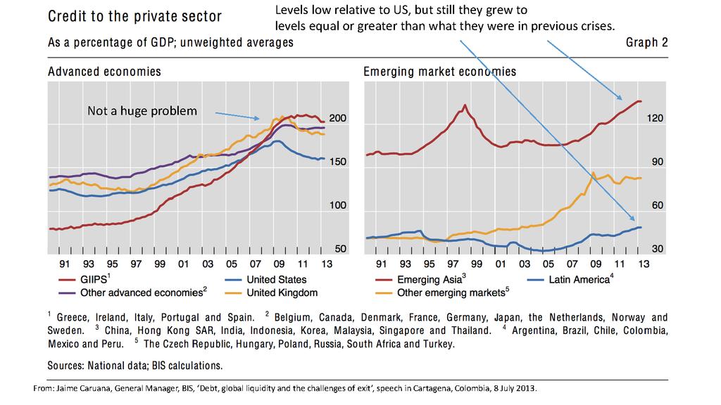
47 Question Confronting Many Emerging Market Economies.. At some point, the Fed will implement its exit strategy and raise US interest rates ( basis points?). In the past, when Fed raised rates sharply (e.g., 1982 Volcker disinflation, 1994 run-up in interest rates), hit the rest of world like a brick: Chilean crisis of 1982, Mexican default of August Mexican crisis of Will the US exit strategy inflict financial crises around the world, especially in emerging market economies? Summer 2013 taper episode makes people worry about this possibility. I ll call the above possibility the BIS scenario.

48 BIS Scenario Low US interest rates since 2008 have encouraged excessive accumulation of debt in the world. This has particularly affected emerging market economies in Asia andlatin America.

49

50 Currency Mismatch Problem May Be Understated.. (Hyun Shin, The Second Phase of Global Liquidity..., November, 2013) Many emerging market borrowers issue dollar-denominated debt through foreign subsidiaries (say in the UK). By the usual definition (based on the residence of the issuer), the bonds are a liability of the UK entity. But, it s the consolidated balance sheet that matters to the emerging market firm. So, the debt issued via a foreign subsidiary could make the emerging market firm vulnerable to currency mismatch problems.

51 Hyun Shin argues: Amount of dollar denominated debt from emerging market firms may be greatly understated. This is suggested by evidence that foreign currency debt by nationality can be much larger than foreign debt by the usual residency definition.

52

53

54

55 Shin conjectures that distinction between external debt according to nationality and residence helps to resolve the taper puzzle: convulsions in emerging markets during taper episode in summer 2013 seem inconsistent with apparently small net external debt position (measured in residence terms) of firms in emerging markets. Less surprising if external debt position is in fact much bigger.

56 BIS Scenario US raises interest rates. Emerging market exchange rates depreciate. Financial health of emerging market firms compromised. They cut back on investment activity....recessions start. Runs on emerging market banks known to be have made loans to now-questionable emerging market non-financial firms. And so on...

57 Locomotive Scenario Previous episodes of US interest rate hikes may be playing too big a role in the pessimistic outlook. The circumstances in which the US raises interest rates may make a difference. In present circumstances, Fed has (credibly, I think) committed to only raise rates until well after the US economy has returned to health. Under these circumstances, interest rate hikes occur when the US is firmly in the position of a locomotive, pulling the rest of the world economy forward in its wake.

58 Which Will it Be: BIS or Locomotive Scenario? Need a model to think about this question. Build in the BIS-type factors that raise concerns about the world economy. Accurately capture the degree of foreign currency indebtedness of financial and nonfinancial firms (i.e., avoid the biases that Hyun Shin is concerned about). Build in the nature of the constraints that cause firms to pull back when their net worth contracts with exchange rate depreciation. Build in the locomotive scenario: Carefully model forward guidance Fed commitment to keep interest rates low even after the US economy has begun to strengthen.

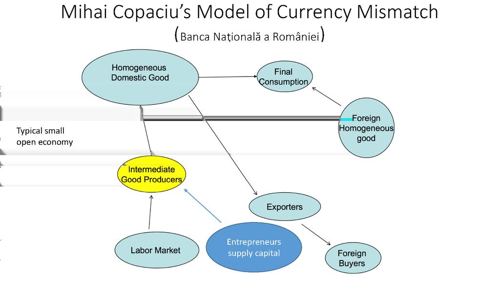
59 A Model Mihai Copaciu (Romanian Central Bank) Constructs small open economy models in which investment is sustained by purchases of entrepreneurs, who earn their revenues in domestic currency units. Entrepreneurs need financing, and the amount of financing they can get is partially a function of their accumulated net worth. Some of the financing is obtained from abroad. When the currency depreciates, entrepreneurs that borrowed abroad make capital losses and their net worth suffers. They are forced to cut back on expenditures, so that investment crashes, bringing down the economy. Same model also contains the usual features that imply an expansion in the US acts as a locomotive on the rest of the world.

60

61

62 DSGE Models Can Play a Useful Role in Discussions about Fed Exit Strategy New Keynesian Open Economy Models can Capture Two Competing Views. Potential for US take-off to: be a locomotive. cause a loss of net worth by foreign firms/financial institutions and force a cut-back in foreign investment ( BIS scenario ).