Data Preprocessing. Jilles Vreeken IRDM 15/ Oct 2015

Transcription

1 Data Preprocessing Jilles Vreeken 22 Oct 2015

2 So, how do you pronounce Jilles Yill-less Vreeken Fray-can Okay, now we can talk.

3 Questions of the day How do we preprocess data before we can extract anything meaningful? How can we convert, normalise, and reduce, Big Data into Mineable Data? 22 Oct 2015 II-1: 3

4 IRDM Chapter 2.1, overview 1. Data type conversion 2. Data normalisation 3. Sampling 4. Dimensionality Reduction You ll find this covered in Aggarwal Chapter Zaki & Meira, Ch. 1, 2.4, 3.5, 6, 7 (Aggarwal, Chapter ) II-1: 4

5 We re here to stay From now on, all lectures will be in HS 002 That is, Tuesday AND Thursday. II-1: 5

6 Homework action speaks louder than words II-1: 6

7 Homework Guidelines Almost every week, we hand out a new homework assignment. You make these individually at home. Homework Timeline: week nn: Homework ii handed out week nn + 1: Hand in results of Homework ii at start of lecture week nn + 2: Tutorial session on Homework ii Questions are to be asked during Tutorial sessions. in exceptional cases of PANIC you may your tutors and kindly ask for an appointment this is beyond their official duty. II-1: 7

8 Homework Guidelines Almost every week, we hand out a new homework assignment. You make these individually at home. Homework Timeline: week nn: Homework ii handed out week nn + 1: Hand as soon in results as of Homework possible ii at start of lecture week nn + 2: Tutorial session on Homework ii Questions are to be asked during Tutorial sessions. Please register for a tutorial group in exceptional cases of PANIC you may your tutors and kindly ask for an appointment this is beyond their official duty. II-1: 8

9 Conversion From one data type to another Ch II-1: 9

10 Data During IRDM we will consider a lot of data. We will refer to our data as DD. We will consider many types. Depending on context DD can be a table, matrix, sequence, etc., with binary, categorical, or real-valued entries. Most algorithms work only for one type of data. How can we convert DD from one type into another? Today we discuss two basic techniques to get us started. II-1: 10

11 Numeric to Categorical - Discretisation How to go from numeric to categorical? by partitioning the domain of numeric attribute dd ii into kk adjacent ranges, and assigning a symbolic label to each. e.g. we partition attribute age into ranges of 10 years: [0,10), [10,20), etc. Standard approaches to choose ranges include Equi-width: choose [aa, bb] such that bb aa is the same for all ranges Equi-log: choose [aa, bb] such that log bb log aa is the same for all Equi-height: choose ranges such each has the same number of records Choosing kk is difficult. Too low, and you introduce spurious associations. Too high, and your method may not be able to find anything. So, be careful; use domain knowledge, just try, or, use more advanced techniques. II-1: 11

12 Categorical to Numeric - Binarisation How to go from categorical to numeric or binary data? by creating a new attribute per categorical attribute-value combination. for each categorical attribute dd with φφ possible values, we create φφ new attributes, and set their values to 0 or 1 accordingly. For example, for attribute colour with domain {rrrrrr, bbbbbbbb, gggggggggg}, we create 3 new attributes, resp. corresponding to cccccccccccc = rrrrrr, cccccccccccc = bbbbbbbb, and cccccccccccc = gggggggggg. Note! If you are not careful, the downstream method does not know what the old attributes are, and will get lost (or, go wild) with the all the correlations that exist between the new attributes. II-1: 12

13 Cleaning Missing Values and Normalisation Ch. 2.3 II-1: 13

14 Missing Values Missing values are common in real-world data in fact, complete data is the rare case values are often unobserved, wrongly observed, or lost Data with missing values needs to be dealt with care some methods are robust to missing values e.g. naïve Bayes classifiers some methods cannot handle missing values (natively) (at all) e.g. support vector machines II-1: 14

15 Handling missing values Two common techniques to handle missing values are ignoring them imputing them In imputation, we replace them with educated guesses either we use high level statistics, e.g. the mean of the variable perhaps stratified over some class e.g. the mean height vs. the mean height of all professors or, we fit a model to the data, and draw values from it e.g. a Bayesian network, a low-rank matrix factorization, etc, matrix completion is often used when lots of values are missing II-1: 15

16 Some problems Imputed values may be wrong! this may have a significant effect on results especially categorical data is hard the effect of imputation is never smooth Ignoring records or variables with missing values may not be possible there may not be any data left Binary data has the problem of distinguishing non-existent and non-observed data did you never see the polar bear living in the Dudweiler forest, or does it not exist? II-1: 16

17 Centering Consider DD of nn observations over mm variables if you want, you can see this as an nn-by-mm matrix DD We say DD is zero centered if mmmmmmmm(ddii) = 0 for each column ddii of DD We can center any dataset by subtracting the mean from each columns II-1: 17

18 Unit variance An attribute dd has unit variance if vvvvvv dd = 1 A dataset DD has unit variance iff ddii var dd ii = 1 We obtain unit variance by dividing every column by its standard deviation. II-1: 18

19 Standardisation Data that is zero centered and has unit variance is called standardised, or the zz-scores many methods (implicitly) assume data is standardised Of course, we may apply non-linear transformations to the data before standardising. for example, by taking a logarithm, or the cubic root we can diminish the importance of LARGE values II-1: 19

20 Why centering? Consider the red data elipse the main dimension of variance is from the origin to the data the second is orthogonal to the first they don t show the variance of the data! If we center the data, however, the directions are correct! II-1: 20

21 When not to center? Centering cannot be applied to all sorts of data It destroys non-negativity e.g. NMF becomes impossible Centered data won t contain integers e.g. no more count or binary data can hurt integratability itemset mining becomes impossible Centering destroys sparsity bad for algorithmic efficiency (we can retain sparsity by only changing non-zero values) II-1: 21

22 Why unit variance? Assume one observation is height in meters, and one observation is weight in grams now weight contains much higher values (for humans, at least) weight has more weight in calculations Division by standard deviation makes all observations equally important most values now fall between -1 and 1 Question to the audience: What s the catch? What s the assumption? II-1: 22

23 What s wrong with unit variance? Dividing by standard deviation is based on the assumption that the values follow a Gaussian distribution often this is plausible: Law of Large Numbers, Central Limit Theorem, etc. Not all data is Gaussian. integer counts (especially over small ranges_ transaction data Not all data distributions have a mean powerlaw distributions II-1: 23

24 Dimensionality Reduction From many to few(er) dimensions Ch II-1: 24

25 Curse of Dimensionality Life gets harder, exponentially harder as dimensionality increases. Not just computationally The data volume grows too fast 100 evenly-spaced points in a unit interval have a max distance of 0.01 to get the same distance for adjacent points in a 10-dimensional unit hypercube we need points that is an increase of factor (!) And, ten dimensions is really not so many II-1: 25

26 Hypercube and Hypersphere A hypercube is a dd-dimensional cube with edge length 2rr, its volume is vvvvvv(hh dd (2rr)) = 2rr dd A Hypersphere is the dd-dimensional ball of radius rr vvvvvv SS 1 rr = 2rr vvvvvv SS 2 rr = ππrr 2 vvvvvv SS 3 rr = 4 3 ππrr3 vvvvvv SS dd rr = KK dd rr dd where KK dd = ππdd/2 Γ dd/2+1 Γ dd = dd 2! for even dd II-1: 26

27 Where is Waldo? (1) Let s say we consider that any two points within the hypersphere are close to each other. The question then is, how many points are close? Or, better, how large is the ball in the box? II-1: 27

28 Hypersphere within a Hypercube Mass is in the corners! Fraction of volume hypersphere has of surrounding hypercube: vvvvvv SS dd rr ππ dd/2 lim = lim dd vvvvvv HH dd 2rr dd 2 dd Γ dd II-1: 28

29 Hypersphere within a Hypercube Mass is in the corners! 2D 3D 4D higher dimensions II-1: 29

30 Where is Waldo? (2) Let s now say we consider any two points outside the sphere, in the same corner of the box, are close to each other. Then, the question is, how many points will be close? Or, better, how cornered is the data? II-1: 30

31 Volume of thin shell of hypersphere SS dd (rr, εε) Mass is in the shell! vvvvvv(ss dd (rr, εε)) = vvvvvv(ss dd (rr)) vvvvvv(ss dd (rr εε)) = KK dd rr dd KK dd rr εε dd Fraction of volume in the shell: vvvvvv SS dd rr,εε vvvvvv SS dd rr = 1 1 εε rr dd vvvvvv SS dd rr, εε lim dd vvvvvv SS dd rr = lim dd 1 1 εε rr dd 1 II-1: 31

32 Back to the Future Dimensionality Reduction II-1: 32

33 Dimensionality Reduction Aim: reduce the number of dimensions by replacing them with new ones the new features should capture the essential part of the data what is considered essential is defined by method you want to use using wrong dimensionality reduction can lead to useless results Usually dimensionality reduction methods work on numerical data for categorical or binary data, feature selection is often more appropriate II-1: 33

34 Feature Subset Selection Data DD may include attributes that are redundant and/or irrelevant to the task at hand. Removing these will improve efficiency and performance. That is, given data DD over attributes AA, we want that subset SS AA of kk attributes such that performance is maximal. Two big problems: 1) how to quantify performance? 2) how to search for good subsets? II-1: 34

35 Searching for Subsets How many subsets of AA are there? 2 AA When do we need to do feature selection? when AA is large oops. Can we efficiently search for the optimal kk-subset? the theoretical answer: depends on your score the practical answer: almost never II-1: 35

36 Scoring Feature Subsets There are two main approaches for scoring feature spaces Wrapper methods optimise for your method directly score each candidate subset by running your method only makes sense when your score is comparable slow, as it needs to run your method for every candidate Filter methods use an external quality measure score each candidate subset using a proxy only makes sense when the proxy optimises your goal can be fast, but may optimise the wrong thing II-1: 36

37 Principle component analysis II-1: 37

38 Principle component analysis The goal of principle component analysis (PCA) is to project the data onto linearly uncorrelated variables in a (possibly) lower-dimensional subspace that preserves as much of the variance of the original data as possible it is also known as Karhunen Lòeve transform or Hotelling transform and goes by many other names In matrix terms, we want to find a column-orthogonal nn-by-rr matrix UU that projects an nn-dimensional data vector xx into an rr-dimensional vector aa = UU TT xx II-1: 38

39 Linear Algebra Recap II-1: 39

40 Vectors A vector is a 1D array of numbers a geometric entity with magnitude and direction The norm of a vector defines its magnitude Euclidean (LL 2 ) norm: xx = xx 2 = nn 2 ii=1 xx 1/2 ii LL pp norm (1 pp ) xx pp = nn ii=1 xx ii pp 1/pp (1.2, 0.8) (2, 0.8) rad (33.69 ) The direction is the angle 40 II-1:

41 Basic operations on vectors A transpose vv TT transposes a row vector into a column vector and vice versa If vv, ww R nn, vv + ww is a vector with vv + ww ii = vv ii + ww ii For vector vv and scalar αα, ααvv ii = ααvv ii A dot product of two vectors vv, ww R nn is vv ww = nn ii=1 a.k.a. scalar product or inner product alternative notation: vv, ww, vv TT ww, vvww TT in Euclidean space vv ww = vv ww cos θθ vv ii ww ii II-1: 41

42 Basic operations on matrices Matrix transpose AA TT has the rows of AA as its columns If AA and BB are nn-by-mm matrices, then AA + BB is an nn-by-mm matrix with AA + BB iiii = mm iiii + nn iiii If AA is nn-by-kk and BB is kk-by-mm, then AABB is an nn-by-mm matrix with the inner dimension (kk) must agree (!) vector outer product vvww TT (for column vectors) is the matrix product of nn-by-1 and 1-by-mm matrices II-1: 42

43 Types of matrices Diagonal nn-by-nn matrix identity matrix II nn is a diagonal nn-by-nn matrix with 1s in diagonal Upper triangular matrix lower triangular is the transpose if diagonal is full of 0s, matrix is strictly triangular Permutation matrix Each row and column has exactly one 1, rest are 0 Symmetric matrix: MM = MM TT II-1: 43

44 Basic concepts Two vectors xx and yy are orthogonal if their inner product xx, yy is 0 vectors are orthonormal if they have unit norm, xx = yy = 1 in Euclidean space, this means that xx yy cos θθ = 0 which happens iff cos θθ = 0 which means xx and yy are perpendicular to each other A square matrix X is orthogonal if its rows and columns are orthonormal an nn-by-mm matrix XX is row-orthogonal if nn < mm and its rows are orthogonal and column-orthogonal if nn > mm and its columns are orthogonal II-1: 44

45 Linear Independency Vector vv R nn is linearly dependent from a set of vectors WW = {wwii R nn ii = 1,, mm} if there exists a set of coefficients ααii such that if vv is not linearly dependent, it is linearly independent that is, vv cannot be expressed as a linear combination of the vectors in WW A set of vectors VV = {vvvv R nn ii = 1,, mm} is linearly independent if vvii is linearly independent from VV {vvii} for all ii II-1: 45

46 Matrix rank The column rank of an nn-by-mm matrix MM is the number of linearly independent columns of MM The row rank is the number of linearly independent rows of MM The Schein rank of MM is the least integer kk such that MM = AAAA for some nn-by-kk matrix AA and kk-by-mm matrix BB equivalently, the least kk such that MM is a sum of kk vector outer products All these ranks are equivalent! II-1: 46

47 The matrix inverse The inverse of a matrix MM is the unique matrix NN for which MMMM = NNNN = II the inverse is denoted by MM 1 MM has an inverse (is invertible) iff MM is square (nn-by-nn) the rank of MM is nn (full rank) Non-square matrices can have left or right inverses MMMM = II or LLLL = II If MM is orthogonal, then (and only then) MM 1 = MM TT that is, MMMM TT = MM TT MM = II II-1: 47

48 Fundamental decompositions A matrix decomposition (or factorization) presents an nn-by- mm matrix AA as a product of two (or more) factor matrices AA = BBBB For approximate decompositions, AA BBBB The decomposition size is the inner dimension of BB and CC number of columns in BB and number of rows in CC for exact decompositions, the size is no less than the rank of the matrix II-1: 48

49 Eigenvalues and eigenvectors If XX is an nn-by-nn matrix and vv is a vector such that XXXX = λλvv for some scalar λλ, then λλ is an eigenvalue of XX vv is an eigenvector of XX associated to λλ That is, eigenvectors are those vectors vv for which XXXX only changes their magnitude, not direction it is possible to exactly reverse the direction the change in magnitude is the eigenvalue If vv is an eigenvector of XX and αα is a scalar, then ααvv is also an eigenvector with the same eigenvalue II-1: 49

50 Properties of eigenvalues Multiple linearly independent eigenvectors can be associated with the same eigenvalue the algebraic multiplicity of the eigenvalue Every nn-by-nn matrix has nn eigenvectors and nn eigenvalues (counting multiplicity) some of these can be complex numbers If a matrix is symmetric, then all its eigenvalues are real Matrix is invertible iff all its eigenvalues are non-zero II-1: 50

51 Eigendecomposition The (real-valued) eigendecomposition of an nn-by-nn matrix XX is XX = QQΛΛQQ 1 ΛΛ is a diagonal matrix with eigenvalues in the diagonal columns of QQ are the eigenvectors associated with the eigenvalues in ΛΛ Matrix XX has to be diagonalizable PPPPPP 1 is a diagonal matrix for some invertible matrix PP Matrix XX has to have nn real eigenvalues (counting multiplicity) II-1: 51

52 Some useful facts Not all matrices have eigendecomposition not all invertible matrices have eigendecomposition not all matrices that have eigendecomposition are invertible if XX is invertible and has eigendecomposition, then XX 1 = QQΛΛ 1 QQ 1 If XX is symmetric and invertible (and real), then XX has eigendecomposition XX = QQΛΛQQ TT II-1: 52

53 Back to PCA II-1: 53

54 Example of 1-D PCA (again) II-1: 54

55 Principle component analysis, again The goal of principle component analysis (PCA) is to project the data onto linearly uncorrelated variables in a (possibly) lower-dimensional subspace that preserves as much of the variance of the original data as possible it is also known as Karhunen Lòeve transform or Hotelling transform and goes by many other names In matrix terms, we want to find a column-orthogonal nn-by-rr matrix UU that projects an nn-dimensional data vector xx into an rr-dimensional vector aa = UU TT xx II-1: 55

56 Deriving PCA: 1-D case (1) We assume our data is standardised. We want to find a unit vector uu that maximises the variance of the projections uu TT xx ii UU. Scalar uu TT xx ii gives the coordinate of xx ii along uu. As our data is centered the mean is 0, projected to uu this has coordinate 0. The variance of the projection is nn σσ 2 = 1 nn uu TT xx ii μμ uu ii=1 nn ΣΣ = 1 n ii xx ii xx ii TT = uu TT ΣΣuu The covariance matrix for centered data II-1: 56

57 Deriving PCA: 1-D case (2) To maximise the variance σσ 2, we maximise JJ uu = uu TT ΣΣuu λλ(uu TT uu 1) where the second term ensures uu is a unit vector Solving the derivative gives ΣΣuu = λλuu uu is an eigenvector and λλ is an eigenvalue further, uu TT ΣΣuu = uu TT λλuu implies that σσ 2 = λλ so, to maximise variance, we need to take the largest eigenvalue Thus, the first principal component uu is the dominant eigenvector of the covariance matrix ΣΣ II-1: 57

58 Example of 1-D PCA II-1: 58

59 Deriving PCA: rr-dimensions The second principal component should be orthogonal to the first one, and maximise variance adding this constraint and doing the derivation shows that the second principal component is the eigenvector associated with the second highest eigenvalue in fact, to find rr principal components we simply take the rr eigenvectors of ΣΣ associated to the rr highest eigenvalues the total variance is the sum of the eigenvalues It also turns out that maximising the variance minimises the mean squared error nn 1 nn xx ii UU TT xxxx ii=1 II-1: 59

60 Computing PCA We have two options. Either we compute the covariance matrix, and its top-kk eigenvectors, or we use singular value decomposition (SVD) because the covariance matrix ΣΣ = XXXX TT and if XX = UUUUVV TT, the columns of UU are the eigenvectors of XXXX TT as computing the covariance matrix can cause numerical stability issues with the eigendecomposition, this approach is preferred II-1: 60

61 SVD: The Definition Theorem. For every AA R nn mm there exists an nn-by-nn orthogonal matrix UU and an mm-by-mm orthogonal matrix V such that UU TT AAAA is an nn-by-mm diagonal matrix ΣΣ with values σσ 1 σσ 2 σσ min nn,mm 0 in its diagonal That is, every AA has decomposition AA = UUΣΣVV TT It is called the singular value decomposition of AA II-1: 61

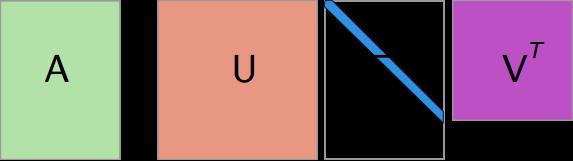
62 SVD in a Picture vv ii are the right singular vectors σσ ii are the singular values uu ii are the left singular vectors II-1: 62

63 SVD, some useful equations AA = UUΣΣVV TT = ii σσ ii uu ii vv ii TT SVD expresses AA as a sum of rank-1 matrices AA 1 = UUΣΣVV TT 1 = VVΣΣ 1 UU TT if AA is invertible, so is its SVD AA TT AAvv ii = σσ ii 2 vv ii (for any AA) AAAA TT uu ii = σσ ii 2 uu ii (for any AA) II-1: 63

64 Truncated SVD The rank of the matrix is the number of its non-zero singular values (write AA = ii σσ ii uu ii vv ii TT ) The truncated SVD takes the first kk columns of UU and VV and the main kk-by-kk submatrix of ΣΣ TT AA kk = UU kk ΣΣ kk VV kk UU kk and VV kk are column-orthogonal II-1: 64

65 Truncated SVD Full Truncated II-1: 65

66 Why is SVD important? It lets us compute various norms It tells about the sensitivity of linear systems It shows the dimensions of the fundamental subspaces It gives optimal solutions to least-square linear systems It gives the least-error rank-k-decomposition Every matrix has one II-1: 66

67 SVD as Low-Rank Approximation Theorem: Let AA be an mm-by-nn matrix with rank rr, and let AA kk = UU kk ΣΣ kk VV kktt, where the kk kk diagonal matrix ΣΣ kk contains the kk largest singular values of AA and the mm kk matrix UU kk and the nn kk matrix VV kk contain the corresponding Eigenvectors from the SVD of A. Among all mm-by-nn matrices CC with rank at most kk AA kk is the matrix that minimizes the Frobenius norm mm nn AA CC 2 FF = ii=1 jj=1 AA iiii CC iiii 2 y Example: mm = 2, nn = 8, kk = 1 projection onto xxx axis minimizes error or maximizes variance in kk-dimensional space x II-1: 67

68 SVD as Low-Rank Approximation Theorem: Let AA be an mm-by-nn matrix with rank rr, and let AA kk = UU kk ΣΣ kk VV kktt, where the kk kk diagonal matrix ΣΣ kk contains the kk largest singular values of AA and the mm kk matrix UU kk and the nn kk matrix VV kk contain the corresponding Eigenvectors from the SVD of A. Among all mm-by-nn matrices CC with rank at most kk AA kk is the matrix that minimizes the Frobenius norm AA CC 2 FF = mm nn ii=1 jj=1 AA iiii CC iiii 2 Example: mm = 2, nn = 8, kk = 1 projection onto xxx axis minimizes error or maximizes variance in kk-dimensional space y II-1: 68 x

69 SVD as Low-Rank Approximation Theorem: Let AA be an mm-by-nn matrix with rank rr, and let AA kk = UU kk ΣΣ kk VV kktt, where the kk kk diagonal matrix ΣΣ kk contains the kk largest singular values of AA and the mm kk matrix UU kk and the nn kk matrix VV kk contain the corresponding Eigenvectors from the SVD of A. Among all mm-by-nn matrices CC with rank at most kk AA kk is the matrix that minimizes the Frobenius norm mm nn AA CC 2 FF = ii=1 jj=1 AA iiii CC iiii 2 Example: mm = 2, nn = 8, kk = 1 projection onto xx axis minimizes error or maximizes variance in kk-dimensional space II-1: 69

70 Problems with PCA and SVD Many characteristics of the input data are lost non-negativity integrality sparsity Also, computation is costly for big matrices approximate methods exist that can do SVD in a single sweep II-1: 70

71 Conclusions Preprocessing your data is crucial Conversion, normalisation, and dealing with missing values Too much data is a problem computational complexity can solved by sampling Too high dimensional data is a problem everything is evenly far from everything feature selections retains important features of the data PCA and SVD reduce dimensionality with global guarantees II-1: 71

72 Thank you! Preprocessing your data is crucial Conversion, normalisation, and dealing with missing values Too much data is a problem computational complexity can solved by sampling Too high dimensional data is a problem everything is evenly far from everything feature selections retains important features of the data PCA and SVD reduce dimensionality with global guarantees II-1: 72