EXPERIMENTAL METHODS SYSTEM QUESTION [70] The governing equations for rocket control are: A dt/dt = Q E = C R
|
|
|
- Jean Moore
- 5 years ago
- Views:
Transcription
1 EXPERIMENTAL METHODS SYSTEM QUESTION [70] The governing equations for rocket control are: X d 2 R/dt 2 + Y dr/dt + Z R = T + M A dt/dt = Q Q = K P E + K I Edτ + K D de/dt E = C R where R is the actual orientation of the rocket in degrees, C is the command orientation, T is a control torque, M is a disturbance torque, Q is the control signal, E is the error signal, X Y Z A are constants and K P K I K D are gains. X=1 Y=2 Z=1 A=10 C o =10 T o =0 Δt=1 Q o =24
2 Sketch an overall block diagram for the rocket. Reduce it down to the two standard GH forms. [5] Determine the rocket transfer functions. Determine the characteristic equation of the rocket. [5] Use the Routh Hurwitz criteria to determine the borderline gain of the system. Is the system stable when K is half the borderline gain? [10] Determine the rocket Ziegler Nichols gains. [10] Develop a NEW from OLD template that would allow the motion of the rocket to be predicted step by step in time. Use the template to get the ZN step response of the rocket 4 steps in time. Write a short m code based on the template. [15] Sketch the Nyquist plot for the case where K is half the borderline gain. Interpret the plot. Estimate the stability margins. Write a short m code for construction of the GH plot. [15] Determine the amplitude and period of the limit cycle generated by an ideal relay controller with DF=10/E o. Is the limit cycle stable? Is the system practically stable? [10]
3 EXPERIMENTAL METHODS SYSTEM QUESTION [70] Equations governing the heading of a boat are: A d 2 R/dt 2 + B dr/dt = T + M X dt/dt + Y T = Z Q Q = K P E + K I Edτ + K D de/dt E = C R where R is the actual heading of the boat in degrees, C is the command heading, T is a control torque, M is a disturbance torque, Q is the control signal, E is the error signal, X Y Z A B are constants and K P K I K D are gains. A=1 B=1 X=1 Y=1 Z=2 C o =10 M o =0 Δt=1 Q o =10
4 Sketch an overall block diagram for the boat. Reduce it down to the two standard GH forms. [5] Determine the boat transfer functions. Determine the characteristic equation of the boat. [5] Use the Routh Hurwitz criteria to determine the borderline gain of the boat. Is the boat stable when K is half the borderline gain? [10] Determine the boat Ziegler Nichols gains. [10] Develop a NEW from OLD template that would allow the motion of the boat to be predicted step by step in time. Use the template to get the ZN step response of the boat 4 steps in time. Write a short m code based on the template. [15] Sketch the Nyquist plot for the case where K is half the borderline gain. Interpret the plot. Estimate the stability margins. Write a short m code for construction of the GH plot. [15] Determine the amplitude and period of the limit cycle generated by an ideal relay controller with DF=10/E o. Is the limit cycle stable? Is the boat practically stable? [10]
5 EXPERIMENTAL METHODS QUIZ #1 SYSTEM QUESTION The equations governing the proportional control of the forward speed of a certain ship are: Plant X dr/dt + Y R = P + D Drive J dp/dt + I P = Q Sensor A dw/dt + B W = R Controller Q = G (C-W) where R is the actual speed of the ship in meters per second, W is the speed in volts as measured by a sensor, C is the command speed in volts, P is the propulsion force, D is a disturbance force, Q is the control signal, J I X Y A B are constants and G is the controller gain. J=1 I=1 X=1 Y=1 A=1 B=1
6 Derive equations for the borderline gain and the borderline period of the system in terms of system parameters. Calculate the borderline gain and period of the system. Use them to determine the Ziegler Nichols Gains of the system. The sensor into the plant and the controller into the drive gives: X (A d 2 W/dt 2 + B dw/dt) + Y (A dw/dt + B W) = P + D J dp/dt + I P = G (C-W) The plant into the drive gives J X (A d 3 W/dt 3 + B d 2 W/dt 2 ) J Y (A d 2 W/dt 2 + B dw/dt) I X (A d 2 W/dt 2 + B dw/dt) + I Y (A dw/dt + B W) - J dd/dt - I D = G (C-W) Manipulation gives JXA d 3 W/dt 3 + (JXB + JYA + IXA) d 2 W/dt 2 + (JYB + IXB + IYA) dw/dt - J dd/dt = G C - (G+IYB) W + I D During borderline stable operation
7 W = W o + W Sin( t) Substitution into the W equation gives - JXA 3 W Cos( t) - (JXB+JYA+IXA) 2 W Sin( t) + (JYB+IXB+IYA) W Cos( t) = G C o - (G+IYB) W o - (G+IYB) W Sin( t) + I D o This equation is of the form i Sin[ t] + j Cos[ t] + k = 0 i = - (JXB+JYA+IXA) 2 + (G+IYB) j = - JXA 3 + (JYB+IXB+IYA) k = - G C o + (G+IYB) W o - I D o Mathematics requires that i=0 j=0 k=0. The j equation gives. The i equation gives G. The k equation gives W o. 2 = (JYB+IXB+IYA) / (JXA) G = (JXB+JYA+IXA) (JYB+IXB+IYA) / (JXA) - IYB W o = (G C o +I D o ) / (G+IYB) The borderline period and gain are: 2 = 3 = 3 T=[2π]/ G = 8
8 Develop a simulation template for PID control of the system. Use this to get the ZN response to a step in command 3 steps in time. Let the time step be 0.5 and let the step height be 5. Let the lower saturation limit on the control signal be 0.0 and the upper limit be Let D be 0. The governing equations can be rewritten as dr/dt = (P + D - Y R) / X dp/dt = (Q - I P) / J dw/dt = (R - B W) / A Q = G P E + G I Edτ + G D de/dt E = (C-W) Application of time stepping gives R NEW = R OLD + t * (P OLD + D OLD - Y R OLD ) / X P NEW = P OLD + t * (Q OLD - I P OLD ) / J W NEW = W OLD + t * (R OLD - B W OLD ) / A Q OLD = G P E OLD + G I E OLD t + G D E OLD / t E OLD = C OLD - W OLD
9 Sketch the overall block diagram for the system. Reduce this down to the standard form for each input. Derive the transfer function for each input.
10 R G = C 1 + GH PID [AS+B] = [XS+Y] [JS+I] [AS+B] + PID
11 R G = D 1 + GH [AS+B] [JS+I] = [XS+Y] [JS+I] [AS+B] + PID
12 Use the ROUTH HURWITZ criteria to derive an equation for the borderline G of the system in terms of system parameters. Calculate the borderline G of the system. Is the system stable when G is half the borderline G? The characteristic equation is [XS+Y] [JS+I] [AS+B] + G = 0 XJA S 3 + (YJA+IXA+BXJ) S 2 + (YJB+YAI+IXB) S + YIB + G = 0 S S S G = 0 This is of the form: a S 3 + b S 2 + c S + d = 0 For borderline operation Routh Hurwitz gives: b*c a*d = 0 Substitution into this gives 3 * 3 = 1 * (1+G) G = 8
13 Use the ROOT LOCUS magnitude and angle concepts to check the borderline G of the system. The GH function is G GH = [XS+Y] [JS+I] [AS+B] G GH = [S+1] [S+1] [S+1] There are 3 identical poles. The angle from each pole to the imaginary axis must add up to 180 o. This implies the angle for each is 60 o. For the intersection of each pole vector with the imaginary axis, geometry gives = 3. The length of each pole vector is 2. The magnitude of GH must be 1. This implies that the borderline gain is G = 2*2*2 = 8.
14
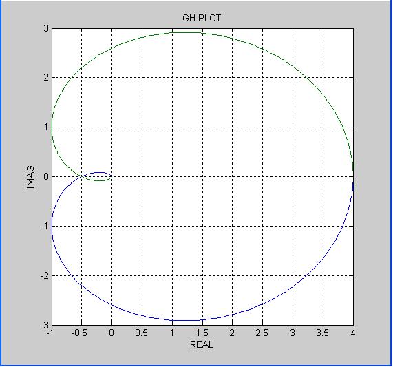
15 Sketch the NYQUIST plot for the case where the gain G is half the borderline G. Estimate the gain and phase margins from the plot. The GH function is G/2 GH = [XS+Y] [JS+I] [AS+B] 4 GH = [S+1] [S+1] [S+1] 4 GH = S S S + 1 Substitution of S=j gives 4 GH = - 3 j j + 1 This shows that as tends to zero this becomes +4 while as tends to infinity it becomes +0j. There is a real axis crossover at -0.5 when is 3 and an imaginary axis crossover at -2.59j when is 1/ 3.
16
17
18 Determine the amplitude and period of the limit cycle generated when the system is controlled by a 5V ideal relay controller. Is the system practically stable with this limit cycle? The describing function for an ideal relay controller is: DF = [4Q o ]/[πe o ] At a limit cycle, this is equal to the borderline proportional gain G. Manipulation gives: G = DF = [4Q o ]/[πe o ] The limit cycle amplitude is: E o = [4Q o ]/[πg] = [4*5]/[π*8] = 0.8 The limit cycle period is: T o = [2π]/ = [2π]/ 3 = 3.6
EXPERIMENTAL METHODS QUIZ #1 SYSTEM QUESTION. The equations governing the proportional control of the forward speed of a certain ship are:
 EXPERIMENTAL METHODS QUIZ #1 SYSTEM QUESTION The equations governing the proportional control of the forward speed of a certain ship are: Plant X dr/dt + Y R = P + D Drive J dp/dt + I P = Q Sensor A dw/dt
ENGINEERING 6951 AUTOMATIC CONTROL ENGINEERING FINAL EXAM FALL 2011 MARKS IN SQUARE [] BRACKETS INSTRUCTIONS NO NOTES OR TEXTS ALLOWED
![ENGINEERING 6951 AUTOMATIC CONTROL ENGINEERING FINAL EXAM FALL 2011 MARKS IN SQUARE [] BRACKETS INSTRUCTIONS NO NOTES OR TEXTS ALLOWED](/thumbs/87/96043431.jpg "ENGINEERING 6951 AUTOMATIC CONTROL ENGINEERING FINAL EXAM FALL 2011 MARKS IN SQUARE [] BRACKETS INSTRUCTIONS NO NOTES OR TEXTS ALLOWED") NAME: JOE CROW ENGINEERING 6951 AUTOMATIC CONTROL ENGINEERING FINAL EXAM FALL 2011 MARKS IN SQUARE [] BRACKETS INSTRUCTIONS NO NOTES OR TEXTS ALLOWED NO CALCULATORS ALLOWED GIVE CONCISE ANSWERS ASK NO
NAME: JOE CROW ENGINEERING 6951 AUTOMATIC CONTROL ENGINEERING FINAL EXAM FALL 2011 MARKS IN SQUARE [] BRACKETS INSTRUCTIONS NO NOTES OR TEXTS ALLOWED NO CALCULATORS ALLOWED GIVE CONCISE ANSWERS ASK NO
ENGINEERING 6951 AUTOMATIC CONTROL ENGINEERING FINAL EXAM FALL 2011 MARKS IN SQUARE [] BRACKETS INSTRUCTIONS NO NOTES OR TEXTS ALLOWED
![ENGINEERING 6951 AUTOMATIC CONTROL ENGINEERING FINAL EXAM FALL 2011 MARKS IN SQUARE [] BRACKETS INSTRUCTIONS NO NOTES OR TEXTS ALLOWED](/thumbs/87/96043394.jpg "ENGINEERING 6951 AUTOMATIC CONTROL ENGINEERING FINAL EXAM FALL 2011 MARKS IN SQUARE [] BRACKETS INSTRUCTIONS NO NOTES OR TEXTS ALLOWED") NAME: JOE CROW ENGINEERING 6951 AUTOMATIC CONTROL ENGINEERING FINAL EXAM FALL 2011 MARKS IN SQUARE [] BRACKETS INSTRUCTIONS NO NOTES OR TEXTS ALLOWED NO CALCULATORS ALLOWED GIVE CONCISE ANSWERS ASK NO
NAME: JOE CROW ENGINEERING 6951 AUTOMATIC CONTROL ENGINEERING FINAL EXAM FALL 2011 MARKS IN SQUARE [] BRACKETS INSTRUCTIONS NO NOTES OR TEXTS ALLOWED NO CALCULATORS ALLOWED GIVE CONCISE ANSWERS ASK NO
NAME: AUTOMATIC CONTROL ENGINEERING ENGINEERING 6951 FINAL EXAMINATION FALL 2014 INSTRUCTIONS
 NAME: AUTOMATIC CONTROL ENGINEERING ENGINEERING 6951 FINAL EXAMINATION FALL 2014 INSTRUCTIONS NO NOTES OR TEXTS ALLOWED NO CALCULATORS ALLOWED NO ELECTRONIC DEVICES ALLOWED ASK NO QUESTIONS THIS EXAM HAS
AUTOMATIC CONTROL ENGINEERING HINCHEY
 AUTOMATIC CONTROL ENGINEERING HINCHEY AUTOMATIC CONTROL ENGINEERING FEEDBACK CONTROL CONCEPT The sketch on the next page shows a typical feedback or error driven control system. What has to be controlled
CONTROL SYSTEM STABILITY. CHARACTERISTIC EQUATION: The overall transfer function for a. where A B X Y are polynomials. Substitution into the TF gives:
 CONTROL SYSTEM STABILITY CHARACTERISTIC EQUATION: The overall transfer function for a feedback control system is: TF = G / [1+GH]. The G and H functions can be put into the form: G(S) = A(S) / B(S) H(S)
7.4 STEP BY STEP PROCEDURE TO DRAW THE ROOT LOCUS DIAGRAM
 ROOT LOCUS TECHNIQUE. Values of on the root loci The value of at any point s on the root loci is determined from the following equation G( s) H( s) Product of lengths of vectors from poles of G( s)h( s)
Video 5.1 Vijay Kumar and Ani Hsieh
 Video 5.1 Vijay Kumar and Ani Hsieh Robo3x-1.1 1 The Purpose of Control Input/Stimulus/ Disturbance System or Plant Output/ Response Understand the Black Box Evaluate the Performance Change the Behavior
Cascade Control of a Continuous Stirred Tank Reactor (CSTR)
") Journal of Applied and Industrial Sciences, 213, 1 (4): 16-23, ISSN: 2328-4595 (PRINT), ISSN: 2328-469 (ONLINE) Research Article Cascade Control of a Continuous Stirred Tank Reactor (CSTR) 16 A. O. Ahmed
Journal of Applied and Industrial Sciences, 213, 1 (4): 16-23, ISSN: 2328-4595 (PRINT), ISSN: 2328-469 (ONLINE) Research Article Cascade Control of a Continuous Stirred Tank Reactor (CSTR) 16 A. O. Ahmed
Course Summary. The course cannot be summarized in one lecture.
 Course Summary Unit 1: Introduction Unit 2: Modeling in the Frequency Domain Unit 3: Time Response Unit 4: Block Diagram Reduction Unit 5: Stability Unit 6: Steady-State Error Unit 7: Root Locus Techniques
Alireza Mousavi Brunel University
 Alireza Mousavi Brunel University 1 » Control Process» Control Systems Design & Analysis 2 Open-Loop Control: Is normally a simple switch on and switch off process, for example a light in a room is switched
Root Locus Methods. The root locus procedure
 Root Locus Methods Design of a position control system using the root locus method Design of a phase lag compensator using the root locus method The root locus procedure To determine the value of the gain
VALLIAMMAI ENGINEERING COLLEGE SRM Nagar, Kattankulathur
 VALLIAMMAI ENGINEERING COLLEGE SRM Nagar, Kattankulathur 603 203. DEPARTMENT OF ELECTRONICS & COMMUNICATION ENGINEERING SUBJECT QUESTION BANK : EC6405 CONTROL SYSTEM ENGINEERING SEM / YEAR: IV / II year
Course roadmap. ME451: Control Systems. What is Root Locus? (Review) Characteristic equation & root locus. Lecture 18 Root locus: Sketch of proofs
 Characteristic equation & root locus. Lecture 18 Root locus: Sketch of proofs") ME451: Control Systems Modeling Course roadmap Analysis Design Lecture 18 Root locus: Sketch of proofs Dr. Jongeun Choi Department of Mechanical Engineering Michigan State University Laplace transform
ME451: Control Systems Modeling Course roadmap Analysis Design Lecture 18 Root locus: Sketch of proofs Dr. Jongeun Choi Department of Mechanical Engineering Michigan State University Laplace transform
a. Closed-loop system; b. equivalent transfer function Then the CLTF () T is s the poles of () T are s from a contribution of a
 T is s the poles of () T are s from a contribution of a") Root Locus Simple definition Locus of points on the s- plane that represents the poles of a system as one or more parameter vary. RL and its relation to poles of a closed loop system RL and its relation
Root Locus Simple definition Locus of points on the s- plane that represents the poles of a system as one or more parameter vary. RL and its relation to poles of a closed loop system RL and its relation
Chapter 6 - Solved Problems
 Chapter 6 - Solved Problems Solved Problem 6.. Contributed by - James Welsh, University of Newcastle, Australia. Find suitable values for the PID parameters using the Z-N tuning strategy for the nominal
Control Systems. University Questions
 University Questions UNIT-1 1. Distinguish between open loop and closed loop control system. Describe two examples for each. (10 Marks), Jan 2009, June 12, Dec 11,July 08, July 2009, Dec 2010 2. Write
Chemical Process Dynamics and Control. Aisha Osman Mohamed Ahmed Department of Chemical Engineering Faculty of Engineering, Red Sea University
 Chemical Process Dynamics and Control Aisha Osman Mohamed Ahmed Department of Chemical Engineering Faculty of Engineering, Red Sea University 1 Chapter 4 System Stability 2 Chapter Objectives End of this
1 An Overview and Brief History of Feedback Control 1. 2 Dynamic Models 23. Contents. Preface. xiii
 Contents 1 An Overview and Brief History of Feedback Control 1 A Perspective on Feedback Control 1 Chapter Overview 2 1.1 A Simple Feedback System 3 1.2 A First Analysis of Feedback 6 1.3 Feedback System
Root Locus. Motivation Sketching Root Locus Examples. School of Mechanical Engineering Purdue University. ME375 Root Locus - 1
 Root Locus Motivation Sketching Root Locus Examples ME375 Root Locus - 1 Servo Table Example DC Motor Position Control The block diagram for position control of the servo table is given by: D 0.09 Position
Table of Laplacetransform
 Appendix Table of Laplacetransform pairs 1(t) f(s) oct), unit impulse at t = 0 a, a constant or step of magnitude a at t = 0 a s t, a ramp function e- at, an exponential function s + a sin wt, a sine fun
Feedback Control of Linear SISO systems. Process Dynamics and Control
 Feedback Control of Linear SISO systems Process Dynamics and Control 1 Open-Loop Process The study of dynamics was limited to open-loop systems Observe process behavior as a result of specific input signals
Compensation 8. f4 that separate these regions of stability and instability. The characteristic S 0 L U T I 0 N S
 S 0 L U T I 0 N S Compensation 8 Note: All references to Figures and Equations whose numbers are not preceded by an "S"refer to the textbook. As suggested in Lecture 8, to perform a Nyquist analysis, we
Contents. PART I METHODS AND CONCEPTS 2. Transfer Function Approach Frequency Domain Representations... 42
 Contents Preface.............................................. xiii 1. Introduction......................................... 1 1.1 Continuous and Discrete Control Systems................. 4 1.2 Open-Loop
Übersetzungshilfe / Translation aid (English) To be returned at the end of the exam!
 To be returned at the end of the exam!") Prüfung Regelungstechnik I (Control Systems I) Prof. Dr. Lino Guzzella 9. 8. 2 Übersetzungshilfe / Translation aid (English) To be returned at the end of the exam! Do not mark up this translation aid -
Prüfung Regelungstechnik I (Control Systems I) Prof. Dr. Lino Guzzella 9. 8. 2 Übersetzungshilfe / Translation aid (English) To be returned at the end of the exam! Do not mark up this translation aid -
6.1 Sketch the z-domain root locus and find the critical gain for the following systems K., the closed-loop characteristic equation is K + z 0.
 6. Sketch the z-domain root locus and find the critical gain for the following systems K (i) Gz () z 4. (ii) Gz K () ( z+ 9. )( z 9. ) (iii) Gz () Kz ( z. )( z ) (iv) Gz () Kz ( + 9. ) ( z. )( z 8. ) (i)
Control Systems. EC / EE / IN. For
 Control Systems For EC / EE / IN By www.thegateacademy.com Syllabus Syllabus for Control Systems Basic Control System Components; Block Diagrammatic Description, Reduction of Block Diagrams. Open Loop
CHAPTER 1 Basic Concepts of Control System. CHAPTER 6 Hydraulic Control System
 CHAPTER 1 Basic Concepts of Control System 1. What is open loop control systems and closed loop control systems? Compare open loop control system with closed loop control system. Write down major advantages
STABILITY OF CLOSED-LOOP CONTOL SYSTEMS
 CHBE320 LECTURE X STABILITY OF CLOSED-LOOP CONTOL SYSTEMS Professor Dae Ryook Yang Spring 2018 Dept. of Chemical and Biological Engineering 10-1 Road Map of the Lecture X Stability of closed-loop control
Linear Control Systems Lecture #3 - Frequency Domain Analysis. Guillaume Drion Academic year
 Linear Control Systems Lecture #3 - Frequency Domain Analysis Guillaume Drion Academic year 2018-2019 1 Goal and Outline Goal: To be able to analyze the stability and robustness of a closed-loop system
Additional Closed-Loop Frequency Response Material (Second edition, Chapter 14)
") Appendix J Additional Closed-Loop Frequency Response Material (Second edition, Chapter 4) APPENDIX CONTENTS J. Closed-Loop Behavior J.2 Bode Stability Criterion J.3 Nyquist Stability Criterion J.4 Gain
Appendix J Additional Closed-Loop Frequency Response Material (Second edition, Chapter 4) APPENDIX CONTENTS J. Closed-Loop Behavior J.2 Bode Stability Criterion J.3 Nyquist Stability Criterion J.4 Gain
(b) A unity feedback system is characterized by the transfer function. Design a suitable compensator to meet the following specifications:
 A unity feedback system is characterized by the transfer function. Design a suitable compensator to meet the following specifications:") 1. (a) The open loop transfer function of a unity feedback control system is given by G(S) = K/S(1+0.1S)(1+S) (i) Determine the value of K so that the resonance peak M r of the system is equal to 1.4.
1. (a) The open loop transfer function of a unity feedback control system is given by G(S) = K/S(1+0.1S)(1+S) (i) Determine the value of K so that the resonance peak M r of the system is equal to 1.4.
Controls Problems for Qualifying Exam - Spring 2014
 Controls Problems for Qualifying Exam - Spring 2014 Problem 1 Consider the system block diagram given in Figure 1. Find the overall transfer function T(s) = C(s)/R(s). Note that this transfer function
Automatic Control III (Reglerteknik III) fall Nonlinear systems, Part 3
 fall Nonlinear systems, Part 3") Automatic Control III (Reglerteknik III) fall 20 4. Nonlinear systems, Part 3 (Chapter 4) Hans Norlander Systems and Control Department of Information Technology Uppsala University OSCILLATIONS AND DESCRIBING
Automatic Control III (Reglerteknik III) fall 20 4. Nonlinear systems, Part 3 (Chapter 4) Hans Norlander Systems and Control Department of Information Technology Uppsala University OSCILLATIONS AND DESCRIBING
CONTROL SYSTEMS ENGINEERING Sixth Edition International Student Version
 CONTROL SYSTEMS ENGINEERING Sixth Edition International Student Version Norman S. Nise California State Polytechnic University, Pomona John Wiley fir Sons, Inc. Contents PREFACE, vii 1. INTRODUCTION, 1
Chapter 7 : Root Locus Technique
 Chapter 7 : Root Locus Technique By Electrical Engineering Department College of Engineering King Saud University 1431-143 7.1. Introduction 7.. Basics on the Root Loci 7.3. Characteristics of the Loci
Lecture 10: Proportional, Integral and Derivative Actions
 MCE441: Intr. Linear Control Systems Lecture 10: Proportional, Integral and Derivative Actions Stability Concepts BIBO Stability and The Routh-Hurwitz Criterion Dorf, Sections 6.1, 6.2, 7.6 Cleveland State
ROOT LOCUS. Consider the system. Root locus presents the poles of the closed-loop system when the gain K changes from 0 to. H(s) H ( s) = ( s)
 H ( s) = ( s)") C1 ROOT LOCUS Consider the system R(s) E(s) C(s) + K G(s) - H(s) C(s) R(s) = K G(s) 1 + K G(s) H(s) Root locus presents the poles of the closed-loop system when the gain K changes from 0 to 1+ K G ( s)
C1 ROOT LOCUS Consider the system R(s) E(s) C(s) + K G(s) - H(s) C(s) R(s) = K G(s) 1 + K G(s) H(s) Root locus presents the poles of the closed-loop system when the gain K changes from 0 to 1+ K G ( s)
Stability Analysis Techniques
 Stability Analysis Techniques In this section the stability analysis techniques for the Linear Time-Invarient (LTI) discrete system are emphasized. In general the stability techniques applicable to LTI
Chapter 2. Classical Control System Design. Dutch Institute of Systems and Control
 Chapter 2 Classical Control System Design Overview Ch. 2. 2. Classical control system design Introduction Introduction Steady-state Steady-state errors errors Type Type k k systems systems Integral Integral
KINGS COLLEGE OF ENGINEERING DEPARTMENT OF ELECTRONICS AND COMMUNICATION ENGINEERING
 KINGS COLLEGE OF ENGINEERING DEPARTMENT OF ELECTRONICS AND COMMUNICATION ENGINEERING QUESTION BANK SUB.NAME : CONTROL SYSTEMS BRANCH : ECE YEAR : II SEMESTER: IV 1. What is control system? 2. Define open
Chapter 7. Digital Control Systems
 Chapter 7 Digital Control Systems 1 1 Introduction In this chapter, we introduce analysis and design of stability, steady-state error, and transient response for computer-controlled systems. Transfer functions,
Solutions for Tutorial 10 Stability Analysis
 Solutions for Tutorial 1 Stability Analysis 1.1 In this question, you will analyze the series of three isothermal CSTR s show in Figure 1.1. The model for each reactor is the same at presented in Textbook
Dr Ian R. Manchester Dr Ian R. Manchester AMME 3500 : Review
 Week Date Content Notes 1 6 Mar Introduction 2 13 Mar Frequency Domain Modelling 3 20 Mar Transient Performance and the s-plane 4 27 Mar Block Diagrams Assign 1 Due 5 3 Apr Feedback System Characteristics
CONTROL * ~ SYSTEMS ENGINEERING
 CONTROL * ~ SYSTEMS ENGINEERING H Fourth Edition NormanS. Nise California State Polytechnic University, Pomona JOHN WILEY& SONS, INC. Contents 1. Introduction 1 1.1 Introduction, 2 1.2 A History of Control
MEM 355 Performance Enhancement of Dynamical Systems
 MEM 355 Performance Enhancement of Dynamical Systems Frequency Domain Design Intro Harry G. Kwatny Department of Mechanical Engineering & Mechanics Drexel University /5/27 Outline Closed Loop Transfer
University of Science and Technology, Sudan Department of Chemical Engineering.
 ISO 91:28 Certified Volume 3, Issue 6, November 214 Design and Decoupling of Control System for a Continuous Stirred Tank Reactor (CSTR) Georgeous, N.B *1 and Gasmalseed, G.A, Abdalla, B.K (1-2) University
MCE693/793: Analysis and Control of Nonlinear Systems
 MCE693/793: Analysis and Control of Nonlinear Systems Introduction to Describing Functions Hanz Richter Mechanical Engineering Department Cleveland State University Introduction Frequency domain methods
1 (s + 3)(s + 2)(s + a) G(s) = C(s) = K P + K I
(s + 2)(s + a) G(s) = C(s) = K P + K I") MAE 43B Linear Control Prof. M. Krstic FINAL June 9, Problem. ( points) Consider a plant in feedback with the PI controller G(s) = (s + 3)(s + )(s + a) C(s) = K P + K I s. (a) (4 points) For a given constant
MAE 43B Linear Control Prof. M. Krstic FINAL June 9, Problem. ( points) Consider a plant in feedback with the PI controller G(s) = (s + 3)(s + )(s + a) C(s) = K P + K I s. (a) (4 points) For a given constant
Digital Control Systems
 Digital Control Systems Lecture Summary #4 This summary discussed some graphical methods their use to determine the stability the stability margins of closed loop systems. A. Nyquist criterion Nyquist
SECTION 5: ROOT LOCUS ANALYSIS
 SECTION 5: ROOT LOCUS ANALYSIS MAE 4421 Control of Aerospace & Mechanical Systems 2 Introduction Introduction 3 Consider a general feedback system: Closed loop transfer function is 1 is the forward path
EC CONTROL SYSTEM UNIT I- CONTROL SYSTEM MODELING
 EC 2255 - CONTROL SYSTEM UNIT I- CONTROL SYSTEM MODELING 1. What is meant by a system? It is an arrangement of physical components related in such a manner as to form an entire unit. 2. List the two types
Exam. 135 minutes + 15 minutes reading time
 Exam January 23, 27 Control Systems I (5-59-L) Prof. Emilio Frazzoli Exam Exam Duration: 35 minutes + 5 minutes reading time Number of Problems: 45 Number of Points: 53 Permitted aids: Important: 4 pages
Today. Why idealized? Idealized physical models of robotic vehicles. Noise. Idealized physical models of robotic vehicles
 PID controller COMP417 Introduction to Robotics and Intelligent Systems Kinematics and Dynamics Perhaps the most widely used controller in industry and robotics. Perhaps the easiest to code. You will also
Nyquist Plots / Nyquist Stability Criterion
 Nyquist Plots / Nyquist Stability Criterion Given Nyquist plot is a polar plot for vs using the Nyquist contour (K=1 is assumed) Applying the Nyquist criterion to the Nyquist plot we can determine the
INSTITUTE OF AERONAUTICAL ENGINEERING (Autonomous) Dundigal, Hyderabad
 Dundigal, Hyderabad") INSTITUTE OF AERONAUTICAL ENGINEERING (Autonomous) Dundigal, Hyderabad - 500 043 Electrical and Electronics Engineering TUTORIAL QUESTION BAN Course Name : CONTROL SYSTEMS Course Code : A502 Class : III
INSTITUTE OF AERONAUTICAL ENGINEERING (Autonomous) Dundigal, Hyderabad - 500 043 Electrical and Electronics Engineering TUTORIAL QUESTION BAN Course Name : CONTROL SYSTEMS Course Code : A502 Class : III
] [ 200. ] 3 [ 10 4 s. [ ] s + 10 [ P = s [ 10 8 ] 3. s s (s 1)(s 2) series compensator ] 2. s command pre-filter [ 0.
![] [ 200. ] 3 [ 10 4 s. [ ] s + 10 [ P = s [ 10 8 ] 3. s s (s 1)(s 2) series compensator ] 2. s command pre-filter [ 0.](/thumbs/92/110643216.jpg "] [ 200. ] 3 [ 10 4 s. [ ] s + 10 [ P = s [ 10 8 ] 3. s s (s 1)(s 2) series compensator ] 2. s command pre-filter [ 0.") EEE480 Exam 2, Spring 204 A.A. Rodriguez Rules: Calculators permitted, One 8.5 sheet, closed notes/books, open minds GWC 352, 965-372 Problem (Analysis of a Feedback System) Consider the feedback system
EEE480 Exam 2, Spring 204 A.A. Rodriguez Rules: Calculators permitted, One 8.5 sheet, closed notes/books, open minds GWC 352, 965-372 Problem (Analysis of a Feedback System) Consider the feedback system
CDS 101/110a: Lecture 8-1 Frequency Domain Design
 CDS 11/11a: Lecture 8-1 Frequency Domain Design Richard M. Murray 17 November 28 Goals: Describe canonical control design problem and standard performance measures Show how to use loop shaping to achieve
Feedback Control of Dynamic Systems
 THIRD EDITION Feedback Control of Dynamic Systems Gene F. Franklin Stanford University J. David Powell Stanford University Abbas Emami-Naeini Integrated Systems, Inc. TT Addison-Wesley Publishing Company
IC6501 CONTROL SYSTEMS
 DHANALAKSHMI COLLEGE OF ENGINEERING CHENNAI DEPARTMENT OF ELECTRICAL AND ELECTRONICS ENGINEERING YEAR/SEMESTER: II/IV IC6501 CONTROL SYSTEMS UNIT I SYSTEMS AND THEIR REPRESENTATION 1. What is the mathematical
Remember that : Definition :
 Stability This lecture we will concentrate on How to determine the stability of a system represented as a transfer function How to determine the stability of a system represented in state-space How to
Index. Index. More information. in this web service Cambridge University Press
 A-type elements, 4 7, 18, 31, 168, 198, 202, 219, 220, 222, 225 A-type variables. See Across variable ac current, 172, 251 ac induction motor, 251 Acceleration rotational, 30 translational, 16 Accumulator,
2.004 Dynamics and Control II Spring 2008
 MIT OpenCourseWare http://ocw.mit.edu 2.004 Dynamics and Control II Spring 2008 For information about citing these materials or our Terms of Use, visit: http://ocw.mit.edu/terms. Massachusetts Institute
Exercise 8: Level Control and PID Tuning. CHEM-E7140 Process Automation
 Exercise 8: Level Control and PID Tuning CHEM-E740 Process Automation . Level Control Tank, level h is controlled. Constant set point. Flow in q i is control variable q 0 q 0 depends linearly: R h . a)
ECE382/ME482 Spring 2005 Homework 7 Solution April 17, K(s + 0.2) s 2 (s + 2)(s + 5) G(s) =
 s 2 (s + 2)(s + 5) G(s) =") ECE382/ME482 Spring 25 Homework 7 Solution April 17, 25 1 Solution to HW7 AP9.5 We are given a system with open loop transfer function G(s) = K(s +.2) s 2 (s + 2)(s + 5) (1) and unity negative feedback.
ECE382/ME482 Spring 25 Homework 7 Solution April 17, 25 1 Solution to HW7 AP9.5 We are given a system with open loop transfer function G(s) = K(s +.2) s 2 (s + 2)(s + 5) (1) and unity negative feedback.
Ch 14: Feedback Control systems
 Ch 4: Feedback Control systems Part IV A is concerned with sinle loop control The followin topics are covered in chapter 4: The concept of feedback control Block diaram development Classical feedback controllers
 Department of Electronics and Instrumentation Engineering M. E- CONTROL AND INSTRUMENTATION ENGINEERING CL7101 CONTROL SYSTEM DESIGN Unit I- BASICS AND ROOT-LOCUS DESIGN PART-A (2 marks) 1. What are the
Robust Loop Shaping Controller Design for Spectral Models by Quadratic Programming
 Robust Loop Shaping Controller Design for Spectral Models by Quadratic Programming Gorka Galdos, Alireza Karimi and Roland Longchamp Abstract A quadratic programming approach is proposed to tune fixed-order
Lecture 5: Frequency domain analysis: Nyquist, Bode Diagrams, second order systems, system types
 Lecture 5: Frequency domain analysis: Nyquist, Bode Diagrams, second order systems, system types Venkata Sonti Department of Mechanical Engineering Indian Institute of Science Bangalore, India, 562 This
Chapter 7. Root Locus Analysis
 Chapter 7 Root Locu Analyi jw + KGH ( ) GH ( ) - K 0 z O 4 p 2 p 3 p Root Locu Analyi The root of the cloed-loop characteritic equation define the ytem characteritic repone. Their location in the complex
EET 3212 Control Systems. Control Systems Engineering, 6th Edition, Norman S. Nise December 2010, A. Goykadosh and M.
 NEW YORK CITY COLLEGE OF TECHNOLOGY The City University of New York 300 Jay Street Brooklyn, NY 11201-2983 Department of Electrical and Telecommunications Engineering Technology TEL (718) 260-5300 - FAX:
CHAPTER # 9 ROOT LOCUS ANALYSES
 F K א CHAPTER # 9 ROOT LOCUS ANALYSES 1. Introduction The basic characteristic of the transient response of a closed-loop system is closely related to the location of the closed-loop poles. If the system
Course roadmap. ME451: Control Systems. Example of Laplace transform. Lecture 2 Laplace transform. Laplace transform
 ME45: Control Systems Lecture 2 Prof. Jongeun Choi Department of Mechanical Engineering Michigan State University Modeling Transfer function Models for systems electrical mechanical electromechanical Block
Test 2 SOLUTIONS. ENGI 5821: Control Systems I. March 15, 2010
 Test 2 SOLUTIONS ENGI 5821: Control Systems I March 15, 2010 Total marks: 20 Name: Student #: Answer each question in the space provided or on the back of a page with an indication of where to find the
2otl. Ar\' F^\ A.t*l. (1+ne)(l +er-.b) D.rirJ. AStecFas)(-cu)(\rcn) ol( lf co/,lbtn > EECE 360 Quiz #l. Inglnecflns. J /-0marks) Kct bely
(l +er-.b) D.rirJ. AStecFas)(-cu)(\rcn) ol( lf co/,lbtn > EECE 360 Quiz #l. Inglnecflns. J /-0marks) Kct bely") Instrucdons:. You have 45 minutes to complete this quiz. Namg :. You MAY use your formula sheet.. You MUST show your work in your bookl"t SA.,l: I #l 2otl F^\ Inglnecflns 1 - (2 marks) The following two
Instrucdons:. You have 45 minutes to complete this quiz. Namg :. You MAY use your formula sheet.. You MUST show your work in your bookl"t SA.,l: I #l 2otl F^\ Inglnecflns 1 - (2 marks) The following two
ECE 345 / ME 380 Introduction to Control Systems Lecture Notes 8
 Learning Objectives ECE 345 / ME 380 Introduction to Control Systems Lecture Notes 8 Dr. Oishi oishi@unm.edu November 2, 203 State the phase and gain properties of a root locus Sketch a root locus, by
MAE143a: Signals & Systems (& Control) Final Exam (2011) solutions
 Final Exam (2011) solutions") MAE143a: Signals & Systems (& Control) Final Exam (2011) solutions Question 1. SIGNALS: Design of a noise-cancelling headphone system. 1a. Based on the low-pass filter given, design a high-pass filter,
MAE143a: Signals & Systems (& Control) Final Exam (2011) solutions Question 1. SIGNALS: Design of a noise-cancelling headphone system. 1a. Based on the low-pass filter given, design a high-pass filter,
I What is root locus. I System analysis via root locus. I How to plot root locus. Root locus (RL) I Uses the poles and zeros of the OL TF
 I Uses the poles and zeros of the OL TF") EE C28 / ME C34 Feedback Control Systems Lecture Chapter 8 Root Locus Techniques Lecture abstract Alexandre Bayen Department of Electrical Engineering & Computer Science University of California Berkeley
EE C28 / ME C34 Feedback Control Systems Lecture Chapter 8 Root Locus Techniques Lecture abstract Alexandre Bayen Department of Electrical Engineering & Computer Science University of California Berkeley
Plan of the Lecture. Review: stability; Routh Hurwitz criterion Today s topic: basic properties and benefits of feedback control
 Plan of the Lecture Review: stability; Routh Hurwitz criterion Today s topic: basic properties and benefits of feedback control Plan of the Lecture Review: stability; Routh Hurwitz criterion Today s topic:
10ES-43 CONTROL SYSTEMS ( ECE A B&C Section) % of Portions covered Reference Cumulative Chapter. Topic to be covered. Part A
 % of Portions covered Reference Cumulative Chapter. Topic to be covered. Part A") 10ES-43 CONTROL SYSTEMS ( ECE A B&C Section) Faculty : Shreyus G & Prashanth V Chapter Title/ Class # Reference Literature Topic to be covered Part A No of Hours:52 % of Portions covered Reference Cumulative
10ES-43 CONTROL SYSTEMS ( ECE A B&C Section) Faculty : Shreyus G & Prashanth V Chapter Title/ Class # Reference Literature Topic to be covered Part A No of Hours:52 % of Portions covered Reference Cumulative
Design and Tuning of Fractional-order PID Controllers for Time-delayed Processes
 Design and Tuning of Fractional-order PID Controllers for Time-delayed Processes Emmanuel Edet Technology and Innovation Centre University of Strathclyde 99 George Street Glasgow, United Kingdom emmanuel.edet@strath.ac.uk
Control Systems I. Lecture 9: The Nyquist condition
 Control Systems I Lecture 9: The Nyquist condition Readings: Åstrom and Murray, Chapter 9.1 4 www.cds.caltech.edu/~murray/amwiki/index.php/first_edition Jacopo Tani Institute for Dynamic Systems and Control
CONTROL SYSTEMS LECTURE NOTES B.TECH (II YEAR II SEM) ( ) Prepared by: Mrs.P.ANITHA, Associate Professor Mr.V.KIRAN KUMAR, Assistant Professor
 ( ) Prepared by: Mrs.P.ANITHA, Associate Professor Mr.V.KIRAN KUMAR, Assistant Professor") LECTURE NOTES B.TECH (II YEAR II SEM) (2017-18) Prepared by: Mrs.P.ANITHA, Associate Professor Mr.V.KIRAN KUMAR, Assistant Professor Department of Electronics and Communication Engineering MALLA REDDY
LECTURE NOTES B.TECH (II YEAR II SEM) (2017-18) Prepared by: Mrs.P.ANITHA, Associate Professor Mr.V.KIRAN KUMAR, Assistant Professor Department of Electronics and Communication Engineering MALLA REDDY
Chapter 8 SENSITIVITY ANALYSIS OF INTERVAL SYSTEM BY ROOT LOCUS APPROACH
 Chapter 8 SENSITIVITY ANALYSIS OF INTERVAL SYSTEM BY ROOT LOCUS APPROACH SENSITIVITY ANALYSIS OF INTERVAL SYSTEM BY ROOT LOCUS APPROACH 8.1 INTRODUCTION Practical systems are difficult to model, as this
Control Systems. Root Locus & Pole Assignment. L. Lanari
 Control Systems Root Locus & Pole Assignment L. Lanari Outline root-locus definition main rules for hand plotting root locus as a design tool other use of the root locus pole assignment Lanari: CS - Root
Review: stability; Routh Hurwitz criterion Today s topic: basic properties and benefits of feedback control
 Plan of the Lecture Review: stability; Routh Hurwitz criterion Today s topic: basic properties and benefits of feedback control Goal: understand the difference between open-loop and closed-loop (feedback)
Index. INDEX_p /15/02 3:08 PM Page 765
 INDEX_p.765-770 11/15/02 3:08 PM Page 765 Index N A Adaptive control, 144 Adiabatic reactors, 465 Algorithm, control, 5 All-pass factorization, 257 All-pass, frequency response, 225 Amplitude, 216 Amplitude
Root locus Analysis. P.S. Gandhi Mechanical Engineering IIT Bombay. Acknowledgements: Mr Chaitanya, SYSCON 07
 Root locus Analysis P.S. Gandhi Mechanical Engineering IIT Bombay Acknowledgements: Mr Chaitanya, SYSCON 07 Recap R(t) + _ k p + k s d 1 s( s+ a) C(t) For the above system the closed loop transfer function
Unit 11 - Week 7: Quantitative feedback theory (Part 1/2)
") X reviewer3@nptel.iitm.ac.in Courses» Control System Design Announcements Course Ask a Question Progress Mentor FAQ Unit 11 - Week 7: Quantitative feedback theory (Part 1/2) Course outline How to access
X reviewer3@nptel.iitm.ac.in Courses» Control System Design Announcements Course Ask a Question Progress Mentor FAQ Unit 11 - Week 7: Quantitative feedback theory (Part 1/2) Course outline How to access
Control Systems Engineering ( Chapter 6. Stability ) Prof. Kwang-Chun Ho Tel: Fax:
 Prof. Kwang-Chun Ho Tel: Fax:") Control Systems Engineering ( Chapter 6. Stability ) Prof. Kwang-Chun Ho kwangho@hansung.ac.kr Tel: 02-760-4253 Fax:02-760-4435 Introduction In this lesson, you will learn the following : How to determine
Control Systems Engineering ( Chapter 6. Stability ) Prof. Kwang-Chun Ho kwangho@hansung.ac.kr Tel: 02-760-4253 Fax:02-760-4435 Introduction In this lesson, you will learn the following : How to determine
Introduction to Process Control
 Introduction to Process Control For more visit :- www.mpgirnari.in By: M. P. Girnari (SSEC, Bhavnagar) For more visit:- www.mpgirnari.in 1 Contents: Introduction Process control Dynamics Stability The
FEEDBACK CONTROL SYSTEMS
 FEEDBAC CONTROL SYSTEMS. Control System Design. Open and Closed-Loop Control Systems 3. Why Closed-Loop Control? 4. Case Study --- Speed Control of a DC Motor 5. Steady-State Errors in Unity Feedback Control
Control Systems I. Lecture 2: Modeling. Suggested Readings: Åström & Murray Ch. 2-3, Guzzella Ch Emilio Frazzoli
 Control Systems I Lecture 2: Modeling Suggested Readings: Åström & Murray Ch. 2-3, Guzzella Ch. 2-3 Emilio Frazzoli Institute for Dynamic Systems and Control D-MAVT ETH Zürich September 29, 2017 E. Frazzoli
Software Engineering 3DX3. Slides 8: Root Locus Techniques
 Software Engineering 3DX3 Slides 8: Root Locus Techniques Dr. Ryan Leduc Department of Computing and Software McMaster University Material based on Control Systems Engineering by N. Nise. c 2006, 2007
INTRODUCTION TO DIGITAL CONTROL
 ECE4540/5540: Digital Control Systems INTRODUCTION TO DIGITAL CONTROL.: Introduction In ECE450/ECE550 Feedback Control Systems, welearnedhow to make an analog controller D(s) to control a linear-time-invariant
Appendix A: Exercise Problems on Classical Feedback Control Theory (Chaps. 1 and 2)
") Appendix A: Exercise Problems on Classical Feedback Control Theory (Chaps. 1 and 2) For all calculations in this book, you can use the MathCad software or any other mathematical software that you are familiar
Appendix A: Exercise Problems on Classical Feedback Control Theory (Chaps. 1 and 2) For all calculations in this book, you can use the MathCad software or any other mathematical software that you are familiar
Iterative Controller Tuning Using Bode s Integrals
 Iterative Controller Tuning Using Bode s Integrals A. Karimi, D. Garcia and R. Longchamp Laboratoire d automatique, École Polytechnique Fédérale de Lausanne (EPFL), 05 Lausanne, Switzerland. email: alireza.karimi@epfl.ch
Systems Engineering and Control
 Cork Institute of Technology Bachelor of Engineering (Honours) in Mechanical Engineering - Award (NFQ Level 8) Autumn 2007 Systems Engineering and Control (Time: 3 Hours) Answer any FIVE Questions Examiners:
Control Systems I Lecture 10: System Specifications
 Control Systems I Lecture 10: System Specifications Readings: Guzzella, Chapter 10 Emilio Frazzoli Institute for Dynamic Systems and Control D-MAVT ETH Zürich November 24, 2017 E. Frazzoli (ETH) Lecture
School of Mechanical Engineering Purdue University. DC Motor Position Control The block diagram for position control of the servo table is given by:
 Root Locus Motivation Sketching Root Locus Examples ME375 Root Locus - 1 Servo Table Example DC Motor Position Control The block diagram for position control of the servo table is given by: θ D 0.09 See