Chapter 3 Water Flow in Pipes

Transcription

1 The Islamic University o Gaza Faculty o Engineering Civil Engineering Department Hydraulics - ECI 33 Chapter 3 Water Flow in Pipes

2 3. Description o A Pipe Flow Water pipes in our homes and the distribution system Pipes carry hydraulic luid to various components o vehicles and machines Natural systems o pipes that carry blood throughout our body and air into and out o our lungs.

3

4

5 Pipe Flow: reers to a ull water low in a closed conduits or circular cross section under a certain pressure gradient. The pipe low at any cross section can be described by: cross section (A), elevation (h), measured with respect to a horizontal reerence datum. pressure (P), varies rom one point to another, or a given cross section variation is neglected The low velocity (v), v = Q/A. 5

6 Dierence between open-channel low and the pipe low Pipe low The pipe is completely illed with the luid being transported. The main driving orce is likely to be a pressure gradient along the pipe. Open-channel low Water lows without completely illing the pipe. Gravity alone is the driving orce, the water lows down a hill. 6

7 Based on time criterion Types o Flow Steady and unsteady low Steady low: conditions at any point remain constant, but may dier rom point to point. elocities do not change with time. v t 0 x o,yo,zo Unsteady low: velocities change with time. v t 0 x o,yo,zo 7

8 Based on space criterion Types o Flow Uniorm and non-uniorm low Uniorm low: velocity is the same at any given point in the luid. v s 0 t o Non-uniorm low: v s 0 t o 8

9 Examples The low through a long uniorm pipe diameter at a constant rate is steady uniorm low. The low through a long uniorm pipe diameter at a varying rate is unsteady uniorm low. The low through a diverging pipe diameter at a constant rate is a steady non-uniorm low. The low through a diverging pipe diameter at a varying rate is an unsteady non-uniorm low. 9

10

11 Laminar and turbulent low Laminar low: The luid particles move along smooth well deined path or streamlines that are parallel, thus particles move in laminas or layers, smoothly gliding over each other. Turbulent low: The luid particles do not move in orderly manner and they occupy dierent relative positions in successive cross-sections. There is a small luctuation in magnitude and direction o the velocity o the luid particles transitional low The low occurs between laminar and turbulent low

12 3. Reynolds Experiment Reynolds perormed a very careully prepared pipe low experiment.

13 Increasing low velocity 3

14 Reynolds Experiment Reynold ound that transition rom laminar to turbulent low in a pipe depends not only on the velocity, but also on the pipe diameter and the viscosity o the luid. This relationship between these variables is commonly known as Reynolds number (N R ) N R D D Inertial iscous Forces Forces It can be shown that the Reynolds number is a measure o the ratio o the inertial orces to the viscous orces in the low F I ma A F 4

15 N R Reynolds number D D where : mean velocity in the pipe [L/T] D: pipe diameter [L] : density o lowing luid [M/L 3 ] : dynamic viscosity [M/LT] : kinematic viscosity [L /T] 5

16 6

17 It has been ound by many experiments that or lows in circular pipes, the critical Reynolds number is about 000 Flow laminar when N R < Critical N R Flow turbulent when N R > Critical N R The transition rom laminar to turbulent low does not always happened at N R = 000 but varies due to experiments conditions..this known as transitional range 7

18 Laminar vs. Turbulent lows Laminar lows characterized by: low velocities small length scales high kinematic viscosities N R < Critical N R iscous orces are dominant. Turbulent lows characterized by high velocities large length scales low kinematic viscosities N R > Critical N R Inertial orces are dominant 8

19 Example mm diameter circular pipe carries water at 0 o C. Calculate the largest low rate (Q) which laminar low can be expected. D 0. 04m 0 6 at T o 0 C N R D (0.04) m / sec 6 0 Q. A 0.05 (0.04) m 3 / sec 9

20 3.3 Forces in Pipe Flow Cross section and elevation o the pipe are varied along the axial direction o the low. 0

21 For Incompressible and Steady lows: Conservation law o mass. dol '. dol ' mass lux ( luid mass) Mass enters the control volume Mass leaves the control volume dol. dt ds. A dt ' dol. dt ds. A dt '. A.. A.. Q Continuity equation or Incompressible Steady low A. A. Q

22 Apply Newton s Second Law: t M M dt d M M a F x x x W F P A P A F ) (. ) (. ) (.. z z z y y y x x x Q F Q F Q F low rate mass Q t M but F x is the axial direction orce exerted on the control volume by the wall o the pipe. ) (. F Q Conservation o moment equation

23 Example 3. d A = 40 mm, d B = 0 mm, P A = 500,000 N/m, Q=0.0m 3 /sec. Determine the reaction orce at the hinge. 3

24 3.4 Energy Head in Pipe Flow Water low in pipes may contain energy in three basic orms: - Kinetic energy, - potential energy, 3- pressure energy. 4

25 Consider the control volume: In time interval dt: - Water particles at sec.- move to sec. `-` with velocity. - Water particles at sec.- move to sec. `-` with velocity. To satisy continuity equation: A. dt A.. dt. The work done by the pressure orce P A. ds P. A.. dt. P A. ds P. A.. dt.. on section -. on section - -ve sign because P is in the opposite direction to distance traveled ds 5

26 The work done by the gravity orce: g. A. dt.( h h ) The kinetic energy: M..... ( M A dt ) The total work done by all orces is equal to the change in kinetic energy: P. Q. dt P. Q. dt g. Q. dt.( h h ). Q. dt( Dividing both sides by gqdt ) g P h g P h Bernoulli Equation Energy per unit weight o water OR: Energy Head 6

27 Energy head and Head loss in pipe low 7

28 H g P h Energy head Kinetic head H g Pressure head = + + P h Elevation head Notice that: In reality, certain amount o energy loss (h L ) occurs when the water mass low rom one section to another. The energy relationship between two sections can be written as: P P h h h L g g 8

29 Example 3.4 D = 30 cm Q = 0. m 3 /s h L = 3.5 m h =?? 9

30 Example In the igure shown: Where the discharge through the system is 0.05 m3/s, the total losses through the pipe is 0 v/g where v is the velocity o water in 0.5 m diameter pipe, the water in the inal outlet exposed to atmosphere.

31 Calculate the required height (h =?) below the tank m h h h z g g p z g g p s m s m L A Q A Q.47 * * ) ( 0 0 / /

32 Without calculation sketch the (E.G.L) and (H.G.L)

33 Basic components o a typical pipe system 33

34 Calculation o Head (Energy) Losses: In General: When a luid is lowing through a pipe, the luid experiences some resistance due to which some o energy (head) o luid is lost. Energy Losses (Head losses) Major Losses loss o head due to pipe riction and to viscous dissipation in lowing water Minor losses Loss due to the change o the velocity o the lowing luid in the magnitude or in direction as it moves through itting like alves, Tees, Bends and Reducers. 34

35 3.5 Losses o Head due to Friction Energy loss through riction in the length o pipeline is commonly termed the major loss h This is the loss o head due to pipe riction and to the viscous dissipation in lowing water. Several studies have been ound the resistance to low in a pipe is: - Independent o pressure under which the water lows - Linearly proportional to the pipe length, L - Inversely proportional to some water power o the pipe diameter D - Proportional to some power o the mean velocity, - Related to the roughness o the pipe, i the low is turbulent

36 Major losses ormulas Several ormulas have been developed in the past. Some o these ormulas have aithully been used in various hydraulic engineering practices.. Darcy-Weisbach ormula. The Hazen -Williams Formula 3. The Manning Formula 4. The Chezy Formula 5. The Strickler Formula 36

37 The resistance to low in a pipe is a unction o: The pipe length, L The pipe diameter, D The mean velocity, The properties o the luid (µ) The roughness o the pipe, (i the low is turbulent). 37

38 Darcy-Weisbach Equation h L L D 8 L Q 5 g g D Where: is the riction actor L is pipe length D is pipe diameter Q is the low rate h L is the loss due to riction It is conveniently expressed in terms o velocity (kinetic) head in the pipe The riction actor is unction o dierent terms: e D e D F NR, F, F, D D e D Reynold number Relative roughness

39 Friction Factor: () For Laminar low: (N R < 000) [depends only on Reynolds number and not on the surace roughness] 64 N R For turbulent low in smooth pipes (e/d = 0) with 4000 < N R < 0 5 is 0.36 / 4 N R 39

40 For turbulent low ( NR > 4000 ) with e/d > 0.0, the riction actor can be ounded rom: Th.von Karman ormulas: N log R.5 Colebrook-White Equation or D log3.7 e e ln 3.7D NR There is some diiculty in solving this equation So, Miller improve an initial value or, ( o ) o e 0.5log 3.7D 5.74 N 0.9 R 40 or NR 5 0 R The value o o can be use directly as i: N e D

41 Friction Factor The thickness o the laminar sublayer decrease with an increase in N R laminar low N R < 000 pipe wall e Smooth '.7e independent o relative roughness e/d 64 N R log 0 N R.5 varies with N R and e/d pipe wall transitionally rough e ' 0.08e. 7e e D.5 log N R Colebrook ormula turbulent low N R > 4000 pipe wall e rough ' 0.08e independent o N R log D e

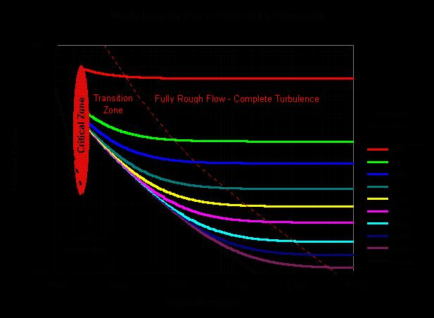
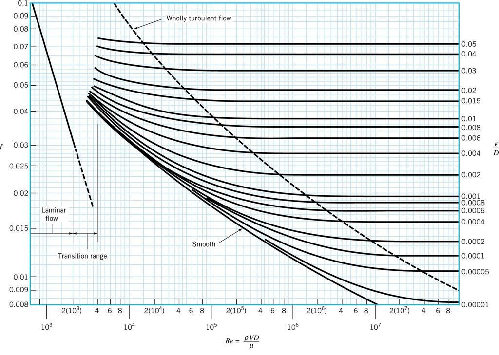
42 Moody diagram A convenient chart was prepared by Lewis F. Moody and commonly called the Moody diagram o riction actors or pipe low, There are 4 zones o pipe low in the chart: A laminar low zone where is simple linear unction o N R A critical zone (shaded) where values are uncertain because the low might be neither laminar nor truly turbulent A transition zone where is a unction o both N R and relative roughness A zone o ully developed turbulence where the value o depends solely on the relative roughness and independent o the Reynolds Number

43 43

44 Laminar

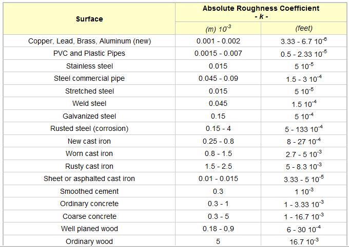
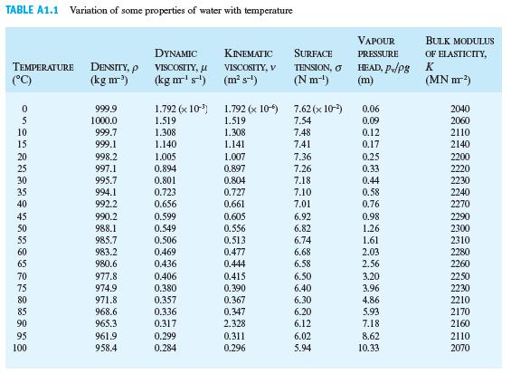
45 Typical values o the absolute roughness (e) are given in table 3. 45

46 46

47 Notes: Colebrook ormula is valid or the entire nonlaminar range (4000 < Re < 0 8 ) o the Moody chart log e / D Re In act, the Moody chart is a graphical representation o this equation 47

48 48

49 Problems (head loss) Three types o problems or uniorm low in a single pipe: Type : Given the kind and size o pipe and the low rate head loss? Type : Given the kind and size o pipe and the head loss low rate? Type 3: Given the kind o pipe, the head loss and low rate size o pipe?

50 Example The water low in Asphalted cast Iron pipe (e = 0.mm) has a diameter 0cm at 0 o C. Flow rate is 0.05 m 3 /s. determine the losses due to riction per km Type : Given the kind and size o pipe and the low rate head loss? 0.05m /s 3 π/4 0. m.59m/s T 0 o C υ.00 6 m /s e 0.mm e D N R 0.mm mm D Moody = 0.08 h L D g.55 m 000, m m m/s 50

51 The water low in commercial steel pipe (e = 0.045mm) has a diameter 0.5m at 0 o C. Q=0.4 m3/s. determine the losses due to riction per km T N R e D 0.50 Moody 0.03 Example Type : Given the kind and size o pipe and the low rate head loss? h m / km Q m / s A

52 Use other methods to solve - Cole brook k s ln 3.7D Re 0.86 e ln 3.7D N.5 R o k 0.5log s D e 5.74 R log ln R e h m / km

53 Cast iron pipe (e = 0.6), length = km, diameter = 0.3m. Determine the max. low rate Q, I the allowable maximum head loss = 4.6m. T=0 o C h F L D g Example 3 Type : Given the kind and size o pipe and the head loss low rate? N e D R T

54 Trial eq 0.0 eq e D N Moody R m/s N R Trial eq 0.0 eq e D N Moody R m/s 5 = 0.8 m/s, Q = *A = m 3 /s

55 Example 3.5 Compute the discharge capacity o a 3-m diameter, wood stave pipe in its best condition carrying water at 0oC. It is allowed to have a head loss o m/km o pipe length. Type : Given the kind and size o pipe and the head loss low rate? Solution : h L D g gh L / D / (9.8) 0. Table 3. : wood stave pipe: e = mm, take e = 0.3 mm e D At T= 0 o C, =.3x0-6 m /sec D N R

56 Solve by trial and error: Iteration : 0. Assume = m/ sec 0.0 N R From moody Diagram: 0. 0 Iteration : update = 0.0 N R m/ sec From moody Diagram: Iteration N R Convergence Solution: Q 3.5 m/s 3 A m /s

57 Alternative Method or solution o Type problems N R D 3/ Type. Given the kind and size o pipe and the head loss gh L / low rate? Determines relative roughness e/d Given N R and e/d we can determine (Moody diagram) Use Darcy-Weisbach to determine velocity and low rate Because is unknown we cannot calculate the Reynolds number However, i we know the riction loss h, we can use the Darcy-Weisbach equation to write: h L gh / / D D g L We also know that: N R 3/ / D gh L Re D / Can be calculated based on available data Re unknowns / D 3 / gh L Quantity plotted along the top o the Moody diagram /

58 Relative roughness e/d Moody Diagram N R 3/ / D gh L / Resistance Coeicient Fully rough pipes Smooth pipes Reynolds number

59 Example 3.5 Compute the discharge capacity o a 3-m diameter, wood stave pipe in its best condition carrying water at 0oC. It is allowed to have a head loss o 3m/km o pipe length. Type : Given the kind and size o pipe and the head loss low rate? Solution : At T= 0 o C, =.3x0-6 m /sec N R D 3/ gh L / 3 (3).30 6 (9.8)(3) Table 3. : wood pipe: e = mm, take e = 0.3 mm From moody Diagram: 0. 0 h L D g gh L / D / 3.5m /sec, 5 e D Q A m /s

60 = 0.0

61 Example (type ) H L H = 4 m, L = 00 m, and D = 0.05 m What is the discharge through the galvanized iron pipe? Table : Galvanized iron pipe: e = 0.5 mm e/d = /0.05 = = 0-6 m /s We can write the energy equation between the water surace in the reservoir and the ree jet at the end o the pipe: h L g h p g h p g D L g D L g

62 Example (continued) Assume Initial value or : o = 0.06 Initial estimate or : Calculate the Reynolds number m/sec N R D Updated the value o rom the Moody diagram = m/sec N R D Iteration N R Solution: Convergence 0.84 m/s Q A m 3 /s

63 Initial estimate or A good initial estimate is to pick the value that is valid or a ully rough pipe with the speciied relative roughness o = 0.06 e/d = 0.003

64 Solution o Type 3 problems-uniorm low in a single pipe Given the kind o pipe, the head loss and low rate size o pipe? Determines equivalent roughness e Problem? Without D we cannot calculate the relative roughness e/d, N R, or N R Solution procedure: Iterate on and D. Use the Darcy Weisbach equation and guess an initial value or. Solve or D 3. Calculate e/d 4. Calculate N R 5. Update 6. Solve or D 7. I new D dierent rom old D go to step 3, otherwise done

65 Example (Type 3) A pipeline is designed to carry crude oil (S = 0.93, = 0-5 m /s) with a discharge o 0.0 m 3 /s and a head loss per kilometer o 50 m. What diameter o steel pipe is needed? Available pipe diameters are 0,, and 4 cm. From Table 3. : Steel pipe: e = mm Darcy-Weisbach: L h D g D 6 LQ g h /5 h D L D Q A L D Q 4 5 g g D D g Make an initial guess or : o = 0.05 /5 4 / LQ /5 D / m Now we can calculate the relative roughness and the Reynolds number: e D N R D D Q A 3 D 4Q D D 4Q D D update = 0.0

66 Updated estimate or = 0.0 e/d =

67 Example Cont d D /5 N R D From moody diagram, updated estimated or : = 0.0 D = 0.03 m N R e D update Solution: D = 0.03m Use next larger commercial size: D = cm Iteration D NR e/d Convergence

68 Example 3.6 Estimate the size o a uniorm, horizontal welded-steel pipe installed to carry 4 t 3 /sec o water o 70 o F (0 o C). The allowable pressure loss is 7 t/mi o pipe length. Solution : From Table : Steel pipe: e = mm Darcy-Weisbach: h L L D Q A D Let D =.5 t, then g /5 /5 h L L D 4.33 /5 = Q/A =.85 t/sec Q A g L D Q 4 g D 6LQ 4 D 5 g 8 LQ D g a h L Now by knowing the relative roughness and the Reynolds number: e D N R D *.5 6.6* *0 5 We get =0.0 /5

69 A better estimate o D can be obtained by substituting the latter values into equation (a), which gives /5 /5 D * t A new iteration provide = 4.46 t/sec N R = 8.3 x 0 5 e/d = = 0.0, and D =.0 t. More iterations will produce the same results.

70 Simpliied Hazen-Williams D 5cm.38C Empirical Formulas HW R 0.63 h 3.0m / sec 0.54 S British Units 0.85C HW R 0.63 h S 0.54 SI Units R S C h HW hydraulic Radius h L Hazen Williams wetted A wetted P Coeicien t D 4 D D 4 h C HW 0.7 L. 85 Q D SI Units

71

72 Empirical Formulas Manning Formula This ormula has extensively been used or open channel designs It is also quite commonly used or pipe lows 7

73 Simpliied Manning n R /3 h S / R h hydraulic Radius h S L n Manning Coeicien t wetted A wetted P D 4 h 0.3 L D 5.33 nq SI Units 73

74 n R / 3 h S / h h 0.3n L D Q 6/ n.33 D L n = Manning coeicient o roughness (See Table) R h and S are as deined or Hazen-William ormula. 74

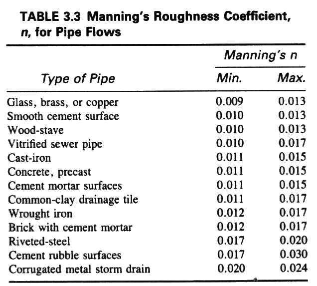
75 75

76 The Chezy Formula / / h C R S h L 4 D C where C = Chezy coeicient 76

77 It can be shown that this ormula, or circular pipes, is equivalent to Darcy s ormula with the value or 8g C [ is Darcy Weisbeich coeicient] The ollowing ormula has been proposed or the value o C: C [n is the Manning coeicient] S n n ( 3 ) S R h 77

78 The Strickler Formula: k R S str / 3 / h h 6.35 D L.33 k str where k str is known as the Strickler coeicient. Comparing Manning ormula and Strickler ormula, we can see that n k str 78

79 Relations between the coeicients in Chezy, Manning, Darcy, and Strickler ormulas. k str n /6 C k str R h n Rh 8g /3 79

80 Example New Cast Iron (C HW = 30, n = 0.0) has length = 6 km and diameter = 30cm. Q= 0.3 m3/s, T=30 o. Calculate the head loss due to riction using: a) Hazen-William Method h h C 0. 7 L. 85 HW D Q m b) Manning Method h h 0.3 L D nq m

81 8

82 Minor losses It is due to the change o the velocity o the lowing luid in the magnitude or in direction [turbulence within bulk low as it moves through and itting] Flow pattern through a valve 8

83 The minor losses occurs due to: alves Tees Bends Reducers And other appurtenances It has the common orm h m k L Q kl g ga minor compared to riction losses in long pipelines but, can be the dominant cause o head loss in shorter pipelines 83

84 Losses due to Contraction A sudden contraction in a pipe usually causes a marked drop in pressure in the pipe due to both the increase in velocity and the loss o energy to turbulence. Along wall Along centerline h c k c g

85 alue o the coeicient K c or sudden contraction

86 Max Head Loss Due to a Sudden Contraction h K L L g h c 0.5 g 86

87 Head losses due to pipe contraction may be greatly reduced by introducing a gradual pipe transition known as a conusor Figure 3. k c ' h c ' k c ' g

88 Losses due to Enlargement A sudden Enlargement in a pipe ( h E g )

89 Note that the drop in the energy line is much larger than in the case o a contraction abrupt expansion gradual expansion smaller head loss than in the case o an abrupt expansion

90 Head losses due to pipe enlargement may be greatly reduced by introducing a gradual pipe transition known as a diusor h E ' k E ' g

91 Loss due to pipe entrance General ormula or head loss at the entrance o a pipe is also expressed in term o velocity head o the pipe h ent K ent g 9

92 Head Loss at the Entrance o a Pipe (low leaving a tank) Reentrant (embeded) K L = 0.8 Sharp edge K L = 0.5 Slightly rounded K L = 0. Well rounded K L = 0.04 h K L L g 9

93 Dierent pipe inlets increasing loss coeicient

94 Another Typical values or various amount o rounding o the lip 94

95 Head Loss at the Exit o a Pipe (low entering a tank) K L =.0 K L =.0 h L g K L =.0 K L =.0 the entire kinetic energy o the exiting luid (velocity ) is dissipated through viscous eects as the stream o luid mixes with the luid in the tank and eventually comes to rest ( = 0). 95

96 Head Loss Due to Bends in Pipes h b k b g R/D K b

97 Miter bends For situations in which space is limited, 97

98 Head Loss Due to Pipe Fittings (valves, elbows, bends, and tees) h K v v g 98

99 99

100 The loss coeicient or elbows, bends, and tees 00

101 Loss coeicients or pipe components (Table)

102 Minor loss coeicients (Table)

103 Minor loss calculation using equivalent pipe length L e k l D

104 Energy and hydraulic grade lines Unless local eects are o particular interests, the changes in the EGL and HGL are oten shown as abrupt changes (even though the loss occurs over some distance)

105 Example In the igure shown below, two new cast iron pipes are in series, D =0.6m, D =0.4m, length o each pipe is 300m, level at A =80m, Q = 0.5m3/s (T=0 o C). There is a sudden contraction between Pipe and, and Sharp entrance at pipe. Find the water level at B? e = 0.6mm v = Q = 0.5 m3/s

106 exit c ent L B A h h h h h h h Z Z g k g k g k g D L g D L h exit c ent L sec sec ,. D,. D,. υ D R,. υ D R, m/.. π. A Q, m/.. π. A Q moody moody e e 0.7,.5, 0 exit c ent h h h Solution

107 m. g. g.. g.. g.... g.... h Z B = = m g k g k g k g D L g D L h exit c ent L

108 Example A pipe enlarge suddenly rom D=40mm to D=480mm. the H.G.L rises by 0 cm calculate the low in the pipe

109 s m A Q s m g g g g A A g g g z g p z g p h g g h z g g p z g g p L L / / Solution

110 Note that the above values are average typical values, actual values will depend on the manuacturer o the components. See: Catalogs Hydraulic handbooks!! 0