Incorporating Temporal and Country Heterogeneity in. Growth Accounting - An Application to EU-KLEMS

Transcription

1 Incorporating Temporal and Country Heterogeneity in Growth Accounting - An Application to EU-KLEMS A. Peyrache (a.peyrache@uq.edu.au), A. N. Rambaldi (a.rambaldi@uq.edu.au) CEPA, School of Economics, The University of Queensland, St Lucia, Brisbane, QLD, 40, Australia. Abstract We introduce a general model for the specification and estimation of group specific trends and time varying slopes in pooled time series regressions (fixed N, large T). The model nests a number of commonly used panel data models introduced in the literature which deal with group specific trends. The econometric model is represented in state-space form. We provide a production frontier interpretation of this group specific temporal variation and derive a postestimation growth accounting to provide a quantitative assessment of the main factors behind sectoral labour productivity growth. We make use of the EU-KLEMS dataset, covering the period for 13 countries and 0 sectors of each economy. Keywords: time trends, panel data, state-space, sectoral productivity, Malmquist JEL Classification: C13, C, C3, O4. 1 Introduction In this paper we write the production model as a general framework that provides a venue to deal with group specific trends (temporal variation in individual heterogeneity) and time variation (trends) in the vector of slope coefficients in parametric pooled time series production models. By 1

2 pooled time series models we mean that the size of the cross section N is fixed (one may think of this as a panel data with fixed N and long T ). The simpler example of a pooled time series is when dealing with country level analysis where the number of countries in the world is fixed (fixed N )andthesamplehasthenatureofatimeseriesforeachcountry. Inotherwords,ateachtime period one observes the population in the cross sectional dimension. This simple fact poses some challenges because the estimator used must possess asymptotics for large T, ratherthanlargen (as it is usually the case with many panel data estimators). In fact, large N asymptotics will not work in this case because of the very nature of the data (i.e. N is fixed). We make two main contributions. First, we develop a general econometric representation of the production model and then show that it is able to nest a number of commonly used panel data models introduced in the literature which deal with group specific trends. We present the model in a primal setting (i.e. a production function instead of a cost function), where the production function is assumed to have time-varying parameters and time-varying technical inefficiency. We write this general model in its state-space representation which provides the venue to write the likelihood function for the unknown parameters as well as an estimation framework with established properties via the Kalman filtering algorithms. Second, we develop a growth accounting decomposition based on the estimated production function in order to separate productivity change from inputs growth effects. This allows us to identify the main drivers behind observed labour productivity growth. The framework is illustrated using the EU-KLEMS dataset to identify the main trends (and biases) in productivity growth in the period for 13 OECD countries and 0 industrial sectors of each economy. The approach we propose has the advantage of allowing individual country heterogeneity to be correlated with the regressors. For example, in a production frontier framework, when the level of total factor productivity (TFP) is correlated with the inputs, the standard OLS estimator of the parameters of the production function will return biased estimates. Due to the obvious link between the framework proposed here and the stochastic frontier literature, we start by framing our work in this specific setting. The classical stochastic frontier model (SFM) introduced by Aigner et al (199) and Meeusen and van den Broeck (19) is well

3 established in cross-sectional settings with the main purpose of allowing one-sided deviations from the production frontier (regression line). From a historical perspective, this attempt should be contrasted with classical regression analysis where firms or countries were assumed to be perfectly efficient and any deviation from the regression line was attributed to noise. The interest in SFM as a tool for efficiency analysis came later thanks to the contributions of Jondrow et al (198) and Battese and Coelli (1988). A first discussion of panel data settings for SFM was provided by the seminal paper of Schmidt and Sickles (1984), although under the restrictive assumption of time invariant technical efficiency. In such a context technical efficiency can be interpreted as unobserved heterogeneity and panel data estimators are available to deal with it. Once the literature started to think in a panel data setting, the path was open to productivity measurement. As emphasized by Lovell (199) in a review of the issue, nonparametric methods (such as DEA) accommodated productivity measurement in a more satisfactory way than SFM. In fact, in a dynamic context of productivity measurement, one has to model at least two different contributors to productivity change: technical change and technical efficiency change. While the latter has been addressed widely, the former has been basically left to ad hoc solutions and, in a sense, SFM analysis has been biased towards the static (efficiency measurement) and not the dynamics (productivity measurement). Kumbhakar (1990, 004) proposed a model with deterministic time varying technical inefficiency and Battese and Coelli (199) parameterized the deterministic function of time in a different fashion. At the same time Cornwell et al (1990) proposed to accommodate for time varying technical inefficiency using quadratic time varying firm specific intercepts. Ahn et al. (000) proposed to model technical inefficiency as an AR(1) process (stationary) and the same route was followed, with some interesting novelties, by Desli et al. (003) and Tsionas (00). All these specifications place their emphasis on technical efficiency change, with less attention to technical change. Particularly, stationary specifications (like the AR(1)) are unlikely to perform well when modeling a structurally non-stationary phenomena like technical change. Thus, it is not surprising that technical change has been accommodated by the applied researcher using ad hoc methods. Acommonwayofaddressingsuchaneventisintroducingtimeasanexplanatoryvariableinthe regressor vector of inputs, possibly having it interacting with the inputs to provide the second order 3

4 approximation typical of translog functional specifications. This is indeed the way explicitly put forward by Orea (00) to build up the generalized Malmquist productivity index. This strategy has been also proposed by Coelli et al (003) and Ahn et al (000). Closer to our approach are a number of recent works. Jin and Jorgenson (009) recently introduced a state-space representation of a cost function where constant time trends (usually used to describe the rate and biases in technical change) are replaced by latent variables. Their work is mainly concerned with single time series. Emvalomatis et al (011) propose a modelling framework to estimate dynamic efficiency in a panel. Their econometric formulation models time varying inefficiency in a non-linear fashion and provides a Kalman filtering procedure to estimate the model. Our framework is closer in spirit to the recent work of Kneip et al (01) who present a strategy based on a semi-parametric specification which uses common factors to accommodate cross-sectional time varying heterogeneity. The production model The production technology is represented via a production function where a single output y it (log of output) is produced by means of multiple inputs X it where i =1,...,N indexes the number of countries, t =1,...,T indexes the number of time periods. A translog specification is assumed and thus X it is a 1 k vector containing the log of inputs, the squared log of inputs and interaction terms: y it = µ t + it + X it t + it (1) In this specification µ t, t are time varying parameters common to all the countries, it is a country specific time varying intercept (group specific time trend) and it is a normally distributed error term. The country specific intercepts are given by µ t + it = a it. In order to identify all P the parameters we need to assume 1 N i a it = µ t,sothatµ t represents the time variation in the average intercept (it is an average function or common shock). This leads to the following possible reparameterization of the model: 4

5 y it = a it + X it t + it () Since technical efficiency can be interpreted as a shift in the intercept, Schmidt and Sickles (1984) proposed also to reparameterize equation () using the following transformation: max {a it} = i=1,...,i a t, u it = a it a t (this is a measure of technical inefficiency) which returns the following stochastic production frontier: y it = a t + X it t u it + it (3) The production frontier embedded in (3) is time varying (due to the time varying coefficients (a t, t)) andtechnicalinefficiencyistimevarying(asanotationalconvenienceweusea t for the maximum intercept and a it = a t u it for the country specific intercept). If one is willing to assume no technical change then the production frontier becomes time invariant y it = a + X it u it + it ; going a step further and assuming also time invariant technical inefficiency one obtains the model discussed by Schmidt and Sickles (1984) in their seminal paper as a special case of specification (1): y it = a + X it u i + it (4) In equation (4) the technology is fixed (no technical change as the parameters are fixed) and the technical efficiency term is a fixed effect unobserved heterogeneity component. It is possible to estimate such a model using standard panel data estimators (for a detailed discussion of this point see Schmidt and Sickles, 1984). Of course, the validity of such a procedure is predicated on the assumption that technical efficiency is time invariant and this is a tolerable assumption for short panels. On the other hand, when T becomes larger the time invariant technical efficiency and no technical change model becomes less appealing. In this paper we propose a time-varying parameters specification which provides a general formulation of technical change nesting the standard practice of including deterministic time trends as a special case. Specification (3) emphasizes that there is always at least one country that lies onto the international production frontier and this country is the one with the maximum value of the intercept. This assumption leads to two fundamental 5

6 advantages: first, technical change can be easily and elegantly modeled as a stochastic trend instead of being forced to be deterministic as in the standard practice; second, theonesided technical inefficiency variable is free from any assumption about its statistical distribution and free to move according to the stochastic trend specification. Although reparameterizations () and (3) are useful in terms of interpretation, we will use model specification (1) for estimation purposes. Parameterization (3) provides the post-estimation interpretation of the coefficients of our proposed econometric model from which the main components of productivity change can be recovered (this is discussed in detail in Section 5) 3 A General Representation of the Production Model 3.1 The General Econometric Model In this section we develop a general econometric model and return to its stochastic frontier representation in Section 5. The purpose of this general model is to show that a number of the panel production models commonly estimated in the literature are nested in this representation. While in practice one of the nested members is likely to be a best fit for a given emprical application, one advantage of the representation is to provide a framework for model specification, as members of the family can be compared through the use of criteria such as the AIC or SBC. In this general representation noise is accommodated with the standard normally distributed two-sided disturbance ( it N (0, )). The country specific intercept moves in time due to the time varying common average µ t and the country specific trend it. The common shock µ t is represented by a stochastic double trend specification (random walk with time varying drift): µ t = c µ + t 1 + µ t 1 + µt (5) t = c + t 1 + t where µt and t are independent innovations assumed to be normally distributed µt N 0, µ and t N (0, ). This stochastic double trend specification (with drifts c µ and c )isabletonestthecommonpracticeofusingdeterministicquadratictrends.ifbothvariances,

7 µ and, are zero the trends are deterministic (see Harvey (00) Section.3). The time varying country specific shock it is assumed to follow a country specific stochastic double trend with drifts: t = c + t 1 + t 1 + t t = c + t 1 + t () where t is a N 1 vector, t is a N 1 vector and the other vectors dimensionality are defined by conformability. The innovation vectors are normally distributed: t N 0, I N 1 and t N 0, I N 1. The last piece of our model is the vector of slope coefficients which models the bias in technical change. They are assumed to move according to a double stochastic trend with drifts: apple where, by conformability, = 1... K t = c + t 1 + t 1 + t () t = c + t 1 + t 0 is a K 1 vector of drifts, t N 0, I K 1 the vector of innovations and t N (0, I K 1 ). Putting equations (5), () and () together, the full model representation will be: y t = t +1 N µ t + X t t + t t = c + t 1 + t 1 + t t = c + t 1 + t µ t = c µ + t 1 + µ t 1 + µt (8) t = c + t 1 + t t = c + t 1 + t 1 + t t = c + t 1 + t In this model the variance of the country specific intercept comes from two different sources: first, a common shock to all the countries and, second, from a country specific shock. This is a general model able to nest some of the commonly used models in the literature. To show this it

8 will be convenient to write (8) in what is known as its state-space representation, y t = Z t t + t t = D t 1 + c t + t (9) apple 0 apple where t = t t µ t t t t, Z t = I N 0 N N 1 N 0 N X 0 N K, apple 0 c t = c c c µ c c c and D is a comformable matrix of zeros and ones (see Appendix A.1). The vector t has size ( t )=(N + K +1) = B and it is known as the state-vector in the state-space literature (the reader is referred to Harvey (1989, 00), Durbin and Koopman (01) for detailed discussion of how econometric models can be represented in state-space form). As the vector c is also size B, thereareatotalof4(n + K +1) = B parameters (plus covariance parameters) to be estimated (Section 4). For the purpose of estimation a more convenient reparameterisation of the state-space is given by the following transformation to the state vector t : t = 4 t tc c 3 5 (10) where the matrix t is defined as (see Appendix A.1 for the derivation and the final form of t): t = P t 1 j=0 Dj = I + D + D D t 1 (11) After the transformation the state space becomes: y t = Z t t + t (1) where Z t = apple Z t (Z t t ), D = t = D t 1 + t (13) 4 D 0 0 I 3 5, t = 4 t 0 3 5, E( t 0 t )=Q and E( t 0 t)= H. There are two advantages of this representation, the first is that we can now show that it 8

9 nests a number of other models and second that we can now use standard state-space estimation algorithms. That is, we can write the likelihood function to estimate all covariance parameters (i.e. those parameters in Q and H) aswellasthestatevector, t,anditscovariancematrix,p t, through the use of the Kalman filter and Kalman smoothing algorithms. 3. Nested models Our model specification (8), although very general, is not very parsimonious since requires estimation of 4(N + K +1) parameters plus all parameters in Q and H using N T observations. Thus, unless T is very long, some restrictions on the model are needed in order to improve its finite sample estimation performance. This is also a useful exercise, since it gives us the possibility of discussing some commonly used models as special cases of specification (8). We introduce a generic set of J linear restrictions on the parameters of the model: R t t = r t (14) and focus our attention on the set of restrictions which fix r t =0. The following four restricted models will be discussed in detail in this section: 1) the fixed effects time invariant model; ) fixed effects with common deterministic time trend model; 3) the Cornwell et al (1990) model (which includes the quadratic specification of Battese and Coelli, 199); 4) a simple stochastic time-varying model Fixed effects (FE) and fixed effects deterministic time trend model (FEDT) One way of dealing with technical inefficiency in panel data frameworks is to treat it as unobserved heterogeneity (time invariant) as in specification (4). This approach has been discussed, for example, by Schmidt and Sickles (1984) and by Sickles (005) in his review. By setting Q =0(see (13)), and defining R t as follows: R t = 4 0 (N+) N I N+ 0 (N+) (K+B) 0 (K+B) (+N+K) I K+B 3 5 9

10 one obtains the following restrictions: 4 t t tc tc µ t tc µ t(t 1) c t c tc 3 =0 5 The last B restrictions impose all elements of c to be zero. The other restrictions impose t =0, µ = =0, =0. Then the general model is restricted to a standard time invariant fixed effects model: y t = t + X t t + t t = t 1 = t = t 1 = It is then easy to see that the general specification (8) collapses to (4), where technical inefficiency is unobserved heterogeneity and the parameters of the production function are time invariant. In such a framework, one can attempt to accommodate technical change by introducing deterministic time varying parameters. A common (and simple) procedure is to treat time as a standard variable in the translog specification (i.e., adding time and its interaction with inputs as additional regressors). This model implicitly assume the following deterministic time varying coefficients: it = t + t u i nt = n0 + n t, n =1,...,N and can be obtained by setting Q =0(see (13)) and defining R t as follows, R t = 4 0 N N I N 0 N (+K+B) 0 (N+K) (+N+K) I N+K 0 (N+K) (+K) 0 K (B++N+K) I K

11 obtaining the following model: y t = t +1 N µ t + X t t + t t = t 1 µ t = c µ + t 1 + µ t 1 t = c + t 1 t = c + t 1 Under these weaker restrictions the equation for the country specific intercept in (8) collapses to µ t + i,i=1,...,n and the common time trend follows a deterministic quadratic trend specification. If, additionally, =0the intercept deterministic time trend becomes linear (which is a quite common way of dealing with trends, i.e. Hicks neutral linear deterministic time trend). 3.. The Cornwell Schmidt and Sickles (1990) model (CSS) Cornwell et al. (1990) proposed to model the country specific time-varying intercepts as country specific deterministic quadratic time trends. Their model is: y it = it + X it + it with it = 0i + 1i t + i t. This can be easily accommodated by our formulation (8) imposing the restrictions Q =0(see (13)) and defining R t as, R t = 4 0 N I 0 (K+B) 0 K (+N+K) I K 0 K B 0 (+K) (B+N) I +K

12 These restrictions imply the following model: y t = t + X t t + t t = c + t 1 + t 1 t = c + t 1 t = t 1 and impose a country specific deterministic quadratic time trend on the time varying intercepts (this is easy to show 1 and it is a well known result, Harvey (00)). The Battese and Coelli (199) model Battese and Coelli (199) presented a very popular way of introducing time varying inefficiency. The technology is fixed (i.e., no technical change) and changes in the country specific intercepts will come from the time varying technical inefficiency. Technical inefficiency will vary as a deterministic function of time: u it = (t)u i. They first propose an exponential function for (t) which, as the authors note, is very rigid. To remedy this problem, they propose a quadratic specification: (t) = (t T )+ (t T ). This function can be expressed as (t) =( 0 1 T + T )+( 1 T ) t + t, which is a quadratic deterministic time trend specification for the time varying intercepts. It is easy to see that this specification is a special case of the Cornwell et al (1990) model where the firm specific time varying parameters are different but proportional to each other, i.e.: i / j We note that the Battese and Coelli (1990) specification is restrictive in the sense that inefficiency follows the same trend for all the firms, while the Cornwell et al (1990) specification is able to accommodate different patterns (at the cost of increasing enormously the number of parameters to be estimated). Since Battese and Coelli (1990) is nested in Cornwell et al (1990), it follows that it is also nested in our general model specification. 1 See Appendix of the Working Paper version - *** (deleted for referring process) 1

13 3..3 A simple stochastic trend model (TV) In order to reach a good balance between flexibility (statistical fitting) and parsimony (low number of parameters), we present another nested model. As a starting point it should be noted that the general formulation (8) requires the estimation of 4(N + K +1) parameters using N T observations, therefore, unless T is very large, the estimation will be very imprecise as the model is flexible but not parsimonious. A similar problem arises with the Cornwell et al (1990) model, where the number of parameters is equal to 3N + K (with the time invariant slope parameter formulation). On the contrary the Battese and Coelli (199) and Fixed effects models are very parsimonious but quite inflexible. The specification is given in (15) and it is obtained under the following restrictions to (8): 3 Q = 4 I N 0 (N+) (N+) I K 5 0 K K R t = 4 0 (N+) N I N+ 0 (N+) (K+B) 0 (K+B) (N++K) I K+B 3 5 y it = it + X it t + t it = it 1 + it (15) t = t 1 + t Here the common shock is suppressed (although this saves only 4 parameters) and all the drifts are suppressed (there is no deterministic trend in this model). This basically means estimating N + K parameters with N + T observations, which is quite reasonable. Moreover the stochastic time trend formulation is flexible enough to accommodate many different types of trends in the data. 13

14 4 Estimation In our model (1) the local level, slope, t, (which captures individual country specific trends) and the t can be correlated with X t and thus our modelling framework is an extension of the fixed effects model to the case of time-varying parameters (This is further discuss in Appendix A.). The parameters of the general production model are those in the state-space representation (1) and (13). To estimate any of the nested members of the family (as shown in the previous section) one can incorporate the corresponding set of restrictions and estimate the corresponding statespace form. However, computation can be approached also by estimating each nested model (ie FE, FEDT, CSS, Battese and Coelli (199), TV, etc.) using other estimation approaches that are consistent for that model. The importance of the results presented in Section 3 is that we show is possible to make a systematic statistical comparison among them using the AIC and BIC measures of fit. The two measures are: AIC = log e0 e NT + K, BIC = log e0 NT e NT + K log NT. We use these NT measures of statistical fit in order to penalize for the loss in degrees of freedom of models with a high number of parameters, and in Section..1 we provide the results of the estimation of the production model using these as alternative model specifications and can compare them via the computed values of the criteria. For the estimation of the parameters in specifications FE, FEDT, CSS and Battese and Coelli (199) the reader is referred to the original papers. Estimation of the general model as well as any of the nested members of the family in their state-space form is standard, and descriptions of the classical as well as Bayesian approach can be found in Harvey (1989) and Durbin and Koopman (01). The properties of the Kalman filter/smoother as an estimator are also presented in these sources. In the interest of completeness we describe the estimation of the one of the members of the nested family, the simple TV model presented in Section 3..3, in Appendix A.3. 5 Growth accounting The general production model proposed here, (1), is a time-varying parameter model, and this has some consequences for the measure of productivity which have to be considered. The first obvious 14

15 difference is that time enters the production function via the time-varying parameters and not as a standard explanatory variable in the translog specification. This means that the functional specification we are dealing with is more general than the standard translog specification. In fact, it is a translog production function at any point in time, but it allows the parameters to move in time in a non-translog way. One of the consequences of this modelling strategy is that the quadratic identity lemma (Diewert, 19) can be applied only at a given point in time, i.e. only to the input variables and not to the time variable. Since productivity is something that happens in time, the lemma cannot be used to build the translog productivity index in the spirit of Orea (00). Therefore we have to re-build a measure of productivity growth. We assume that standard symmetry conditions of the translog specification holds at any point in time. In order to build a measure of productivity, let us consider the difference in output between two time periods using the reparameterization of the production model in (): y it+1 y it = a it+1 + X it+1 t+1 a it X it t (1) This observed change can be imputed to three different effects: i) the shift in the country specific intercept, ii) the shift in the slope parameters and iii) the growth in the inputs. The first two effects are what one usually refers to as productivity change, while the last effect is an input growth effect. To isolate the productivity effect from the input growth effect we use a Malmquist logic, keeping some of the variables fixed while moving the others in order to separate the relative contribution of the different effects. Productivity growth can be measured keeping the level of inputs at the base period level, obtaining the equivalent of the base period Malmquist productivity index: TFP t = a it+1 a it + X it ( t+1 t ) (1) Keeping the level of inputs at the comparison period value, we obtain the equivalent of the comparison period Malmquist productivity index: TFP t+1 = a it+1 a it + X it+1 ( t+1 t ) (18) 15

16 and to avoid the arbitrariness of choosing the base, we use the geometric mean of these two indexes in order to get an index of productivity growth: TFP = 1 (TFPt + TFP t+1 )= = a it+1 a it + 1 (X it + X it+1 )( t+1 t ) (19) The input growth effect or factor accumulation effect (FA) can be computed using the same logic. The base period index is: FA t =(X it+1 X it ) t (0) The comparison period index is: FA t+1 =(X it+1 X it ) t+1 (1) Finally, we use the geometric mean as a measure of the input growth effect: FA = 1 (FAt + FA t+1 )= 1 ( t + t+1 )(X it+1 X it ) () It is easy to verify that the two effects are an exhaustive and mutually exclusive decomposition of the log change in output: y it+1 y it = TFP + FA (3) Therefore TFP has the standard interpretation of being the difference between output growth and input growth between two time periods. TFP growth can be further attributed to two very different components: first the change in the country intercept UTC = a it+1 a it and second the bias in technical change deriving form the time variation of the slope coefficients: BTC = 1 (X it+1 + X it )[ t+1 t] (4) Thus the overall growth accounting decomposition is given by: y it+1 y it = TFP + FA = UTC + BTC + FA (5) 1

17 where UTC + BTC = TFP.Allthesecomponentsarecountryandtimespecific.Apositive (negative) BTC measures the extent to which technical change has been biased (for example, capital-using or capital saving). UTC incorporates the effect of the change in the country specific intercept (which is a measure of the productivity level). FA is the contribution of the increase (decrease) in the inputs endowment. We note that this decomposition is exhaustive (does not leave any residual) and the different components are independent from each other. In fact, UTC and BTC depends on different coefficients of the model and FA depends on how much a country is investing and accumulating factors of production. We compute the elements of (5) in the empirical section. Empirical Application.1 Data The EU-KLEMS dataset is an official project that collects input and output data on prices and quantities for industrialized countries in the time span (see O Mahony and Timmer (009)). For each industry the database provides value data on gross output, capital compensation, intermediate inputs (materials and energy) along with fixed base price and quantity index numbers (1995=100). We used the amount of total hours worked by persons engaged as a proxy for the quantity of labour (the alternative of using the number of persons engaged is less satisfactory). Since gross output, intermediate inputs and capital services are measured in local currencies we used PPPs to adjust for cross-sectional differential in the general level of prices. PPPs indexes use US as benchmark (US=100, 1995=100), are sector specific (i.e., each sector has different PPPs) and different for sectoral output, intermediate inputs and capital services (i.e., there are three sets of PPPs). Due to lack of data (missing values) we limit our attention to a subset of data, specifically 13 countries and 0 industrial sectors in the time span The list of countries and sectors is reported in Table 1. [Table 1 here] 1

18 We build a balanced panel dataset in the following way. Be j =1,...0 the sector and i =1,...13 the country, then the index of sectoral output for country i at time t Y j it is: Y j it = GOj i1995 PPP j I j it () i where GO j i1995 is the value of gross output in 1995 for sector j in country i; Ij it is the fixed base index of sectoral output quantity change between time t and the base period 1995; PPP j i is the purchasing power parity of country i in sector j. Withasimilarprocedurequantityindexnumbers are built for intermediate output (materials) and capital services. With this procedure we obtain a true balanced panel data set where cross-sectional (cross-country) comparability is built using PPPs and time comparability is built using fixed base quantity index numbers. This procedure guarantees that in each time period countries can be compared. The result is a quantity index number that proxies sectoral output production, a quantity index number proxying capital services, aquantityindexnumberthatproxiesthelevelofmaterialsusedandthenumberofhoursworked for the labour input. All the variables obtained with this procedure have been normalized by the sample minimum. The usual procedure of normalizing variables by sample mean is very unfruitful in our modelling setting. In fact, consider that the sign of the capital bias component depends on: the sign of [ kt+1 kt] that is common to all countries and the sign of (log k it+1 +logk it ) that is country specific. Now, if we normalize by the sample mean for a positive (negative) sign of [ kt+1 kt] the countries below the sample mean will have a negative (positive) capital bias, while the countries above the mean will have a positive (negative) capital bias. This is unreasonable, since although the magnitude of the capital bias should be proportional to the quantity of capital used, it should be monotonic for all the countries, i.e. the same for all the countries. This is guaranteed by a transformation by the sample minimum.. Empirical Results To illustrate the flexibility and parsimony of our proposed framework we first present a comparison of the simple TV model to CSS, FE and FEDT models using statistical fitting criteria such as BIC, AIC and adjusted R. We then present a selection of point- and interval- estimates of the time- 18

19 varying parameters (local level intercept and slopes) as well as the computed growth accounting exercises. In our empirical model we assume constant returns to scale of the production function, expressing it in the intensive form: output per worker on the left hand side; capital per worker and materials per worker on the right hand side. We further assume for the TV model that second order parameters of the translog specification are time invariant. Consequently we have two time varying first order slope parameters and three time invariant second order slope parameters (in the TV specification): y it = a it + kt k it + mt m it + kk k it + mm m it + km m it k it + it where y is the log of output per worker, k is the log of capital per worker and m is the log of materials per worker. We estimate all the models separately for each of the 0 industrial sectors, thus applying them to each sectoral panel dataset individually...1 Comparison of the models In Table we provide AIC and BIC values (along with R-squared and AdjR-squared) for each model in each sector. The first thing to note is that the fixed effects model provides a very good fit of the data. In all sectors analyzed the R-square is above 90% and the corresponding AIC value below The fixed effects model is always the best performer in terms of both AIC and BIC criteria: the loss in statistical fitting (when compared to the other models) is always more than compensated by the lower number of parameters to be estimated. The second general pattern of these results is that our simple stochastic time trend model (TV) outperform the CSS model uniformly. The level of flexibility of the TV model is very close to the CSS model, but it is parsimonious to the extent that its performance is comparable to the fixed effects model. For example in sector Fuel (Coke, Refined Petroleum and Nuclear Fuel) the R-square of the TV model is equal to the R-square of the CSS model, although this fitting is reached with less parameters and this explains why the BIC and AIC statistics are so different. For this sector the AIC value of the CSS model is 0.8 against a of the TV model; interestingly enough the fixed effects, with a value of 0.101, has a performance very similar to the TV model. In terms of the BIC the 19

20 results are qualitatively the same, although (due to the stronger penalization for degree of freedom loss of the BIC) the differences are larger. The story in other sectors is very similar, leading us to conclude that the TV model represents a very good compromise between flexibility (statistical fitting) and parsimony (low number of parameters). In the following section we discuss the results on productivity change and growth accounting decomposition derived from the TV model. [Tablehere].. Patterns of growth Applying the TV econometric model to the 0 panel datasets (sectors) returns 0 time varying intercepts, 40 time varying slope coefficients and 540 growth accounting decompositions (one for each country, in each sector, in each time period). In order to make all this information manageable and interpretable, we decided to illustrate only the trends of 4 countries (US, Germany, Italy and Japan) and present the growth accounting exercise only for three sectors: Electrical and Optical Equipment, Post and Telecommunications, Chemicals. The first two sectors represent the most dynamic sectors in terms of productivity since they are the protagonists of the IT industrial revolution (basically computers and mobile phones). The last sector is interesting because it is a classical industrial sector and it illustrates well the notion of biased technical change. Results for all the other countries and all the other sectors are available on request. Figure 1 reports intercept trends for the selected countries in the Electrical and Optical Equipment sector. From this figure emerges clearly the US boom in the IT sector, with a consistently uptrending intercept. On the contrary the other selected countries do not show any clear trend and indeed present a quite stable pattern. For this sector we report in Figure the trends in the first order slope coefficients. Both the capital and materials coefficients are basically time invariant (the capital coefficient is not significantly different from zero, although the second order coefficients (not shown) are). This points out to a Hicks neutral productivity change in the Electrical and Optical Equipment sector. [FIGURES 1 and HERE] 0

21 Figures 3 and 4 report the same trends in the parameters for the Post and Telecommunications sector. Time varying intercepts follow different trends for the different countries. For example the US shows a declining intercept, Italy slightly growing and Germany very stable. The slope coefficients are very stable indicating that in this sector productivity change is basically Hicks neutral. [FIGURE 3 and 4 HERE] Figures 5 and show the results on parameter trends for the Chemical sector. Here the picture is very different with country intercepts following very different trends and slope coefficient showing a bias in technical change. The capital coefficient is strongly upward trending, benefitting countries in which the capital per worker endowment is higher. This also means that for the chemical sector the bias in productivity change is a potentially important contributor to productivity change; increased capital deepening will increase labour productivity through the direct factor accumulation channel and indirectly through a larger benefit from the bias. [FIGURE 5 and HERE] In Figure we report the growth accounting of the US for different sectors (averaging across decades). From this picture emerges clearly the central role played by the Electrical and Optical Equipment sector in US productivity growth. Labour productivity growth (output per worker growth) in the Electrical and Optical Equipment sector is above 8% as an average on the 30 years period analyzed and almost a third of this growth is due to a TFP growth of around.5% per annum (the rest is due to capital and materials deepening, i.e. an increase in capital and materials per worker). Since the Electrical and Optical Equipment sector shows a Hicks neutral type productivity growth, the bias in technical change does not appear as a contributor to productivity change. In terms of labour productivity growth, the second best performing sector in the US is Post and Telecommunications with slightly above 4% average annual growth. TFP in this sector for the US has been slightly negative which means all the growth in output per worker is explained by increases in the endowment of capital and materials per worker (i.e., factor accumulation). Finally, it is interesting to note the patterns of productivity for the Chemical sector in the US. Labour 1

22 productivity growth has been around.5% on average. TFP explains a quarter of this growth, although the pattern in this sector is very different from the others. In fact, since the chemical sector faced a bias in technical change (with a particularly strong growth in the capital first order coefficient), the bias component is driving up productivity change. It should be noted that the US was not able to exploit this upward pattern in the bias because of a trending down intercept, resulting in an overall TFP growth lower than the bias component. This is especially evident in the average across the first decade (19-198) where a positive % bias was accompanied with a much lower growth in labour productivity (due to the downward trend in the intercept). Finally, it is interesting to point out that the US experimented a negative TFP growth (although more than compensated by capital per worker and materials per worker growth) in the Construction sector and the Mining and Quarrying sector. This results are very close to the finding of Jin and Jorgenson (009); in fact their results too point out to a high TFP growth in the two IT sectors (Electrical and Optical Equipment, Post and Telecommunication) and a negative TFP growth in the resource base traditional sectors (Construction, Mining and Quarrying). These overall results indicate that there has been an IT-paradigm growth in the last 30 years in the US. [FIGURE HERE] Figure 8 reports the growth accounting results for Germany. Here we see a very different pattern emerging: Germany TFP growth has been below 0.5% in all sectors (with some of them having no growth at all), while labour productivity growth has been well above % per annum in all sector. This points to a labour productivity growth sustained basically by accumulation of factors. Although the Electrical and Optical Equipment sector presents a growth of more than 5% per annum, this is not the best performing sector in Germany. Post and Telecommunication plays an important role (especially in the last decade), but all the more traditional industrial sectors show strong growth in Germany. For example, Textile, Transport and Storage, Electricity and Gas Supply, and Agriculture all presents labour productivity growth of around 4% per annum. This points to a different paradigm for Germany labour productivity growth based on a stable flow of investment aimed at increasing capital per worker and the ability to process materials into final products. The boom in the IT industry, although present in the data (they are amongst the best

23 performing sectors) is not as strong as in the US and the IT sectors are not the only sectors in which strong growth is present. [FIGURE 8 HERE] Finally, it is interesting to address here explicitly the case of the Italian industrial crisis. In Figure 9 the growth accounting for Italy is reported. The figures for the overall average across all the 30 years period hide the big differences across decades. Labour productivity growth for most sectors during the first two decades (19-198, ) has been very stable around 4% per annum (and in many sectors well above this figure). This pattern is very close to the type of growth observed for Germany, with high labour productivity growth in most sectors driven by accumulation of factors. However, in the last decade ( ) there was a collapse in the labour productivity growth of most sectors to around % per annum (this is a drop of more than percentage points for most sectors). An interesting example which illustrates this is the Chemical industry. A growth in labour productivity of around % in the previous two decades (with a positive contribution of TFP) becomes a growth of 1.5% in the last decade. The only two exceptions to this trend are Post and Telecommunications and Electricity and Gas Supply. The possible reason for such a good performance in these two sectors is the liberalization of the mid 90 s which produced a boom both in labour productivity and TFP. It is also interesting to stress the collapse in the Electrical and Optical Equipment sector. Labour productivity growth declined from above 5% in the first two decades to less than % in the last decade. [FIGURE 9 HERE] Figure 10,11 and 1 report a comparison of growth accounting for all the countries in the sample for the selected three sectors. From these figures it is evident the role played by the bias in technical change in the Chemical sector and the IT paradigm in the US. It is also interesting to see how each country follows a different pattern and thus the US IT paradigm cannot be generalized to all the OECD countries included in this study. [FIGURE 10, 11, 1 HERE] 3

24 Conclusion In this paper we provide a general representation of a production model with time variation in individual country heterogeneity. The econometric model is a pooled time series model (fixed N and large T case), and it is flexible enough to accommodate time variation also in the vector of slope parameters. Our preferred interpretation of this flexible specification is as a stochastic frontier model, with individual time varying heterogeneity being interpreted as time varying inefficiency (in line with Schmidt and Sickles, 1984, Cornwell, Schmidt and Sickles, 1990 and Kneip et al., 01). We show how the model can nest some of the models introduced in the stochastic frontier literature. Among the nested specifications, our preferred model is a pure stochastic trend model which preserves a high degree of flexibility (statistical fitting) with a low number of parameters (parsimony). The preferred model shows better performance according to the BIC and AIC criteria when compared to the other nested models. We present the state-space representation which provides an estimation approach through the use of standard Kalman smoothing algorithms. A post estimation growth accounting is derived for the framework developed in this paper which allows the decomposition of observed labour productivity growth (output per worker) into TFP, bias in technical change and factor deepening effect (increase in capital per worker and materials per worker). The model is applied to the EU-KLEMS dataset, from which we selected 13 countries across 30 years (19-00) for 0 industrial sectors. In empirical terms the model is able to identify the IT productivity boom in the US, the stable labour productivity growth in Germany (based on a stable flow of investment) and the industrial crises of Italy observed in the past 15 years. These empirical results support our original expectation that the model retains a high level of flexibility while being very parsimonious on the number of estimated parameters. 4

25 References [1] Aigner D.J., Lovell C.A.K., Schmidt P. (19), Formulation and estimation of stochastic frontier production function models, Journal of Econometrics,, 1-3 [] Atkinson S.E., Cornwell C. (1994), Parametric estimation of technical and allocative inefficiency with panel data, International Economic Review, 35, [3] Battese G.E., Coelli T.J. (1988), Prediction of firm-level technical efficiencies with a generalized frontier production function and panel data, Journal of Econometrics, 38, [4] Battese G.E, Coelli T.J. (199), Frontier production functions, technical efficiency and panel data: with application to Paddy farmers in India, Journal of Productivity Analysis, 3, [5] Coelli T., Rahman S., Thirtle C. (003), A stochastic frontier approach to total factor productivity measurement in Bangladesh crop agriculture, 191-9, Journal of International Development, 15, [] Cornwell C., Schmidt P., Sickles R.C. (1990), Production frontiers with cross-sectional and time-series variation in efficiency levels, Journal of Econometrics, 4, [] Desli E., Ray S.C., Kumbhakar S.C. (003), A dynamic stochastic frontier production model with time-varying efficiency, Applied Economics Letters, 10, 3- [8] Diewert W.E. (19), Exact and superlative index numbers, Journal of Econometrics, 4, [9] Durbin, J. and Koopman, S.J. (01), Time Series Analysis by State Space Methods, Second Edition. Oxford Statistical Science Series. Oxford University Press Inc. [10] Emvalomatis, G., Stefanoul, S.E., and Lansink, A. O. (011), A Reduced-Form Model for Dynamic Efficiency Measurement: Application to Dairy Farms in Germany and The Netherlands, American Journal of Agricultural Economics, 93, /ajae/aaq15 5

26 [11] Jin H., Jorgenson D.W. (009), Econometric modelling of technical change, Journal of Econometrics, 15, [1] Harvey, A. C. (00), Forecasting With Unobserved Components Time Series Models in Handbook of Economic Forecasting, Vol 1. G. Elliott, C.W.J. Granger and A. Timmermann (ed). Elsevier B.V. [13] Harvey, A.C. (1989), Forecasting, Structural Time Series Models and the Kalman Filter. Cambridge. [14] Kneip A., Sickles R. C., Song W. (01), A new panel data Treatment for heterogeneity in time. Econometric Theory, 8, [15] Jondrow J., Lovell C.A.K., Materov I.S., Schmidt P. (198), On the estimation of technical inefficiency in the stochastic frontier production function model, Journal of Econometrics, 19, [1] Kumbhakar S.C. (1990), Production frontiers, panel data, and time-varying technical inefficiency, Journal of Econometrics, 4, [1] Kumbhakar S.C. (004), Productivity and technical change: measurement and testing, Empirical Economics, 9, [18] Lovell C.A.K. (199), Applying efficiency measurement techniques to the measurement of productivity change, Journal of Productivity Analysis,, [19] Meeusen W., van den Broeck J. (19), Efficiency estimation from Cobb-Douglas production functions with composed error, International Economic Review, 18, [0] O Mahony M., Timmer M.P. (009), Output, input and productivity measures at the industry level: the EU KLEMS database, The Economic Journal, 119, [1] Orea L. (00), Parametric decomposition of a generalized Malmquist productivity index, Journal of Productivity Analysis, 18, 5-

27 [] Schmidt P., Sickles R.C. (1984), Production frontiers and panel data, Journal of Business & Economic Statistics,, 3-34 [3] Sickles R.C. (005), Panel estimators and the identification of firm-specific efficiency levels in parametric, semiparametric and nonparametric settings, Journal of econometrics, 1, [4] Tsionas E.G. (00), Inference in dynamic stochastic frontier models, Journal of Applied Econometrics, 1, 9- A Appendix A.1 The Transformation Matrix In order to compute the transformation matrix t, the following calculations are useful: D = 4 I N I N I K I K I K 3 5 ()

28 D D = 4 I N I N I N I K I K I K I N I N I N I K I K I K 3 5 = = 4 I N I N I N 1 1 I K I K I K 3 5 (8) D D... D = 4 I N ti N I N 1 t 1 I K ti K I K 3 5 (9) Finally, the transformation matrix t will be: t = P t 1 j=0 Dj = I + D + D D t 1 = 4 ti N t(t 1) I N ti N t t(t 1) t ti K t(t 1) I K ti K 3 5 (30) 8

29 tc = 4 ti N t(t 1) I N ti N t = t t(t 1) t 4 t tc c 3 ti K t(t 1) I K 5 = 4 ti K t tc 3 c c c 5 4 t c µ c c 3 tc + tc tc = µ + tc tc tc t(t 1) c tc µ t tc µ t(t 1) c t t tc t c c c µ c c c tc t(t 1) c tc 3 5 t(t 1) c t(t 1) c t(t 1) c 3 5 (31) A. Our Framework - An Extension of the Fixed Effects Model The local level, t, (which in our model captures individual country specific trends) and the slope, t can be correlated with X t and thus our modelling framework is an extension of the fixed effects model to the case of time-varying parameters. To show how this correlation would work consider the following version of the model which is a TV with drifts ( c and c ), 9

30 y t = t + X t t + t t = c + t 1 + t t = c + t 1 + t The relationship between the individual effects and the regressors is: E( it x 0 it) = E[(c + it 1 + i t )x 0 it] by recursive substitution E( it x 0 it) = E[(c x 0 it) t + i0 x 0 it + tx j=0 i,t j x 0 it] = E[(c x 0 it) t + i0 x 0 it] (3) This follows because E(Z t t )=0,i.e. theexogenousregressorsand t are assumed to be uncorrelated. As it is clear from the equation, this exogeneity assumption does not impose uncorrelatedness between the individual effects and the regressors. In fact it can well be that E( it x 0 it) =E[(c x 0 it) t + i0 x 0 it] = 0. It should be noted that also in the simple TV model with no drifts the expression in (3) becomes E( it x 0 it) =E[ i0 x 0 it] which can be different from zero. Further, assume the innovation t has zero variance, this results in a simple fixed effects model where individual heterogeneity is time invariant. In this case the Kalman filter estimates the fixed effects without any requirement of uncorrelatedness. To see this, remember that it = it 1 =... = i0 implies E( it x 0 it) =E[ i0 x 0 it] and this expectation can be different from zero. Asimilarargumentandderivationcanbeappliedtothetime-varyingslopeandthesame conclusion (i.e. correlation between the slope and the regressors) can be derived. Therefore in the TV model there is no random effects uncorrelation assumption. The TV model and its Kalman filter estimation must be seen as a generalization of the fixed effects model rather than be thought as a random effect model. 30

31 A.3 Estimation of Models with Time-Varying Parameters We present here the estimation of the TV model which is a nested versions of our general statespace representation. The Kalman smoothing algorithms provide estimates ˆ t t,and ˆP t t given estimates of the system matrices, H and Q, andaninitialdistribution(andvalues)ofthestate vector, 0 and P 0. These estimates are then smoothed (see for example Harvey (1989) Chapter 3 for a discussion of smoothing algorithms) to obtain ˆ t T,and ˆP t T. Estimates of the parameters in H and Q can be obtained by Bayesian or Likelihood approaches (see Durbin and Koopman (01) for detail treatment). In this study we use maximum likelihood estimation. We make standard linear state-space assumptions, E( it t )=0, E( it it s )=08s= 0;E( t t s) =08s = 0, E( 0 t )=0, E( 0 t )=0, E(Zt t ), 0 N(a 0,P 0 ),andp 0 = applei, apple!1(a diffuse prior) More specifically X t in (1), see the definition of Zt,isassumedpredetermined(exogenous)in the sense that it does not provide any information about t+s or t+s for s =0, 1,,.. beyond that contained in y t 1.Inourcontext exogenous means: E ( it x it )=0 (33) E ( t x it )=0 (34) E ( t x it )=0 (35) In our model (1) the local level, t, (which captures individual country specific trends) and the slope, t can be correlated with X t and thus our modelling framework is an extension of the fixed effects model to the case of time-varying parameters. This is further discuss in Appendix A.. A brief sketch of the estimation algorithm used in this paper to estimate the TV model in the empirical section is: 1. Given an initial guess for = {,, }, 0,obtainavalueoftheconditionallikelihood function. 31

32 The following definition of a conditional probability density function is used (this form of the log-likelihood function is suitable for the task, and it is based in writing the log-likelihood using prediction errors (see Harvey (1989) or Durbin and Koopman (01)), TY L(~y ; ) = p(~y t Y t 1 ) (3) t=1 where p(~y t Y t 1 ) denotes the distribution of ~y t conditional on the information set at time t 1, thatisy t 1 = {~y t 1,~y t,...,~y 1 }. Using the measurement equation (1), a prediction of the conditional distribution of ~y t, (N 1) is given by ~y t t 1 = Z t ˆ t t 1 ˆ t t 1 is the Kalman filter conditional estimate of the state vector. Apredictionerrorisgivenbyu t = ~y t ~y t t 1 which has covariance matrix cov(u t )=F t Therefore for a Gaussian model, the log conditional likelihood function can be written as: lnl(,, ; ~y t )= NT ln( ) 1 TX ln F t t=1 1 TX t=1 u 0 tft 1 u t Newton type numerical optimization methods are used to find the values of. With a given set of values for the parameters = and starting values of the state vector, the Kalman filter algorithm provides a value of u t, F t and therefore a value for lnl. These steps are easily set as an iterative algorithm to find the maximum likelihood estimates of the hyperparameters, given by: ˆ = argmax ln L(~y t ). Given ˆ, estimatesofthecovariancesq and H, ˆQ and Ĥ, are now available. The estimates of t and its Mean Squared Error matrix are obtained by running the state-space model 3

33 through the equations of the Kalman filter and smoother with initial state vector 0. 33

34 Tables and Figures 34

35 Table 1: Descriptive Statistics Descriptive Statistics by sector (19-00) Output Labour Capital Materials Min Mean STD Max Min Mean STD Max Min Mean STD Max Min Mean STD Max Wood and products of wood and cork 88 13,440 0,080 99, ,4 4 1,33,013 8, ,3 1,99 1,54 Coke, refined petroleum and nuclear fuel 594,013 41,93 194, ,8 9,94 5, ,5 35,94 19,595 Chemicals and chemical,39,095 95,9 41, ,9 35 1,3 1,88 101,00 1,335 4,1 5,8 8,5 Rubber and plastics 90 9,991 3,00 10, , ,45 5,0 9, ,35 1,91 109,391 Other non-metallic mineral 1,48 5,53 4,045 9, , ,580 5,38, ,11 1,11 5,5 Machinery, nec 3,33 0,34 4,9 88, ,110 4, ,93 9,393 48,983,140 34,88 41,58 1,41 Post and telecommunications 840 5, ,844 34, ,15 5, ,49 31,45 194,01 19,13 43,84 314,4 Food, beverages and tobacco 5,35 91,19 115,55 550,11 1,03 1,11 4, ,913 1,0 1,1 3,900 5,003 85,400 43,8 Textiles, textile, leather and footwear ,519 40, 1, ,183 4,901 93,511 3,819 15,39 84,34,44 109,59 Pulp, paper, paper, printing and publishing 3,088 54,03 85,59 38, , 5, ,9 13,058 0,03,18 31,50 4, 31,100 Basic metals and fabricated metal,35 8, ,09 419, ,8 1,53, ,834 1,935 3,05 1,85 54,14,838 55,9 Electrical and optical equipment 1,4,59 143,818 85, ,14 1,5, ,35 1, 10,885 1,109 4,5 3, ,514 Transport equipment 1,004 8, ,41 9, ,1 5,095 5,538 11,18 51,33 1,13 4,43 9,35 488,8 Manufacturing nec; recycling 1,55,51 8,98 144, ,55 4 1,91 3,09 15, ,54 1,33 8,133 Transport and storage 5,81 9,5 10,01 58,85 11,00,35 9, ,08 1,4 95,49,1 4,11 55,018 8,599 Agriculture, hunting, forestry and fishing 3,91 40,804 1,19 30, ,48,853 1, ,390 1,45 0,888 3,19,188 3,504 1,401 Mining and quarrying 18,04 43,84 19, ,5 43,034 14,58 8, ,45 1,91 118,3 Electricity, gas and water supply 1,388 4,8,83 9, , ,40 33, ,51 3,4 9,99 151,814 Construction 10,950 11,5 15,3 81,18 3,953 4,9 19,95 11,843 13,984,9,9 91,119 90, ,109 Hotels and restaurants,41 59,38 98,319 51,95 83,43 3,803 15,85 3 8,94 15,1 1,4 1,0 33,01 49,0,94 SOURCE: EU-KLEMS Dataset. List of countries included: Australia, Austria, Belgium, Denmark, Spain, Finland, France, Germany, Italy, Japan, Netherlands, UK, USA. 35

36 Figure 1: Intercept Trend (local level) for Selected Countries in the Electrical and Optical Equipment Sector Figure : Estimates of the First Order Slope Coefficients for the Electrical and Optical Equipment Sector 3

37 Table : Comparison of Models WOOD FUEL CHEMICAL R^ R^ Adj. BIC AIC R^ R^ Adj. BIC AIC R^ R^ Adj. BIC AIC TV CSS FEDT PLASTICS NON-METALLIC MINERAL MACHINERY R^ R^ Adj. BIC AIC R^ R^ Adj. BIC AIC R^ R^ Adj. BIC AIC TV CSS FEDT TELECOMMUNICATIONS FOOD AND BEVERAGES R^ R^ Adj. BIC AIC R^ R^ Adj. BIC AIC TV CSS FEDT TEXTILES, LEATHER AND FOOTWEAR PULP, PAPER, PRINTING METAL R^ R^ Adj. BIC AIC R^ R^ Adj. BIC AIC R^ R^ Adj. BIC AIC TV CSS FEDT ELECTRICAL AND OPTICAL TRANSPORT EQUIPMENT MANUFACTURING R^ R^ Adj. BIC AIC R^ R^ Adj. BIC AIC R^ R^ Adj. BIC AIC TV CSS FEDT TRANSPORT AND STORAGE ELECTRICITY, GAS AND WATER AGRICULTURE AND FISHING R^ R^ Adj. BIC AIC R^ R^ Adj. BIC AIC R^ R^ Adj. BIC AIC TV CSS FEDT MINING AND QUARRYING HOTELS AND RESTAURANTS CONSTRUCTION R^ R^ Adj. BIC AIC R^ R^ Adj. BIC AIC R^ R^ Adj. BIC AIC TV CSS FEDT

38 Figure 3: Intercept Trend (local level) for Selected Countries in the Postal and Telecomunications Sector Figure 4: Estimates of the First Order Slope Coefficients for the Postal and Telecommunications Sector 38

39 Figure 5: Intercept Trend (local level) for Selected Countries in the Chemical Sector Figure : Estimates of the First Order Slope Coefficients for the Chemical Sector 39

40 40 Figure : US Growth Accounting

41 41 Figure 8: Germany Growth Accounting

42 4 Figure 9: Italy Growth Accounting

43 43 Figure 10: Electrical and Optical Equipment Growth Accounting

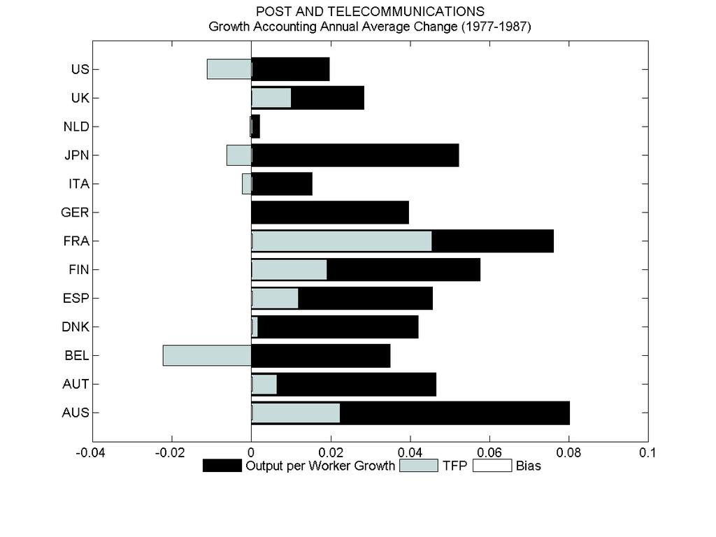
44 44 Figure 11: Post and Telecomunication Sector Growth Accounting

45 45 Figure 1: Chemicals and chemical Sector Growth Accounting