Interior Point Methods for Mathematical Programming

Size: px

Start display at page:

Download "Interior Point Methods for Mathematical Programming"

Merilyn Caldwell
5 years ago
Views:

1 Interior Point Methods for Mathematical Programming Clóvis C. Gonzaga Federal University of Santa Catarina, Florianópolis, Brazil EURO Roma

2 Our heroes Cauchy Newton Lagrange

3 Early results Unconstrained minimization minimize f (x) Inequality constraints minimize f (x) subject to g(x) 0 Cauchy (steepest descent): x + = x λ f (x) Newton: x + = x H(x) 1 f (x) For the constrained problem: Frisch, Fiacco, McCormick: F(x) = f (x) µ log( g i (x))

4 Early results Unconstrained minimization minimize f (x) Inequality constraints minimize f (x) subject to g(x) 0 Cauchy (steepest descent): x + = x λ f (x) Newton: x + = x H(x) 1 f (x) For the constrained problem: Frisch, Fiacco, McCormick: F(x) = f (x) µ log( g i (x))

5 Early results Unconstrained minimization minimize f (x) Inequality constraints minimize f (x) subject to g(x) 0 Cauchy (steepest descent): x + = x λ f (x) Newton: x + = x H(x) 1 f (x) For the constrained problem: Frisch, Fiacco, McCormick: F(x) = f (x) µ log( g i (x))

6 The barrier function Problem P1

7 Near the boundary, the barrier function tends to +.

8 The Linear Programming Problem Inequality constraints minimize c T x subject to Ax b Equality and non-negativity minimize subject to c T x Ax = b x 0 Interior point: x > 0. Solution: Ax = b. Feasible solution: Ax = b, x 0. Interior (feasible) solution: Ax = b, x > 0.

9 The Linear Programming Problem Inequality constraints minimize c T x subject to Ax b Equality and non-negativity minimize subject to c T x Ax = b x 0 Interior point: x > 0. Solution: Ax = b. Feasible solution: Ax = b, x 0. Interior (feasible) solution: Ax = b, x > 0.

10 The Linear Programming Problem Inequality constraints minimize c T x subject to Ax b Equality and non-negativity minimize subject to c T x Ax = b x 0 Interior point: x > 0. Solution: Ax = b. Feasible solution: Ax = b, x 0. Interior (feasible) solution: Ax = b, x > 0.

11 The Linear Programming Problem Inequality constraints minimize c T x subject to Ax b Equality and non-negativity minimize subject to c T x Ax = b x 0 Interior point: x > 0. Solution: Ax = b. Feasible solution: Ax = b, x 0. Interior (feasible) solution: Ax = b, x > 0.

12 Simplex Method: Dantzig 1948 Exponential in the worst case Good for usual problems.

13 Centers of gravity

22 Centers of gravity Conclusions Worst case performance: O(n ln(1/ε)) calls to the oracle.

23 Centers of gravity Conclusions Worst case performance: O(n ln(1/ε)) calls to the oracle. The method is generally not realizable: too difficult to compute the center of gravity. Work with simpler shapes: ellipsoids.

34 The ellipsoid method: Shor, Nemirovsky, Yudin, Khachyian Performance The computation of each new ellipsoid needs O(n 2 ) arithmetical operations. Worst case performance: O(n 2 ln(1/ε)) calls to the oracle, and O(n 4 ln(1/ε)) operations.

35 The Khachiyan Sputnik 1978 Khachiyan applied the ellipsoidal method to LP, and defined the number L=number of bits in the input for a problem with rational data. A solution with precision 2 L can be purified to an exact vertex solution of LP. Performance: O(n 4 )L computations.

37 Interior point methods Karmarkar 1984: projective IP method: O(n 3.5 L) computations. Renegar 1986: path following algorithm: O(n 3.5 L) computations. Vajdya and G. (independently) 1987: path following algorithms: O(n 3 L) computations.

38 Extensions Linear programming and quadratic programming: Jaceck Gonzio solved a Portfolio Optimization problem based on Markowitz analysis using 16 million scenarios, 1.10 billion variables, 353 million constraints in 53 iterations of an IP method in 50 minutes of a system of 1280 parallel processors. Second Order Cone Programming: extension of the Lorentz cone. Applications to Quadratically constrained quadratic programming, robust LP, robust Least Squares, Filter design, Portfolio Optimization, Truss design,... Semi-definite programming. A huge body of theory and applications to Structural Optimization, Optimal Control, Combinatorial Optimization,...

39 Extensions Linear programming and quadratic programming: Jaceck Gonzio solved a Portfolio Optimization problem based on Markowitz analysis using 16 million scenarios, 1.10 billion variables, 353 million constraints in 53 iterations of an IP method in 50 minutes of a system of 1280 parallel processors. Second Order Cone Programming: extension of the Lorentz cone. Applications to Quadratically constrained quadratic programming, robust LP, robust Least Squares, Filter design, Portfolio Optimization, Truss design,... Semi-definite programming. A huge body of theory and applications to Structural Optimization, Optimal Control, Combinatorial Optimization,...

40 Extensions Linear programming and quadratic programming: Jaceck Gonzio solved a Portfolio Optimization problem based on Markowitz analysis using 16 million scenarios, 1.10 billion variables, 353 million constraints in 53 iterations of an IP method in 50 minutes of a system of 1280 parallel processors. Second Order Cone Programming: extension of the Lorentz cone. Applications to Quadratically constrained quadratic programming, robust LP, robust Least Squares, Filter design, Portfolio Optimization, Truss design,... Semi-definite programming. A huge body of theory and applications to Structural Optimization, Optimal Control, Combinatorial Optimization,...

41 The Affine-Scaling direction Projection matrix Given c R n and a matrix A, c can be decomposed as c = P A c + A T y, where P A c N (A) is the projection of c into N (A).

42 The Affine-Scaling direction Linearly constrained problem: minimize subject to f (x) Ax = b x 0 Define c = f (x 0 ). The projected gradient (Cauchy) direction is c P = P A c, and the steepest descent direction is d = c P. It solves the trust region problem minimize{c T h Ah = 0, d }.

43 c c p h

44 Largest ball centered in xk

45 Largest simple ellipsoid centered in xk

46 The affine scaling direction c c p h

47 Largest ball centered in e = (1,1,...,1)

48 The Affine-Scaling direction Given a feasible point x 0, X = diag(x 0 ) and c = f (x 0 ) minimize subject to c T x Ax = b x 0 x = X x d = X d minimize subject to Scaled steepest descent direction: x = Xe (x is scaled into e): Dikin s direction: d = P AX Xc d = X d = XP AX Xc d = P AX Xc d = X d/ d. (Xc) T x AX x = b x 0

49 Dikin s algorithm Problem P1

50 Dikin s algorithm Problem P1

51 Dikin s algorithm Problem P1

52 Dikin s algorithm Problem P1

53 Affine scaling algorithm Problem P1

54 Affine scaling algorithm Problem P1

55 Affine scaling algorithm Problem P1

56 Affine scaling algorithm Problem P1

57 The logarithmic barrier function x R n ++ p(x) = Scaling: for a diagonal matrix D > 0 Derivatives: n i=1 logx i. p(dx) = p(x) + constant, p(dx) p(dy) = p(x) p(y). p(x) = x 1 p(e) = e 2 p(x) = X 2 2 p(e) = I. At x = e, the Hessian matrix is the identity, and hence the Newton direction coincides with the Cauchy direction.

58 The logarithmic barrier function x R n ++ p(x) = Scaling: for a diagonal matrix D > 0 Derivatives: n i=1 logx i. p(dx) = p(x) + constant, p(dx) p(dy) = p(x) p(y). p(x) = x 1 p(e) = e 2 p(x) = X 2 2 p(e) = I. At x = e, the Hessian matrix is the identity, and hence the Newton direction coincides with the Cauchy direction. At any x > 0, the affine scaling direction coincides with the Newton direction.

59 The penalized function in linear programming For x > 0, µ > 0 and α = 1/µ, minimize subject to f α (x) = αc T x + p(x) or f µ (x) = c T x + µp(x) c T x Ax = b x 0 minimize subject to c T x + µp(x) Ax = b x > 0 For α 0, f α is strictly convex and grows indefinitely near the boundary of the feasible set. Whenever the minimizers exist, they are defined uniquely by x α = argmin x Ω f α (x). In particular, if Ω is bounded, x 0 is the analytic center of Ω If the optimal face of the problem is bounded, then the curve α > 0 x α is well defined and is called the primal central path.

60 The penalized function in linear programming For x > 0, µ > 0 and α = 1/µ, minimize subject to f α (x) = αc T x + p(x) or f µ (x) = c T x + µp(x) c T x Ax = b x 0 minimize subject to c T x + µp(x) Ax = b x > 0 For α 0, f α is strictly convex and grows indefinitely near the boundary of the feasible set. Whenever the minimizers exist, they are defined uniquely by x α = argmin x Ω f α (x). In particular, if Ω is bounded, x 0 is the analytic center of Ω If the optimal face of the problem is bounded, then the curve α > 0 x α is well defined and is called the primal central path.

61 The penalized function in linear programming For x > 0, µ > 0 and α = 1/µ, minimize subject to f α (x) = αc T x + p(x) or f µ (x) = c T x + µp(x) c T x Ax = b x 0 minimize subject to c T x + µp(x) Ax = b x > 0 For α 0, f α is strictly convex and grows indefinitely near the boundary of the feasible set. Whenever the minimizers exist, they are defined uniquely by x α = argmin x Ω f α (x). In particular, if Ω is bounded, x 0 is the analytic center of Ω If the optimal face of the problem is bounded, then the curve α > 0 x α is well defined and is called the primal central path.

62 The central path Problem P1

63 Equivalent definitions of the central path There are four equivalent ways of defining central points: Minimizers of the penalized function: argmin x Ω f α (x). Analytic centers of constant cost slices argmin x Ω {p(x) c T x = K} Renegar centers: Analytic centers of Ω with an extra constraint c T x. argmin x Ω {p(x) log(k c T x) c T x < K} Primal-dual central points (seen ahead).

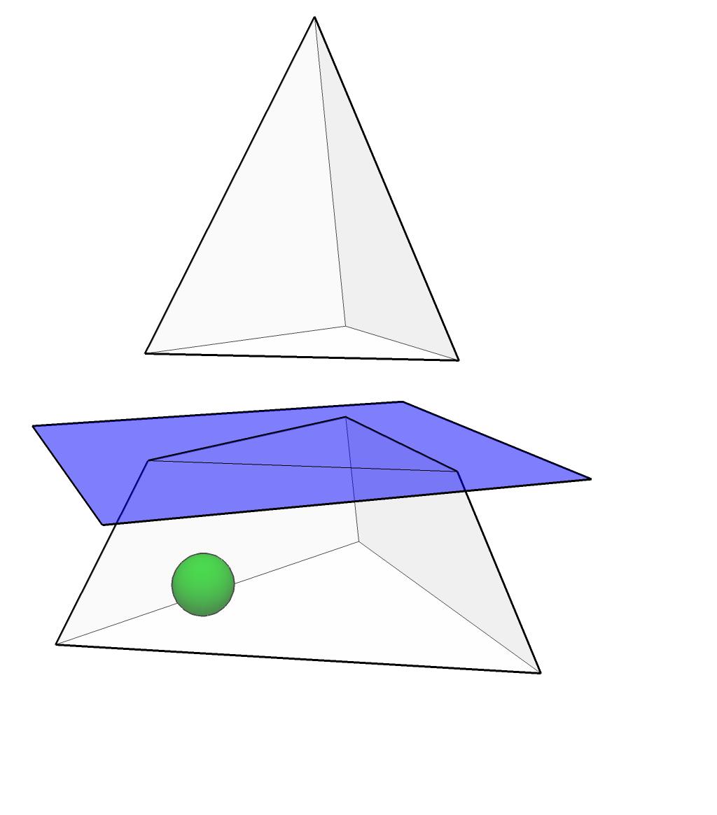
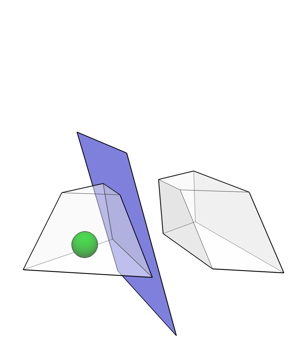
64 Constant cost slices Enter the new cut position (one point) and then the initial point

65 Constant cost slices Enter the new cut position (one point) and then the initial point

66 Constant cost slices Enter the new cut position (one point) and then the initial point

67 Renegar cuts Problem Ptemp

68 Renegar cuts Problem Ptemp

69 Renegar cuts Problem Ptemp

70 Renegar cuts Problem Ptemp

71 Renegar cuts Problem Ptemp

72 Renegar cuts Problem Ptemp

73 Centering The most important problem in interior point methods is the following: Centering problem Given a feasible interior point x 0 and a value α 0, solve approximately the problem minimize x Ω 0 αc T x + p(x). The Newton direction from x 0 coincides with the affine-scaling direction, and hence is the best possible. It is given by d = X d, d = P AX X(αc x 1 ) = αp AX Xc + P AX e.

74 Centering The most important problem in interior point methods is the following: Centering problem Given a feasible interior point x 0 and a value α 0, solve approximately the problem minimize x Ω 0 αc T x + p(x). The Newton direction from x 0 coincides with the affine-scaling direction, and hence is the best possible. It is given by d = X d, d = P AX X(αc x 1 ) = αp AX Xc + P AX e.

75 Efficiency of the Newton step for centering Newton direction: d = X d, d = P AX X(αc x 1 ) = αp AX Xc + P AX e. We define the Proximity to the central point as δ(x,α) = d = αp AX Xc + P AX e. The following important theorem says how efficient it is: Theorem Consider a feasible point x and a parameter α. Let x + = x + d be the point resulting from a Newton centering step. If δ(x,α) = δ < 1, then δ(x +,α) < δ 2. If δ(x,α) 0.5, then this value is a very good approximation to the euclidean distance between e and X 1 x α, i. e., between x and x α in the scaled space.

76 Efficiency of the Newton step for centering Newton direction: d = X d, d = P AX X(αc x 1 ) = αp AX Xc + P AX e. We define the Proximity to the central point as δ(x,α) = d = αp AX Xc + P AX e. The following important theorem says how efficient it is: Theorem Consider a feasible point x and a parameter α. Let x + = x + d be the point resulting from a Newton centering step. If δ(x,α) = δ < 1, then δ(x +,α) < δ 2. If δ(x,α) 0.5, then this value is a very good approximation to the euclidean distance between e and X 1 x α, i. e., between x and x α in the scaled space.

77 Short steps

78 Primal results as we saw are important to give a geometrical meaning to the procedures, and to develop the intuition. Also, these results can be generalized to a large class of problems, by generalizing the idea of barrier functions. From now on we shall deal with primal-dual results, which are more efficient for linear and non-linear programming.

79 The Linear Programming Problem LP LD minimize subject to c T x Ax = b x 0 maximize subject to b T y A T y c

80 The Linear Programming Problem LP LD minimize subject to c T x Ax = b x 0 maximize subject to b T y A T y + s = c s 0

81 The Linear Programming Problem LP minimize subject to KKT: multipliers y, s c T x Ax = b x 0 A T y + s = c Ax = b xs = 0 x,s 0 LD maximize subject to b T y A T y + s = c s 0

82 The Linear Programming Problem LP minimize subject to c T x Ax = b x 0 LD maximize subject to b T y A T y + s = c s 0 KKT: multipliers y, s A T y + s = c Ax = b xs = 0 x,s 0 KKT: multipliers x A T y + s = c Ax = b xs = 0 x,s 0

83 The Linear Programming Problem LP minimize subject to c T x Ax = b x 0 LD maximize subject to b T y A T y + s = c s 0 Primal-dual optimality A T y + s = c Ax = b xs = 0 x,s 0 Duality gap For x, y, s feasible, c T x b T y = x T s 0

84 The Linear Programming Problem LP minimize subject to c T x Ax = b x 0 LD maximize subject to b T y A T y + s = c s 0 Primal-dual optimality A T y + s = c Ax = b xs = 0 x,s 0 Duality gap For x, y, s feasible, c T x b T y = x T s 0 (LP) has solution x and (LD) has solution y,s if and only if the optimality conditions have solution x, y, s.

85 Primal-dual centering Let us write the KKT conditions for the centering problem (now using µ instead of α = 1/µ). minimize c T x µ logx i subject to Ax = b x > 0 Primal-dual center: KKT conditions xs = µe A T y + s = c Ax = b x,s > 0

86 Primal-dual centering Let us write the KKT conditions for the centering problem (now using µ instead of α = 1/µ). minimize c T x µ logx i subject to Ax = b x > 0 Primal-dual center: KKT conditions xs = µe A T y + s = c Ax = b x,s > 0

87 Generalization Let us write the KKT conditions for the convex quadratic programming problem minimize subject to c T x xt Hx Ax = b x > 0 The first KKT condition is written as c + Hx A T y s = 0 To obtain a symmetrical formulation for the problem, we may multiply this equation by a matrix B whose rows form a basis for the null space of A. Then BA T y = 0, and we obtain the following conditions conditions: xs = 0 BHx + Bs = Bc Ax = b x,s 0

88 Horizontal linear complementarity problem In any case, the problem can be written as xs = 0 Qx + Rs = b x,s 0 This is a linear complementarity problem, which includes linear and quadratic programming as particular problems. The techniques studied here apply to these problems, as long as the following monotonicity condition holds: For any feasible pair of directions (u,v) such that Qu + Rv = 0, we have u T v 0. The optimal face: the optimal solutions must satisfy x i s i = 0 for i = 1,...,n. This is a combinatorial constraint, responsible for all the difficulty in the solution.

89 Horizontal linear complementarity problem In any case, the problem can be written as xs = 0 Qx + Rs = b x,s 0 This is a linear complementarity problem, which includes linear and quadratic programming as particular problems. The techniques studied here apply to these problems, as long as the following monotonicity condition holds: For any feasible pair of directions (u,v) such that Qu + Rv = 0, we have u T v 0. The optimal face: the optimal solutions must satisfy x i s i = 0 for i = 1,...,n. This is a combinatorial constraint, responsible for all the difficulty in the solution.

90 Primal-dual centering: the Newton step Given x,s feasible and µ > 0, find x + = x + u s + = s + v such that x + s + = µe Qx + + Rs + = b xs + su + xv + uv = µe Qu + Rv = 0 Newton step Xv + Su = xs + µe Qu + Rv = 0 Solving this linear system is all the work. In the case of linear programming one should keep the multipliers y and simplify the resulting system of equations

91 Primal-dual centering: the Newton step Given x,s feasible and µ > 0, find x + = x + u s + = s + v such that x + s + = µe Qx + + Rs + = b xs + su + xv + uv = µe Qu + Rv = 0 Newton step Xv + Su = xs + µe Qu + Rv = 0 Solving this linear system is all the work. In the case of linear programming one should keep the multipliers y and simplify the resulting system of equations

92 Primal-dual centering: the Newton step Given x,s feasible and µ > 0, find x + = x + u s + = s + v such that x + s + = µe Qx + + Rs + = b xs + su + xv + uv = µe Qu + Rv = 0 Newton step Xv + Su = xs + µe Qu + Rv = 0 Solving this linear system is all the work. In the case of linear programming one should keep the multipliers y and simplify the resulting system of equations

93 Primal-dual centering: Proximity measure Given x,s feasible and µ > 0, we want xs = µe or equivalently xs µ e = 0 The actual error in this equation gives the proximity measure: Proximity measure Theorem x,s,µ δ(x,s,µ) = xs µ e. Given a feasible pair (x,s) and a parameter µ, Let x + = x + u and s + = s + v be the point resulting from a Newton centering step. If δ(x,s,µ) = δ < 1, then δ(x +,s +,µ) < 1 8 δ 2 1 δ. In particular, if δ 0.7, then δ(x +,s +,µ) < δ 2.

94 Primal-dual centering: Proximity measure Given x,s feasible and µ > 0, we want xs = µe or equivalently xs µ e = 0 The actual error in this equation gives the proximity measure: Proximity measure Theorem x,s,µ δ(x,s,µ) = xs µ e. Given a feasible pair (x,s) and a parameter µ, Let x + = x + u and s + = s + v be the point resulting from a Newton centering step. If δ(x,s,µ) = δ < 1, then δ(x +,s +,µ) < 1 8 δ 2 1 δ. In particular, if δ 0.7, then δ(x +,s +,µ) < δ 2.

95 Primal-dual path following: Traditional approach Assume that we have x,s,µ such that (x,s) is feasible and δ(x,s,µ) α < 1 Choose µ + = γµ, with γ < 1. Use Newton s algorithm (with line searches to avoid infeasible points) to find (x +,s + ) such that δ(x +,s +,µ + ) α Neighborhood of the central path Given β (0,1), we define the neighborhood η(α) as the set of all feasible pairs (x,s) such that for some µ > 0 δ(x,s,µ) β The methods must ensure that all points are in such a neighborhood, using line searches

96 Primal-dual path following: Traditional approach Assume that we have x,s,µ such that (x,s) is feasible and δ(x,s,µ) α < 1 Choose µ + = γµ, with γ < 1. Use Newton s algorithm (with line searches to avoid infeasible points) to find (x +,s + ) such that δ(x +,s +,µ + ) α Neighborhood of the central path Given β (0,1), we define the neighborhood η(α) as the set of all feasible pairs (x,s) such that for some µ > 0 δ(x,s,µ) β The methods must ensure that all points are in such a neighborhood, using line searches

97 Primal-dual path following: Traditional approach Assume that we have x,s,µ such that (x,s) is feasible and δ(x,s,µ) α < 1 Choose µ + = γµ, with γ < 1. Use Newton s algorithm (with line searches to avoid infeasible points) to find (x +,s + ) such that δ(x +,s +,µ + ) α Neighborhood of the central path Given β (0,1), we define the neighborhood η(α) as the set of all feasible pairs (x,s) such that for some µ > 0 δ(x,s,µ) β The methods must ensure that all points are in such a neighborhood, using line searches

98 A neighborhood of the central path

99 Short steps Using γ near 1, we obtain short steps. With γ = 0.4/ n, only one Newton step is needed at each iteration, and the algorithm is polynomial: it finds a solution with precision 2 L in O( nl) iterations.

100 Short steps Problem P1

101 Large steps Using γ small, say γ = 0.1, we obtain large steps. This uses to work well in practice, but some sort of line search is needed, to avoid leaving the neighborhood. Predictor-corrector methods are better, as we shall see.

102 Large steps Problem P1

103 Adaptive methods Assume that (x,s) feasible is given in η(β), but no value of µ is given. Then we know: if (x,s) is a central point, then xs = µe implies x T s = nµ. Hence the best choice for µ is µ = x T s/n. If (x,s) is not a central point, the value µ(x,s) = x T s/n gives a parameter value which in a certain sense is the best possible. An adaptive algorithm does not use a value of µ coming from a former iteration: it computes µ(x, s) and then chooses a value γµ(x, s) as new target. The target may be far. Compute a direction (u,v) and follow it until δ(x + λu,s + λv,µ(x + λu,s + λv)) = β

104 Adaptive steps

105 Predictor-corrector methods Alternate two kinds of iterations: Predictor: An iteration starts with (x, s) near the central path, and computes a Newton step (u, v) with goal γµ(x, s), γ small. Follow it until δ(x + λu,s + λv,µ(x + λu,s + λv)) = β Corrector: Set x + = x + λu, s + = s + λv, compute µ = µ(x +,s + ) and take a Newton step with target µ If the predictor uses γ = 0, it is called the affine scaling step. It has no centering, and tries to solve the original problem in one step. Using a neighborhood with β = 0.5, the resulting algorithm (the Mizuno-Todd-Ye algorithm) converges quadratically to an optimal solution, keeping the complexity at its best value of O( nl) iterations.

106 Predictor-corrector methods Alternate two kinds of iterations: Predictor: An iteration starts with (x, s) near the central path, and computes a Newton step (u, v) with goal γµ(x, s), γ small. Follow it until δ(x + λu,s + λv,µ(x + λu,s + λv)) = β Corrector: Set x + = x + λu, s + = s + λv, compute µ = µ(x +,s + ) and take a Newton step with target µ If the predictor uses γ = 0, it is called the affine scaling step. It has no centering, and tries to solve the original problem in one step. Using a neighborhood with β = 0.5, the resulting algorithm (the Mizuno-Todd-Ye algorithm) converges quadratically to an optimal solution, keeping the complexity at its best value of O( nl) iterations.

107 Predictor-corrector

108 Mehrotra Predictor-corrector method: second order When computing the Newton step, we eliminated the nonlinear term uv in the equation xs + su + xv + uv = µe Qu + Rv = 0 The second order method corrects the values of u,v by estimating the value of the term uv by a predictor step. Predictor: An iteration starts with (x, s) near the central path, and computes a Newton step (u,v) with goal µ +, small. The first equation is Compute a correction ( u, v) by xv + su = xs + µ + e x v + s u = uv. Line search: Set x + = x + λu + λ 2 u, s + = s + λv + λ 2 v, by a line search so that δ(x +,s +,µ(x +,s + )) = β.

109 Mehrotra Predictor-corrector

110 Thank you

Interior Point Methods in Mathematical Programming

Interior Point Methods in Mathematical Programming Clóvis C. Gonzaga Federal University of Santa Catarina, Brazil Journées en l honneur de Pierre Huard Paris, novembre 2008 01 00 11 00 000 000 000 000