Signals and Systems Chapter 2

Size: px

Start display at page:

Download "Signals and Systems Chapter 2"

Maximillian Logan
5 years ago
Views:

1 Signals and Systems Chapter 2 Continuous-Time Systems Prof. Yasser Mostafa Kadah

2 Overview of Chapter 2 Systems and their classification Linear time-invariant systems

3 System Concept Mathematical transformation of an input signal (or signals) into an output signal (or signals) Idealized model of the physical device or process Examples: Electrical/electronic circuits In practice, the model and the mathematical representation are not unique

4 System Classification Static or dynamic systems Capability of storing energy, or remembering state Lumped- or distributed-parameter systems Passive or active systems Ex: circuits elements Continuous time, discrete time, digital, or hybrid systems According to type of input/output signals

5 LTI Continuous-Time Systems A continuous-time system is a system in which the signals at its input and output are continuous-time signals

6 Linearity A linear system is a system in which the superposition holds Output Scaling Additivity Linear System input Output Nonlinear System Examples: y(x)= a x y(x)= a x + b Linear Nonlinear input

7 Linearity Examples Show that the following systems are nonlinear: where x(t) is the input and y(t), z(t), and v(t) are the outputs. Whenever the explicit relation between the input and the output of a system is represented by a nonlinear expression the system is nonlinear

8 Linearity Examples Consider each of the components of an RLC circuit and determine under what conditions they are linear. R C L

9 Linearity Examples Op Amp Linear or nonlinear region Virtual short

10 Time Invariance System S does not change with time System does not age its parameters are constant Example: AM modulation

11 RLC Circuits Kirchhoff s voltage law, d/dt Second-order differential equation with constant coefficients Input the voltage source v(t) Output the current i(t)

12 Representation of Systems by Differential Equations Given a dynamic system represented by a linear differential equation with constant coefficients: N initial conditions: Input x(t)=0 for t < 0, Complete response y(t) for t>=0 has two parts: Zero-state response Zero-input response

13 Representation of Systems by Differential Equations Linear Time-Invariant Systems System represented by linear differential equation with constant coefficients Initial conditions are all zero Output depends exclusively on input only Nonlinear Systems Nonzero initial conditions means nonlinearity Can also be time-varying

14 Representation of Systems by Differential Equations Define derivative operator D as, Then,

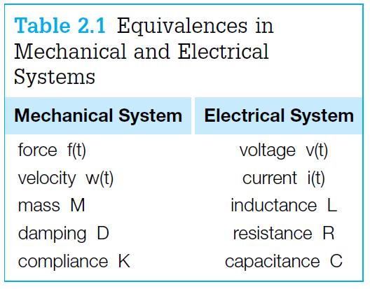
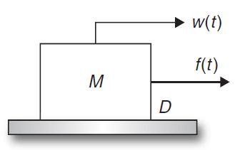
15 Analog Mechanical Systems

16 Application of Superposition and Time Invariance The computation of the output of an LTI system is simplified when the input can be represented as the combination of signals for which we know their response. Using superposition and time invariance properties

17 Application of Superposition and Time Invariance: Example Example 1: Given the response of an RL circuit to a unitstep source u(t), find the response to a pulse

impulse (t) as input, and zero initial conditions The response of an LTI system S

18 Convolution Integral Generic representation of a signal: The impulse response of an analog LTI system, h(t), is the output of the system corresponding to an impulse (t) as input, and zero initial conditions The response of an LTI system S represented by its impulse response h(t) to any signal x(t) is given by: Convolution Integral

19 Convolution Integral: Observations Impulse response is fundamental in the characterization of linear time-invariant systems Any system characterized by the convolution integral is linear and time invariant by the above construction The convolution integral is a general representation of LTI systems, given that it was obtained from a generic representation of the input signal Given that a system represented by a linear differential equation with constant coefficients and no initial conditions, or input, before t=0 is LTI, one should be able to represent that system by a convolution integral after finding its impulse response h(t)

20 Convolution Integral: Example Example: Obtain the impulse response of a capacitor and use it to find its unit-step response by means of the convolution integral. Let C = 1 F.

21 Causality A continuous-time system S is called causal if: Whenever the input x(t)=0 and there are no initial conditions, the output is y(t)=0 The output y(t) does not depend on future inputs For a value > 0, when considering causality it is helpful to think of: Time t (the time at which the output y(t) is being computed) as the present Times t- as the past Times t+ as the future

22 Causality

23 Graphical Computation of Convolution Integral Example 1: Graphically find the unit-step y(t) response of an averager, with T=1 sec, which has an impulse response h(t)= u(t)-u(t-1)

24 Graphical Computation of Convolution Integral Example 2: Consider the graphical computation of the convolution integral of two pulses of the same duration

25 Interconnection of Systems Block Diagrams (a) Cascade (commutative) (b) Parallel (distributive) (c) Feedback

26 Bounded-Input Bounded-Output Stability (BIBO) For a bounded (i.e., well-behaved) input x(t), the output of a BIBO stable system y(t) is also bounded An LTI system with an absolutely integrable impulse response is BIBO stable Example: Multi-echo path system

27 Problem Assignments Problems: 2.3, 2.4, 2.8, 2.9, 2.10, 2.12, 2.14 Partial Solutions available from the student section of the textbook web site

Therefore the new Fourier coefficients are. Module 2 : Signals in Frequency Domain Problem Set 2. Problem 1

Therefore the new Fourier coefficients are. Module 2 : Signals in Frequency Domain Problem Set 2. Problem 1 Module 2 : Signals in Frequency Domain Problem Set 2 Problem 1 Let be a periodic signal with fundamental period T and Fourier series coefficients. Derive the Fourier series coefficients of each of the