Lecture 8 CORRELATION AND LINEAR REGRESSION
|
|
|
- Cleopatra Jones
- 5 years ago
- Views:
Transcription

1 Announcements CBA5 open in exam mode - deadline midnight Friday! Question 2 on this week s exercises is a prize question. The first good attempt handed in to me by 12 midday this Friday will merit a prize...
2 Assignment 2 The Minitab-based Assignment 2 which would have been set if there had been no disruption has been scrapped, and the material on Minitab is non-examinable. A revised assignment 2 is due to be set. Proposed deadline is Friday May 4th, 1pm, subject to confirmation (it won t be before that!)
3 Lecture 8 CORRELATION AND LINEAR REGRESSION
4 Introduction In this lecture we look at relationships between pairs of continuous variables. These might be
5 Introduction In this lecture we look at relationships between pairs of continuous variables. These might be height and weight
6 Introduction In this lecture we look at relationships between pairs of continuous variables. These might be height and weight market value and number of transactions
7 Introduction In this lecture we look at relationships between pairs of continuous variables. These might be height and weight market value and number of transactions temperatures and sales of ice cream
8 Introduction In this lecture we look at relationships between pairs of continuous variables. These might be height and weight market value and number of transactions temperatures and sales of ice cream We can examine the relationship between our two variables through a scatter diagram (plot one against the other).
9 Introduction In this lecture we look at relationships between pairs of continuous variables. These might be height and weight market value and number of transactions temperatures and sales of ice cream We can examine the relationship between our two variables through a scatter diagram (plot one against the other). Today we will look at how to examine such relationships more formally.

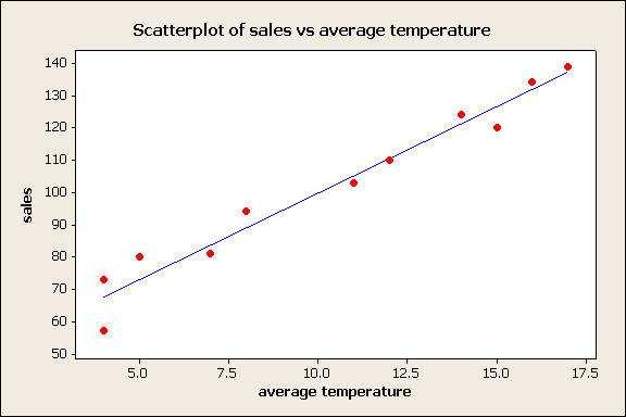
10 Example: ice cream sales The following data are monthly ice cream sales at Luigi Minchella s ice cream parlour.
11 Month Average Temp ( o C) Sales ( 000 s) January 4 73 February 4 57 March 7 81 April 8 94 May June July August September October November 7 81 December 5 80
12 Month Average Temp ( o C) Sales ( 000 s) January 4 73 February 4 57 March 7 81 April 8 94 May June July August September October November 7 81 December 5 80 Is there any relationship between temperature and sales?
13 Month Average Temp ( o C) Sales ( 000 s) January 4 73 February 4 57 March 7 81 April 8 94 May June July August September October November 7 81 December 5 80 Is there any relationship between temperature and sales? Can you DESCRIBE this relationship?
14
15 The scatter plot goes uphill, so we say there is a positive relationship between temperature and ice cream sales.
16 The scatter plot goes uphill, so we say there is a positive relationship between temperature and ice cream sales. As temperatures rise, so do ice cream sales!
17 The scatter plot goes uphill, so we say there is a positive relationship between temperature and ice cream sales. As temperatures rise, so do ice cream sales! If the scatter plot had shown a downhill slope, we would have a negative relationship.
18 The scatter plot goes uphill, so we say there is a positive relationship between temperature and ice cream sales. As temperatures rise, so do ice cream sales! If the scatter plot had shown a downhill slope, we would have a negative relationship. We could draw a straight line through the middle of most of the points. Thus, there is also a linear association present.
19 The scatter plot goes uphill, so we say there is a positive relationship between temperature and ice cream sales. As temperatures rise, so do ice cream sales! If the scatter plot had shown a downhill slope, we would have a negative relationship. We could draw a straight line through the middle of most of the points. Thus, there is also a linear association present. If we were to draw a line through the points, most points would lie close to this line. The closer the points lie to a line, the stronger the relationship.
20 Correlation We now look at how to quantify the relationship between two variables by calculating the sample correlation coefficient. This is
21 Correlation We now look at how to quantify the relationship between two variables by calculating the sample correlation coefficient. This is r = S XY SXX S YY, where
22 Correlation We now look at how to quantify the relationship between two variables by calculating the sample correlation coefficient. This is r = S XY SXX S YY, where S XY = ( xy ) n xȳ,
23 Correlation We now look at how to quantify the relationship between two variables by calculating the sample correlation coefficient. This is r = S XY SXX S YY, where S XY = S XX = ( ) xy n xȳ, ( ) x 2 n x 2,
24 Correlation We now look at how to quantify the relationship between two variables by calculating the sample correlation coefficient. This is r = S XY SXX S YY, where S XY = S XX = S YY = ( ) xy n xȳ, ( ) x 2 n x 2, ( ) y 2 nȳ 2.
25 r always lies between 1 and +1.
26 r always lies between 1 and +1. If r is close to +1, we have evidence of a strong positive (linear) association.
27 r always lies between 1 and +1. If r is close to +1, we have evidence of a strong positive (linear) association. If r is close to 1, we have evidence of a strong negative (linear) association.
28 r always lies between 1 and +1. If r is close to +1, we have evidence of a strong positive (linear) association. If r is close to 1, we have evidence of a strong negative (linear) association. If r is close to zero, there is probably no association!
29 r always lies between 1 and +1. If r is close to +1, we have evidence of a strong positive (linear) association. If r is close to 1, we have evidence of a strong negative (linear) association. If r is close to zero, there is probably no association! A correlation coefficient close to zero does not imply no relationship at all, just no linear relationship.
30 Example: ice cream sales The easiest way to calculate r is to draw up a table!
31 Example: ice cream sales The easiest way to calculate r is to draw up a table! Ü Ý Ü 2 Ý 2 ÜÝ 4 73
32 Example: ice cream sales The easiest way to calculate r is to draw up a table! Ü Ý Ü 2 Ý 2 ÜÝ
33 Example: ice cream sales The easiest way to calculate r is to draw up a table! Ü Ý Ü 2 Ý 2 ÜÝ
34 Example: ice cream sales The easiest way to calculate r is to draw up a table! Ü Ý Ü 2 Ý 2 ÜÝ
35 Example: ice cream sales The easiest way to calculate r is to draw up a table! Ü Ý Ü 2 Ý 2 ÜÝ
36 Example: ice cream sales The easiest way to calculate r is to draw up a table! Ü Ý Ü 2 Ý 2 ÜÝ
37 Example: ice cream sales The easiest way to calculate r is to draw up a table! Ü Ý Ü 2 Ý 2 ÜÝ
38 Example: ice cream sales The easiest way to calculate r is to draw up a table! Ü Ý Ü 2 Ý 2 ÜÝ
39 Example: ice cream sales The easiest way to calculate r is to draw up a table! Ü Ý Ü 2 Ý 2 ÜÝ
40 Example: ice cream sales The easiest way to calculate r is to draw up a table! Ü Ý Ü 2 Ý 2 ÜÝ
41 Notice in the formulae for S XY, S XX and S YY we need the sample means x and ȳ. Thus,
42 Notice in the formulae for S XY, S XX and S YY we need the sample means x and ȳ. Thus, x = = 10 and
43 Notice in the formulae for S XY, S XX and S YY we need the sample means x and ȳ. Thus, x = = 10 and ȳ = = 100.
44 Similarly,
45 Similarly, S XY = ( xy ) n xȳ = = 1362,
46 Similarly, S XY = ( xy ) n xȳ = = 1362, ( ) S XX = x 2 n x 2 = = 250 and
47 Similarly, S XY = ( xy ) n xȳ = = 1362, ( ) S XX = x 2 n x 2 = = 250 and ( ) S YY = y 2 nȳ 2 = = 7674.
48 Thus,
49 Thus, r = S XY SXX S YY
50 Thus, r = = S XY SXX S YY
51 Thus, r = = S XY SXX S YY = (to 3 decimal places).
52 A few points to remember...
53 A few points to remember... If your calculated correlation coefficient does not lie between 1 and +1, you ve done something wrong!
54 A few points to remember... If your calculated correlation coefficient does not lie between 1 and +1, you ve done something wrong! Check that your correlation coefficient agrees with your plot
55 A few points to remember... If your calculated correlation coefficient does not lie between 1 and +1, you ve done something wrong! Check that your correlation coefficient agrees with your plot an uphill slope ties in with a positive correlation coefficient;
56 A few points to remember... If your calculated correlation coefficient does not lie between 1 and +1, you ve done something wrong! Check that your correlation coefficient agrees with your plot an uphill slope ties in with a positive correlation coefficient; a downhill slope ties in with a negative correlation coefficient;
57 A few points to remember... If your calculated correlation coefficient does not lie between 1 and +1, you ve done something wrong! Check that your correlation coefficient agrees with your plot an uphill slope ties in with a positive correlation coefficient; a downhill slope ties in with a negative correlation coefficient; a random scattering of points indicates a correlation coefficient close to zero;
58 A few points to remember... If your calculated correlation coefficient does not lie between 1 and +1, you ve done something wrong! Check that your correlation coefficient agrees with your plot an uphill slope ties in with a positive correlation coefficient; a downhill slope ties in with a negative correlation coefficient; a random scattering of points indicates a correlation coefficient close to zero; the closer the points lie to a straight line (either uphill or downhill ), the closer to either +1 or 1 the correlation coefficient will be!
59 Simple linear regression A correlation analysis helps to establish whether or not there is a linear relationship between two variables. However, it doesn t allow us to use this linear relationship.
60 Simple linear regression A correlation analysis helps to establish whether or not there is a linear relationship between two variables. However, it doesn t allow us to use this linear relationship. Regression analysis allows us to use the linear relationship between two variables. For example, with a regression analysis, we can predict the value of one variable given the value of another.
61 Simple linear regression A correlation analysis helps to establish whether or not there is a linear relationship between two variables. However, it doesn t allow us to use this linear relationship. Regression analysis allows us to use the linear relationship between two variables. For example, with a regression analysis, we can predict the value of one variable given the value of another. To perform a regression analysis, we must assume that
62 Simple linear regression A correlation analysis helps to establish whether or not there is a linear relationship between two variables. However, it doesn t allow us to use this linear relationship. Regression analysis allows us to use the linear relationship between two variables. For example, with a regression analysis, we can predict the value of one variable given the value of another. To perform a regression analysis, we must assume that the scatter plot of the two variables (roughly) shows a straight line, and
63 Simple linear regression A correlation analysis helps to establish whether or not there is a linear relationship between two variables. However, it doesn t allow us to use this linear relationship. Regression analysis allows us to use the linear relationship between two variables. For example, with a regression analysis, we can predict the value of one variable given the value of another. To perform a regression analysis, we must assume that the scatter plot of the two variables (roughly) shows a straight line, and the spread in the Y direction is roughly constant with X.
64
65 Look at the scatter plot of ice cream sales against temperature.
66 Look at the scatter plot of ice cream sales against temperature. A line of best fit can be drawn through the data;
67 Look at the scatter plot of ice cream sales against temperature. A line of best fit can be drawn through the data; This line could then be used to make predictions of ice cream sales based on temperature.
68 Look at the scatter plot of ice cream sales against temperature. A line of best fit can be drawn through the data; This line could then be used to make predictions of ice cream sales based on temperature. However, everyone s line is bound to be slightly different!
69 Look at the scatter plot of ice cream sales against temperature. A line of best fit can be drawn through the data; This line could then be used to make predictions of ice cream sales based on temperature. However, everyone s line is bound to be slightly different! And so everyone s predictions will be slightly different!
70 Look at the scatter plot of ice cream sales against temperature. A line of best fit can be drawn through the data; This line could then be used to make predictions of ice cream sales based on temperature. However, everyone s line is bound to be slightly different! And so everyone s predictions will be slightly different! The aim of regression analysis is to find the best line which goes through the data.
71 Look at the scatter plot of ice cream sales against temperature. A line of best fit can be drawn through the data; This line could then be used to make predictions of ice cream sales based on temperature. However, everyone s line is bound to be slightly different! And so everyone s predictions will be slightly different! The aim of regression analysis is to find the best line which goes through the data. At this point, we should remind ourselves about the equation for a straight line and how to draw it!
72 The regression equation
73 The regression equation The simple linear regression model is given by Y = α+βx +ǫ, where
74 The regression equation The simple linear regression model is given by Y = α+βx +ǫ, where Y is the response variable and
75 The regression equation The simple linear regression model is given by Y = α+βx +ǫ, where Y is the response variable and X is the explanatory variable.
76 The regression equation The simple linear regression model is given by where Y = α+βx +ǫ, Y is the response variable and X is the explanatory variable. ǫ is the random error taken to be zero on average, with constant variance.
77 The regression equation The simple linear regression model is given by where Y = α+βx +ǫ, Y is the response variable and X is the explanatory variable. ǫ is the random error taken to be zero on average, with constant variance. α represents the intercept of the regression line (the point where the line cuts the Y axis),
78 The regression equation The simple linear regression model is given by where Y = α+βx +ǫ, Y is the response variable and X is the explanatory variable. ǫ is the random error taken to be zero on average, with constant variance. α represents the intercept of the regression line (the point where the line cuts the Y axis), β represents the slope of the regression line (i.e. how steep the line is), and
79 The regression equation The simple linear regression model is given by where Y = α+βx +ǫ, Y is the response variable and X is the explanatory variable. ǫ is the random error taken to be zero on average, with constant variance. α represents the intercept of the regression line (the point where the line cuts the Y axis), β represents the slope of the regression line (i.e. how steep the line is), and We need to estimate α and β from our sample data. But how?
80 Remember, the aim of regression analysis is to find a line which goes through the middle of the data in the scatter plot, closer to the points than any other line;
81 Remember, the aim of regression analysis is to find a line which goes through the middle of the data in the scatter plot, closer to the points than any other line; So the best line will minimise any gaps between the line and the data!
82 Remember, the aim of regression analysis is to find a line which goes through the middle of the data in the scatter plot, closer to the points than any other line; So the best line will minimise any gaps between the line and the data! It turns out that the values of α and β which give this best line are ˆβ = S XY S XX and
83 Remember, the aim of regression analysis is to find a line which goes through the middle of the data in the scatter plot, closer to the points than any other line; So the best line will minimise any gaps between the line and the data! It turns out that the values of α and β which give this best line are ˆβ = S XY S XX and ˆα = ȳ ˆβ x.
84 Example: ice cream sales For the ice cream sales data, we can find the best line using the formulae on the previous slide! Thus
85 Example: ice cream sales For the ice cream sales data, we can find the best line using the formulae on the previous slide! Thus and ˆβ = S XY S XX = = 5.448,
86 Example: ice cream sales For the ice cream sales data, we can find the best line using the formulae on the previous slide! Thus and ˆβ = S XY S XX = = 5.448, ˆα = ȳ ˆβ x = =
87 Thus, the regression equation is
88 Thus, the regression equation is Ý = Ü
89
90 Making predictions We can use our estimated regression equation to make predictions of ice cream sales based on average temperature.
91 For example: Predict monthly sales if the average temperature is 10 o C.
92 For example: Predict monthly sales if the average temperature is 10 o C. We can use take a reading from our graph, or, more accurately, use our regression equation! y = x = = = 100, i.e.
93 For example: Predict monthly sales if the average temperature is 10 o C. We can use take a reading from our graph, or, more accurately, use our regression equation! y = x = = = 100, i.e. if the average temperature is 10 o C, we can expect sales of 100,000. i.e.
Time Series and Forecasting
 Chapter 8 Time Series and Forecasting 8.1 Introduction A time series is a collection of observations made sequentially in time. When observations are made continuously, the time series is said to be continuous;
Midterm 2 - Solutions
 Ecn 102 - Analysis of Economic Data University of California - Davis February 24, 2010 Instructor: John Parman Midterm 2 - Solutions You have until 10:20am to complete this exam. Please remember to put
ACE2013: Statistics for Marketing and Management
 ACE2013: Statistics for Marketing and Management Semester 2: 2013 14 Formalities Welcome to ACE2013: Part 2 Welcome! I ve decided to call this part of the course Statistical Business Modelling from now
Psych 10 / Stats 60, Practice Problem Set 10 (Week 10 Material), Solutions
, Solutions") Psych 10 / Stats 60, Practice Problem Set 10 (Week 10 Material), Solutions Part 1: Conceptual ideas about correlation and regression Tintle 10.1.1 The association would be negative (as distance increases,
Psych 10 / Stats 60, Practice Problem Set 10 (Week 10 Material), Solutions Part 1: Conceptual ideas about correlation and regression Tintle 10.1.1 The association would be negative (as distance increases,
Regression Analysis II
 Regression Analysis II Measures of Goodness of fit Two measures of Goodness of fit Measure of the absolute fit of the sample points to the sample regression line Standard error of the estimate An index
A Plot of the Tracking Signals Calculated in Exhibit 3.9
 CHAPTER 3 FORECASTING 1 Measurement of Error We can get a better feel for what the MAD and tracking signal mean by plotting the points on a graph. Though this is not completely legitimate from a sample-size
AMS 315/576 Lecture Notes. Chapter 11. Simple Linear Regression
 AMS 315/576 Lecture Notes Chapter 11. Simple Linear Regression 11.1 Motivation A restaurant opening on a reservations-only basis would like to use the number of advance reservations x to predict the number
MAT2377. Rafa l Kulik. Version 2015/November/26. Rafa l Kulik
 MAT2377 Rafa l Kulik Version 2015/November/26 Rafa l Kulik Bivariate data and scatterplot Data: Hydrocarbon level (x) and Oxygen level (y): x: 0.99, 1.02, 1.15, 1.29, 1.46, 1.36, 0.87, 1.23, 1.55, 1.40,
Week Topics of study Home/Independent Learning Assessment (If in addition to homework) 7 th September 2015
 7 th September 2015") Week Topics of study Home/Independent Learning Assessment (If in addition to homework) 7 th September Functions: define the terms range and domain (PLC 1A) and identify the range and domain of given functions
Week Topics of study Home/Independent Learning Assessment (If in addition to homework) 7 th September Functions: define the terms range and domain (PLC 1A) and identify the range and domain of given functions
6-1 Slope. Objectives 1. find the slope of a line 2. use rate of change to solve problems
 6-1 Slope Objectives 1. find the slope of a line 2. use rate of change to solve problems What is the meaning of this sign? 1. Icy Road Ahead 2. Steep Road Ahead 3. Curvy Road Ahead 4. Trucks Entering Highway
Chapter 1 0+7= 1+6= 2+5= 3+4= 4+3= 5+2= 6+1= 7+0= How would you write five plus two equals seven?
 Chapter 1 0+7= 1+6= 2+5= 3+4= 4+3= 5+2= 6+1= 7+0= If 3 cats plus 4 cats is 7 cats, what does 4 olives plus 3 olives equal? olives How would you write five plus two equals seven? Chapter 2 Tom has 4 apples
Chapter 12 - Part I: Correlation Analysis
 ST coursework due Friday, April - Chapter - Part I: Correlation Analysis Textbook Assignment Page - # Page - #, Page - # Lab Assignment # (available on ST webpage) GOALS When you have completed this lecture,
Section Linear Correlation and Regression. Copyright 2013, 2010, 2007, Pearson, Education, Inc.
 Section 13.7 Linear Correlation and Regression What You Will Learn Linear Correlation Scatter Diagram Linear Regression Least Squares Line 13.7-2 Linear Correlation Linear correlation is used to determine
Product and Inventory Management (35E00300) Forecasting Models Trend analysis
 Forecasting Models Trend analysis") Product and Inventory Management (35E00300) Forecasting Models Trend analysis Exponential Smoothing Data Storage Shed Sales Period Actual Value(Y t ) Ŷ t-1 α Y t-1 Ŷ t-1 Ŷ t January 10 = 10 0.1 February
Product and Inventory Management (35E00300) Forecasting Models Trend analysis Exponential Smoothing Data Storage Shed Sales Period Actual Value(Y t ) Ŷ t-1 α Y t-1 Ŷ t-1 Ŷ t January 10 = 10 0.1 February
Chapter 12 - Lecture 2 Inferences about regression coefficient
 Chapter 12 - Lecture 2 Inferences about regression coefficient April 19th, 2010 Facts about slope Test Statistic Confidence interval Hypothesis testing Test using ANOVA Table Facts about slope In previous
Announcements. J. Parman (UC-Davis) Analysis of Economic Data, Winter 2011 February 8, / 45
 Analysis of Economic Data, Winter 2011 February 8, / 45") Announcements Solutions to Problem Set 3 are posted Problem Set 4 is posted, It will be graded and is due a week from Friday You already know everything you need to work on Problem Set 4 Professor Miller
Announcements Solutions to Problem Set 3 are posted Problem Set 4 is posted, It will be graded and is due a week from Friday You already know everything you need to work on Problem Set 4 Professor Miller
CORRELATION AND REGRESSION
 CORRELATION AND REGRESSION CORRELATION The correlation coefficient is a number, between -1 and +1, which measures the strength of the relationship between two sets of data. The closer the correlation coefficient
Chapter 6: Exploring Data: Relationships Lesson Plan
 Chapter 6: Exploring Data: Relationships Lesson Plan For All Practical Purposes Displaying Relationships: Scatterplots Mathematical Literacy in Today s World, 9th ed. Making Predictions: Regression Line
13.7 ANOTHER TEST FOR TREND: KENDALL S TAU
 13.7 ANOTHER TEST FOR TREND: KENDALL S TAU In 1969 the U.S. government instituted a draft lottery for choosing young men to be drafted into the military. Numbers from 1 to 366 were randomly assigned to
Lecture 14. Analysis of Variance * Correlation and Regression. The McGraw-Hill Companies, Inc., 2000
 Lecture 14 Analysis of Variance * Correlation and Regression Outline Analysis of Variance (ANOVA) 11-1 Introduction 11-2 Scatter Plots 11-3 Correlation 11-4 Regression Outline 11-5 Coefficient of Determination
Lecture 14. Outline. Outline. Analysis of Variance * Correlation and Regression Analysis of Variance (ANOVA)
") Outline Lecture 14 Analysis of Variance * Correlation and Regression Analysis of Variance (ANOVA) 11-1 Introduction 11- Scatter Plots 11-3 Correlation 11-4 Regression Outline 11-5 Coefficient of Determination
Outline Lecture 14 Analysis of Variance * Correlation and Regression Analysis of Variance (ANOVA) 11-1 Introduction 11- Scatter Plots 11-3 Correlation 11-4 Regression Outline 11-5 Coefficient of Determination
MATH 1150 Chapter 2 Notation and Terminology
 MATH 1150 Chapter 2 Notation and Terminology Categorical Data The following is a dataset for 30 randomly selected adults in the U.S., showing the values of two categorical variables: whether or not the
Correlation and Regression
 Elementary Statistics A Step by Step Approach Sixth Edition by Allan G. Bluman http://www.mhhe.com/math/stat/blumanbrief SLIDES PREPARED BY LLOYD R. JAISINGH MOREHEAD STATE UNIVERSITY MOREHEAD KY Updated
BIOSTATISTICS NURS 3324
 Simple Linear Regression and Correlation Introduction Previously, our attention has been focused on one variable which we designated by x. Frequently, it is desirable to learn something about the relationship
Monday Tuesday Wednesday Thursday Friday Professional Learning. Simplify and Evaluate (0-3, 0-2)
") Algebra I AUGUST 20 1 2 3 9 10 Professional Learning 13 14 1 1 Working on the Work 20 22 Introductions -Syllabus -Calculator Contract -Getting to know YOU activity -Materials Begin 1 st 9 weeks 23 -Put
Algebra I AUGUST 20 1 2 3 9 10 Professional Learning 13 14 1 1 Working on the Work 20 22 Introductions -Syllabus -Calculator Contract -Getting to know YOU activity -Materials Begin 1 st 9 weeks 23 -Put
BNAD 276 Lecture 10 Simple Linear Regression Model
 1 / 27 BNAD 276 Lecture 10 Simple Linear Regression Model Phuong Ho May 30, 2017 2 / 27 Outline 1 Introduction 2 3 / 27 Outline 1 Introduction 2 4 / 27 Simple Linear Regression Model Managerial decisions
Chapter 8. Linear Regression. Copyright 2010 Pearson Education, Inc.
 Chapter 8 Linear Regression Copyright 2010 Pearson Education, Inc. Fat Versus Protein: An Example The following is a scatterplot of total fat versus protein for 30 items on the Burger King menu: Copyright
Predicates and Quantifiers
 Predicates and Quantifiers Lecture 9 Section 3.1 Robb T. Koether Hampden-Sydney College Wed, Jan 29, 2014 Robb T. Koether (Hampden-Sydney College) Predicates and Quantifiers Wed, Jan 29, 2014 1 / 32 1
Lecture # 31. Questions of Marks 3. Question: Solution:
 Lecture # 31 Given XY = 400, X = 5, Y = 4, S = 4, S = 3, n = 15. Compute the coefficient of correlation between XX and YY. r =0.55 X Y Determine whether two variables XX and YY are correlated or uncorrelated
Scatter plot of data from the study. Linear Regression
 1 2 Linear Regression Scatter plot of data from the study. Consider a study to relate birthweight to the estriol level of pregnant women. The data is below. i Weight (g / 100) i Weight (g / 100) 1 7 25
Measuring the fit of the model - SSR
 Measuring the fit of the model - SSR Once we ve determined our estimated regression line, we d like to know how well the model fits. How far/close are the observations to the fitted line? One way to do
Study Unit 2 : Linear functions Chapter 2 : Sections and 2.6
 1 Study Unit 2 : Linear functions Chapter 2 : Sections 2.1 2.4 and 2.6 1. Function Humans = relationships Function = mathematical form of a relationship Temperature and number of ice cream sold Independent
August 2018 ALGEBRA 1
 August 0 ALGEBRA 3 0 3 Access to Algebra course :00 Algebra Orientation Course Introduction and Reading Checkpoint 0.0 Expressions.03 Variables.0 3.0 Translate Words into Variable Expressions DAY.0 Translate
Principles of Mathematics 12: Explained!
 www.math12.com 18 Part I Ferris Wheels One of the most common application questions for graphing trigonometric functions involves Ferris wheels, since the up and down motion of a rider follows the shape
Correlation: basic properties.
 Correlation: basic properties. 1 r xy 1 for all sets of paired data. The closer r xy is to ±1, the stronger the linear relationship between the x-data and y-data. If r xy = ±1 then there is a perfect linear
Approximate Linear Relationships
 Approximate Linear Relationships In the real world, rarely do things follow trends perfectly. When the trend is expected to behave linearly, or when inspection suggests the trend is behaving linearly,
Name: JMJ April 10, 2017 Trigonometry A2 Trimester 2 Exam 8:40 AM 10:10 AM Mr. Casalinuovo
 Name: JMJ April 10, 2017 Trigonometry A2 Trimester 2 Exam 8:40 AM 10:10 AM Mr. Casalinuovo Part 1: You MUST answer this problem. It is worth 20 points. 1) Temperature vs. Cricket Chirps: Crickets make
Least Squares Regression
 Least Squares Regression Sections 5.3 & 5.4 Cathy Poliak, Ph.D. cathy@math.uh.edu Office in Fleming 11c Department of Mathematics University of Houston Lecture 14-2311 Cathy Poliak, Ph.D. cathy@math.uh.edu
Simple Linear Regression
 9-1 l Chapter 9 l Simple Linear Regression 9.1 Simple Linear Regression 9.2 Scatter Diagram 9.3 Graphical Method for Determining Regression 9.4 Least Square Method 9.5 Correlation Coefficient and Coefficient
Scatter plot of data from the study. Linear Regression
 1 2 Linear Regression Scatter plot of data from the study. Consider a study to relate birthweight to the estriol level of pregnant women. The data is below. i Weight (g / 100) i Weight (g / 100) 1 7 25
Chapter 4 Describing the Relation between Two Variables
 Chapter 4 Describing the Relation between Two Variables 4.1 Scatter Diagrams and Correlation The is the variable whose value can be explained by the value of the or. A is a graph that shows the relationship
Industrial Engineering Prof. Inderdeep Singh Department of Mechanical & Industrial Engineering Indian Institute of Technology, Roorkee
 Industrial Engineering Prof. Inderdeep Singh Department of Mechanical & Industrial Engineering Indian Institute of Technology, Roorkee Module - 04 Lecture - 05 Sales Forecasting - II A very warm welcome
Approximations - the method of least squares (1)
") Approximations - the method of least squares () In many applications, we have to consider the following problem: Suppose that for some y, the equation Ax = y has no solutions It could be that this is an
Approximations - the method of least squares () In many applications, we have to consider the following problem: Suppose that for some y, the equation Ax = y has no solutions It could be that this is an
CURRICULUM MAP. Course/Subject: Honors Math I Grade: 10 Teacher: Davis. Month: September (19 instructional days)
") Month: September (19 instructional days) Numbers, Number Systems and Number Relationships Standard 2.1.11.A: Use operations (e.g., opposite, reciprocal, absolute value, raising to a power, finding roots,
Month: September (19 instructional days) Numbers, Number Systems and Number Relationships Standard 2.1.11.A: Use operations (e.g., opposite, reciprocal, absolute value, raising to a power, finding roots,
MATH11400 Statistics Homepage
 MATH11400 Statistics 1 2010 11 Homepage http://www.stats.bris.ac.uk/%7emapjg/teach/stats1/ 4. Linear Regression 4.1 Introduction So far our data have consisted of observations on a single variable of interest.
Scatterplots and Correlations
 Scatterplots and Correlations Section 4.1 1 New Definitions Explanatory Variable: (independent, x variable): attempts to explain observed outcome. Response Variable: (dependent, y variable): measures outcome
Correlation & Simple Regression
 Chapter 11 Correlation & Simple Regression The previous chapter dealt with inference for two categorical variables. In this chapter, we would like to examine the relationship between two quantitative variables.
MODELING. Simple Linear Regression. Want More Stats??? Crickets and Temperature. Crickets and Temperature 4/16/2015. Linear Model
 STAT 250 Dr. Kari Lock Morgan Simple Linear Regression SECTION 2.6 Least squares line Interpreting coefficients Cautions Want More Stats??? If you have enjoyed learning how to analyze data, and want to
Data Analysis and Statistical Methods Statistics 651
 y 1 2 3 4 5 6 7 x Data Analysis and Statistical Methods Statistics 651 http://www.stat.tamu.edu/~suhasini/teaching.html Lecture 32 Suhasini Subba Rao Previous lecture We are interested in whether a dependent
appstats8.notebook October 11, 2016
 Chapter 8 Linear Regression Objective: Students will construct and analyze a linear model for a given set of data. Fat Versus Protein: An Example pg 168 The following is a scatterplot of total fat versus
Linear Regression. Linear Regression. Linear Regression. Did You Mean Association Or Correlation?
 Did You Mean Association Or Correlation? AP Statistics Chapter 8 Be careful not to use the word correlation when you really mean association. Often times people will incorrectly use the word correlation
Announcements. Lecture 10: Relationship between Measurement Variables. Poverty vs. HS graduate rate. Response vs. explanatory
 Announcements Announcements Lecture : Relationship between Measurement Variables Statistics Colin Rundel February, 20 In class Quiz #2 at the end of class Midterm #1 on Friday, in class review Wednesday
Chapter 7. Scatterplots, Association, and Correlation
 Chapter 7 Scatterplots, Association, and Correlation Bin Zou (bzou@ualberta.ca) STAT 141 University of Alberta Winter 2015 1 / 29 Objective In this chapter, we study relationships! Instead, we investigate
Final Exam - Solutions
 Ecn 102 - Analysis of Economic Data University of California - Davis March 17, 2010 Instructor: John Parman Final Exam - Solutions You have until 12:30pm to complete this exam. Please remember to put your
Predicted Y Scores. The symbol stands for a predicted Y score
 REGRESSION 1 Linear Regression Linear regression is a statistical procedure that uses relationships to predict unknown Y scores based on the X scores from a correlated variable. 2 Predicted Y Scores Y
STAT 111 Recitation 7
 STAT 111 Recitation 7 Xin Lu Tan xtan@wharton.upenn.edu October 25, 2013 1 / 13 Miscellaneous Please turn in homework 6. Please pick up homework 7 and the graded homework 5. Please check your grade and
MATH 2560 C F03 Elementary Statistics I LECTURE 9: Least-Squares Regression Line and Equation
 MATH 2560 C F03 Elementary Statistics I LECTURE 9: Least-Squares Regression Line and Equation 1 Outline least-squares regresion line (LSRL); equation of the LSRL; interpreting the LSRL; correlation and
STAT5044: Regression and Anova. Inyoung Kim
 STAT5044: Regression and Anova Inyoung Kim 2 / 47 Outline 1 Regression 2 Simple Linear regression 3 Basic concepts in regression 4 How to estimate unknown parameters 5 Properties of Least Squares Estimators:
Mathematics for Economics MA course
 Mathematics for Economics MA course Simple Linear Regression Dr. Seetha Bandara Simple Regression Simple linear regression is a statistical method that allows us to summarize and study relationships between
Honors Algebra 1 - Fall Final Review
 Name: Period Date: Honors Algebra 1 - Fall Final Review This review packet is due at the beginning of your final exam. In addition to this packet, you should study each of your unit reviews and your notes.
Mathematics Revision Guide. Algebra. Grade C B
 Mathematics Revision Guide Algebra Grade C B 1 y 5 x y 4 = y 9 Add powers a 3 a 4.. (1) y 10 y 7 = y 3 (y 5 ) 3 = y 15 Subtract powers Multiply powers x 4 x 9...(1) (q 3 ) 4...(1) Keep numbers without
Chapter 10 Correlation and Regression
 Chapter 10 Correlation and Regression 10-1 Review and Preview 10-2 Correlation 10-3 Regression 10-4 Variation and Prediction Intervals 10-5 Multiple Regression 10-6 Modeling Copyright 2010, 2007, 2004
Linear Programming II NOT EXAMINED
 Chapter 9 Linear Programming II NOT EXAMINED 9.1 Graphical solutions for two variable problems In last week s lecture we discussed how to formulate a linear programming problem; this week, we consider
Simple Linear Regression
 Simple Linear Regression ST 430/514 Recall: A regression model describes how a dependent variable (or response) Y is affected, on average, by one or more independent variables (or factors, or covariates)
Chapter 3: Examining Relationships
 Chapter 3: Examining Relationships Most statistical studies involve more than one variable. Often in the AP Statistics exam, you will be asked to compare two data sets by using side by side boxplots or
Learning Goals. 2. To be able to distinguish between a dependent and independent variable.
 Learning Goals 1. To understand what a linear regression is. 2. To be able to distinguish between a dependent and independent variable. 3. To understand what the correlation coefficient measures. 4. To
De-mystifying random effects models
 De-mystifying random effects models Peter J Diggle Lecture 4, Leahurst, October 2012 Linear regression input variable x factor, covariate, explanatory variable,... output variable y response, end-point,
ECON3150/4150 Spring 2016
 ECON3150/4150 Spring 2016 Lecture 4 - The linear regression model Siv-Elisabeth Skjelbred University of Oslo Last updated: January 26, 2016 1 / 49 Overview These lecture slides covers: The linear regression
CHS Algebra 1 Calendar of Assignments August Assignment 1.4A Worksheet 1.4A
 August 2018 First day Get books Go over syllabus, etc 16 th 1.4A Notes: Solving twostep equations Assignment 1.4A 1.4A 17 th 1.4A 1.4B Notes: Solving multi-step equations distributive property and fractions
Analysing data: regression and correlation S6 and S7
 Basic medical statistics for clinical and experimental research Analysing data: regression and correlation S6 and S7 K. Jozwiak k.jozwiak@nki.nl 2 / 49 Correlation So far we have looked at the association
SF2930: REGRESION ANALYSIS LECTURE 1 SIMPLE LINEAR REGRESSION.
 SF2930: REGRESION ANALYSIS LECTURE 1 SIMPLE LINEAR REGRESSION. Tatjana Pavlenko 17 January 2018 WHAT IS REGRESSION? INTRODUCTION Regression analysis is a statistical technique for investigating and modeling
Bivariate data data from two variables e.g. Maths test results and English test results. Interpolate estimate a value between two known values.
 Key words: Bivariate data data from two variables e.g. Maths test results and English test results Interpolate estimate a value between two known values. Extrapolate find a value by following a pattern
+ Statistical Methods in
 + Statistical Methods in Practice STAT/MATH 3379 + Discovering Statistics 2nd Edition Daniel T. Larose Dr. A. B. W. Manage Associate Professor of Mathematics & Statistics Department of Mathematics & Statistics
Mathematics: Pre-Algebra Eight
 Mathematics: Pre-Algebra Eight Students in 8 th Grade Pre-Algebra will study expressions and equations using one or two unknown values. Students will be introduced to the concept of a mathematical function
Related Example on Page(s) R , 148 R , 148 R , 156, 157 R3.1, R3.2. Activity on 152, , 190.
 R , 148 R , 148 R , 156, 157 R3.1, R3.2. Activity on 152, , 190.") Name Chapter 3 Learning Objectives Identify explanatory and response variables in situations where one variable helps to explain or influences the other. Make a scatterplot to display the relationship
Name Chapter 3 Learning Objectives Identify explanatory and response variables in situations where one variable helps to explain or influences the other. Make a scatterplot to display the relationship
HADDONFIELD PUBLIC SCHOOLS Curriculum Map for Algebra II
 Curriculum Map for Algebra II September Solving problems involving number operations and algebraic expressions. Solving linear equations, literal equations, formulas and inequalities. Solving word problems
Algebra I Keystone Quiz Linear Inequalities - (A ) Systems Of Inequalities, (A ) Interpret Solutions To Inequality Systems
 Systems Of Inequalities, (A ) Interpret Solutions To Inequality Systems") Algebra I Keystone Quiz Linear Inequalities - (A1.1.3.2.1) Systems Of Inequalities, (A1.1.3.2.2) Interpret Solutions To Inequality Systems 1) Student Name: Teacher Name: Jared George Date: Score: The linear
Algebra I Keystone Quiz Linear Inequalities - (A1.1.3.2.1) Systems Of Inequalities, (A1.1.3.2.2) Interpret Solutions To Inequality Systems 1) Student Name: Teacher Name: Jared George Date: Score: The linear
6 th grade 7 th grade Course 2 7 th grade - Accelerated 8 th grade Pre-Algebra 8 th grade Algebra
 0 September Factors and Multiples Ratios Rates Ratio Tables Graphing Ratio Tables Problem Solving: The Four- Step Plan Equivalent Ratios Ratio/Rate Problems Decimals and Fractions Rates Complex Fractions
Year 10 Mathematics Semester 2 Bivariate Data Chapter 13
 Year 10 Mathematics Semester 2 Bivariate Data Chapter 13 Why learn this? Observations of two or more variables are often recorded, for example, the heights and weights of individuals. Studying the data
Creating a Travel Brochure
 DISCOVERING THE WORLD! Creating a Travel Brochure Objective: Create a travel brochure to a well-known city including weather data and places to visit! Resources provided: www.weather.com, internet Your
Statistical View of Least Squares
 May 23, 2006 Purpose of Regression Some Examples Least Squares Purpose of Regression Purpose of Regression Some Examples Least Squares Suppose we have two variables x and y Purpose of Regression Some Examples
Inference for Regression
 Inference for Regression Section 9.4 Cathy Poliak, Ph.D. cathy@math.uh.edu Office in Fleming 11c Department of Mathematics University of Houston Lecture 13b - 3339 Cathy Poliak, Ph.D. cathy@math.uh.edu
Announcements: You can turn in homework until 6pm, slot on wall across from 2202 Bren. Make sure you use the correct slot! (Stats 8, closest to wall)
") Announcements: You can turn in homework until 6pm, slot on wall across from 2202 Bren. Make sure you use the correct slot! (Stats 8, closest to wall) We will cover Chs. 5 and 6 first, then 3 and 4. Mon,
Announcements: You can turn in homework until 6pm, slot on wall across from 2202 Bren. Make sure you use the correct slot! (Stats 8, closest to wall) We will cover Chs. 5 and 6 first, then 3 and 4. Mon,
Objectives. 2.1 Scatterplots. Scatterplots Explanatory and response variables. Interpreting scatterplots Outliers
 Objectives 2.1 Scatterplots Scatterplots Explanatory and response variables Interpreting scatterplots Outliers Adapted from authors slides 2012 W.H. Freeman and Company Relationships A very important aspect
AP Statistics. Chapter 9 Re-Expressing data: Get it Straight
 AP Statistics Chapter 9 Re-Expressing data: Get it Straight Objectives: Re-expression of data Ladder of powers Straight to the Point We cannot use a linear model unless the relationship between the two
Section 3: Simple Linear Regression
 Section 3: Simple Linear Regression Carlos M. Carvalho The University of Texas at Austin McCombs School of Business http://faculty.mccombs.utexas.edu/carlos.carvalho/teaching/ 1 Regression: General Introduction
Unit 1 - Daily Topical Map August
 LAST MODIFIED May 17th, 2012 Unit 1 - Daily Topical Map August Monday Tuesday Wednesday Thursday Friday 8 9 10 13 14 15 16 17 20 21 22 23 I can pick out terms, factors and coefficients in an expression.
Operation and Supply Chain Management Prof. G. Srinivasan Department of Management Studies Indian Institute of Technology, Madras
 Operation and Supply Chain Management Prof. G. Srinivasan Department of Management Studies Indian Institute of Technology, Madras Lecture - 3 Forecasting Linear Models, Regression, Holt s, Seasonality
Time series and Forecasting
 Chapter 2 Time series and Forecasting 2.1 Introduction Data are frequently recorded at regular time intervals, for instance, daily stock market indices, the monthly rate of inflation or annual profit figures.
Chapter 5 Friday, May 21st
 Chapter 5 Friday, May 21 st Overview In this Chapter we will see three different methods we can use to describe a relationship between two quantitative variables. These methods are: Scatterplot Correlation
Variance. Standard deviation VAR = = value. Unbiased SD = SD = 10/23/2011. Functional Connectivity Correlation and Regression.
 10/3/011 Functional Connectivity Correlation and Regression Variance VAR = Standard deviation Standard deviation SD = Unbiased SD = 1 10/3/011 Standard error Confidence interval SE = CI = = t value for
Dependence and scatter-plots. MVE-495: Lecture 4 Correlation and Regression
 Dependence and scatter-plots MVE-495: Lecture 4 Correlation and Regression It is common for two or more quantitative variables to be measured on the same individuals. Then it is useful to consider what
Colorado State University, Fort Collins, CO Weather Station Monthly Summary Report
 Colorado State University, Fort Collins, CO Weather Station Monthly Summary Report Month: December Year: 2017 Temperature: Mean T max was 47.2 F which is 4.4 above the 1981-2010 normal for the month. This
Unit #2: Linear and Exponential Functions Lesson #13: Linear & Exponential Regression, Correlation, & Causation. Day #1
 Algebra I Name Unit #2: Linear and Exponential Functions Lesson #13: Linear & Exponential Regression, Correlation, & Causation Day #1 Period Date When a table of values increases or decreases by the same
Ordinary Least Squares Regression Explained: Vartanian
 Ordinary Least Squares Regression Explained: Vartanian When to Use Ordinary Least Squares Regression Analysis A. Variable types. When you have an interval/ratio scale dependent variable.. When your independent
Graphing Sea Ice Extent in the Arctic and Antarctic
 Graphing Sea Ice Extent in the Arctic and Antarctic 1. Large amounts of ice form in some seasons in the oceans near the North Pole and the South Pole (the Arctic Ocean and the Southern Ocean). This ice,
TMA4255 Applied Statistics V2016 (5)
") TMA4255 Applied Statistics V2016 (5) Part 2: Regression Simple linear regression [11.1-11.4] Sum of squares [11.5] Anna Marie Holand To be lectured: January 26, 2016 wiki.math.ntnu.no/tma4255/2016v/start
TMA4255 Applied Statistics V2016 (5) Part 2: Regression Simple linear regression [11.1-11.4] Sum of squares [11.5] Anna Marie Holand To be lectured: January 26, 2016 wiki.math.ntnu.no/tma4255/2016v/start
Lecture 11: Simple Linear Regression
 Lecture 11: Simple Linear Regression Readings: Sections 3.1-3.3, 11.1-11.3 Apr 17, 2009 In linear regression, we examine the association between two quantitative variables. Number of beers that you drink
ST430 Exam 1 with Answers
 ST430 Exam 1 with Answers Date: October 5, 2015 Name: Guideline: You may use one-page (front and back of a standard A4 paper) of notes. No laptop or textook are permitted but you may use a calculator.
Label the lines below with S for the same meanings or D for different meanings.
 Time Expressions- Same or Dates, times, frequency expressions, past times and future times Without looking below, listen to your teacher and raise one of the cards that you ve been given depending on what